c 2013 maro aghazarian - ideals
TRANSCRIPT

c© 2013 Maro Aghazarian

STUDY OF THE EFFECTS OF ROUGHNESS, ULTRAVIOLET RADIATION,MULTIPACTORING, AND MAGNETIC FIELD ON VACUUM BREAKDOWN
BY
MARO AGHAZARIAN
THESIS
Submitted in partial fulfillment of the requirementsfor the degree of Master of Science in Nuclear Engineering
in the Graduate College of theUniversity of Illinois at Urbana-Champaign, 2013
Urbana, Illinois
Master’s Committee:
Professor David N. Ruzic, Director of ResearchProfessor James F. Stubbins

ABSTRACT
Breakdowns in vaccuum and the factors affecting them have been studied for more than a hundred years,
with applications ranging from high voltage isolation to space propulsion. In current thermonuclear fusion
projects, one of the methods of heating the plasma is through ion cyclotron radiofrequency heating. ICRF
antennas are used to this end, while the voltage and hence the power possible to deliver through these
antennas is limited because of breakdowns. The focus of this research has been to study some of the
factors suspected to affect these breakdowns, namely, the macroscopic surface roughness and ultraviolet
radiation, with the ultimate purpose of raising the breakdown threshold of ICRF antennas in order to
deliver more power to thermonuclear fusion plasmas. Macroscopic surface roughness did not signify any
regular prediction of breakdown threshold in copper and aluminum electrodes subjected to DC voltage.
Though the presence of ultraviolet radiation lowered the breakdown threshold on average, the difference in
the mean values was smaller than the uncertainty in measurement, making the results inconclusive until
further studies are performed.
ii

To Anoosh Baghdesarian and Daniel Aghazarian, my beloved parents, whose unconditional love and faith in
me has been ever present through my best and my worst.
iii
ACKNOWLEDGMENTS
...no matter what you accomplish in life, you never become larger than the people who helped
you to get there.
— Pearl Fryar
I would never have been able to perform this study if it was not for the wonderful support of many people.
Great or small, I appreciate the contribution of colleagues and the support of family and friends that has
helped me bring this journey to an end.
The support and help of Prof. David N. Ruzic, my adviser, has been fundamental in performing and
completing the research supporting this thesis. I have learned many a thing from him, in science and
research as well as advice to help me grow as a person. Without his unfailing optimism and interesting
ideas, his guidance along my experimental path, and his moral support I would not be able to complete
what I started.
My parents, Anoosh Baghdesarian and Daniel Aghazarian, have been the column to lean on in my best
and worst. Their unfailing love and generous support has been the glowing star showing me the way to
overcome obstacles and finish my path. This thesis would have never existed was it not for their gentle yet
caring push and unwavering faith in me. I am forever indebted to them and my love and appreciation for
them will not waver until I cease to be. Thanks are also due to my brothers Sako and Saro Aghazarian and
their families for their support and encouragement.
A million thanks to Aleksey Chalabyan, whose love and patience has accompanied me, and who has not
failed to believe in me even when I was at my most vulnerable to succumb to obstacles. I am much obliged
to this genuine, caring, and responsible soul, whose patience with me would put a monk to shame.
Many thanks to my mentor and great experimental teacher, Carlos Henry Castano, for his mentorship
and friendship, and all that he has taught me. His teachings go beyond lab skills, encompassing ethics and
optimism, as well as many fruitful discussions. I am indebted to him for all the windows of knowledge he
has opened for me towards areas I did not even know existed.
Thanks to Dr. John Caughman, my mentor and boss at the Fusion Energy Division of Oak Ridge
National Laboratory, who has illustrated many points for me, and been an essential guide. Much gratitude
goes to to Mike J. Williams for his incredible wealth of electrical knowledge, and his eagerness and
iv

generosity in sharing it, as well as his valuable companionship. Many thanks are also due to the wonderful
and helpful MRL CMM staff members, Jim Mabon, Vania Petrova, Steve Burdin, and Scott McLaren.
I am thankful to the dedication of the undergraduate students whose help I have benefited from:
Stephan Burtschi, Jessica Kelliher, and Christopher Calvey. Special thanks to my friend Elham Hamed
who helped me retrieve my files and access research papers when I was traveling and who was continuously
supportive.
I would like to thank Shiva Razavi for her steady friendship, support and encouragement. The beauty
of her soul has warmed my heart many a time that the going got tough. My graitude is also extended to
Minh Dang for his heart-warming and valuable friendship during the thin and the thick. I would also like
to thank Prof. Arutiun Ehiasarian, Reza Vafabakh, and Mikas Remeika for their valuable discussions and
tips about the topic, as well as companionship.
The friendship of many has enriched my life and helped me to bring this journey to an end, whose list
includes but is not limited to Tania Babakhanlou, Reza Farivar, Zaruhi Sahakyan, Tatul Shahbazyan,
Ryan Acuff, Ujjawal Dabas, Akbar Jaefari, Mariet Asatoorian, Nasrin Sarrafi, Golshid Baharian, Mahka
Moeen, Arezoo Khodayari, Zia Miric, and Faraz Faghri.
Thanks to the many colleagues of mine who have offered their help when I needed it; Hyung Joo Shin,
Huatan Qiu, Martin Neumann, Davide Curreli, Ramasamy Raju, Mike Jaworski, Travis Gray, John R.
Sporre, Randolph Flauta and others whose companionship has been fruitful in the time I have spent in the
lab.
I would like to thank the head of the Department of Nuclear, Plasma, and Radiological Engineering,
Prof. Stubbins for his guidance and help in reading the thesis. I much appreciate all my professors at
Nuclear, Plasma, and Radiological Engineering department, Professors George Miley, Barclay Jones, Brent
Heuser, Rizwan-uddin, Clifford Singer, Magdi Ragheb, and Roy Axford for everything they have taught
me, as well as my many professors in other departments. I would also like to acknowledge the U.S.
Department of Energy grant DE-FG02-04ER54765 which made this work possible.
And last but not least, thanks to the rest of the helpful and good-natured staff of the department,
Becky Meline, Gail Krueger, Idell Dollison, Kathy Ward, Gaylon Reeves, and Mya Clemens for their help
in facilitating the completion of this project. I would also like to express my gratitude to those who have
touched my life and helped me in my path in ways large or small. They are appreciated and not forgotten,
even if the couple pages of this humble thesis is not enough to include all their names.
v
TABLE OF CONTENTS
LIST OF TABLES . . . . . . . . . . . . . . . . . . . . . . . . . . . . . . . . . . . . . . . . . . . . . . . vii
LIST OF FIGURES . . . . . . . . . . . . . . . . . . . . . . . . . . . . . . . . . . . . . . . . . . . . . . viii
LIST OF ABBREVIATIONS . . . . . . . . . . . . . . . . . . . . . . . . . . . . . . . . . . . . . . . . . xi
CHAPTER 1 INTRODUCTION . . . . . . . . . . . . . . . . . . . . . . . . . . . . . . . . . . . . . . 1
CHAPTER 2 PREVIOUS BREAKDOWN WORK . . . . . . . . . . . . . . . . . . . . . . . . . . . . 72.1 What is a breakdown? . . . . . . . . . . . . . . . . . . . . . . . . . . . . . . . . . . . . . . . . 72.2 Breakdown models . . . . . . . . . . . . . . . . . . . . . . . . . . . . . . . . . . . . . . . . . . 7
2.2.1 Roughness . . . . . . . . . . . . . . . . . . . . . . . . . . . . . . . . . . . . . . . . . . . 112.2.2 Effect of UV radiation on breakdown . . . . . . . . . . . . . . . . . . . . . . . . . . . . 13
2.3 Multipactor phenomena . . . . . . . . . . . . . . . . . . . . . . . . . . . . . . . . . . . . . . . 14
CHAPTER 3 SIMULATIONS . . . . . . . . . . . . . . . . . . . . . . . . . . . . . . . . . . . . . . . . 153.1 Characteristics of the transmission line in the Breakdown Tester at ORNL . . . . . . . . . . . 153.2 Single electron trajectory with RF voltage applied . . . . . . . . . . . . . . . . . . . . . . . . 16
CHAPTER 4 DESCRIPTION OF EXPERIMENTS AND RESULTS . . . . . . . . . . . . . . . . . . 214.1 University of Illinois . . . . . . . . . . . . . . . . . . . . . . . . . . . . . . . . . . . . . . . . . 21
4.1.1 SPARCS setup . . . . . . . . . . . . . . . . . . . . . . . . . . . . . . . . . . . . . . . . 214.1.2 Samples . . . . . . . . . . . . . . . . . . . . . . . . . . . . . . . . . . . . . . . . . . . . 244.1.3 Experiments and results . . . . . . . . . . . . . . . . . . . . . . . . . . . . . . . . . . . 31
4.2 Oak Ridge National Laboratory . . . . . . . . . . . . . . . . . . . . . . . . . . . . . . . . . . . 444.2.1 Breakdown Tester setup . . . . . . . . . . . . . . . . . . . . . . . . . . . . . . . . . . . 444.2.2 Experiments and results . . . . . . . . . . . . . . . . . . . . . . . . . . . . . . . . . . . 45
4.3 Error analysis . . . . . . . . . . . . . . . . . . . . . . . . . . . . . . . . . . . . . . . . . . . . . 594.3.1 Statistical error . . . . . . . . . . . . . . . . . . . . . . . . . . . . . . . . . . . . . . . . 594.3.2 Systematic and random error . . . . . . . . . . . . . . . . . . . . . . . . . . . . . . . . 59
CHAPTER 5 CONCLUSIONS . . . . . . . . . . . . . . . . . . . . . . . . . . . . . . . . . . . . . . . 61
CHAPTER 6 FUTURE WORK . . . . . . . . . . . . . . . . . . . . . . . . . . . . . . . . . . . . . . 636.1 DC experiments . . . . . . . . . . . . . . . . . . . . . . . . . . . . . . . . . . . . . . . . . . . . 636.2 RF experiments . . . . . . . . . . . . . . . . . . . . . . . . . . . . . . . . . . . . . . . . . . . . 64
APPENDIX A . . . . . . . . . . . . . . . . . . . . . . . . . . . . . . . . . . . . . . . . . . . . . . . . . 65
APPENDIX B . . . . . . . . . . . . . . . . . . . . . . . . . . . . . . . . . . . . . . . . . . . . . . . . . 77
APPENDIX C . . . . . . . . . . . . . . . . . . . . . . . . . . . . . . . . . . . . . . . . . . . . . . . . . 79
REFERENCES . . . . . . . . . . . . . . . . . . . . . . . . . . . . . . . . . . . . . . . . . . . . . . . . . 83
vi

LIST OF TABLES
4.1 Sample of current and voltage change while electropolishing. . . . . . . . . . . . . . . . . . . . 314.2 Monolayer formation time calculated for baked out vaccuum surfaces around the range of
30− 65◦C . . . . . . . . . . . . . . . . . . . . . . . . . . . . . . . . . . . . . . . . . . . . . . . 324.3 Results of the copper electrode roughness experiments with both anode and cathode sand-
paper finished with the same grit. Results include chamber pumped down from laboratoryair as well as results of those with chamber flushed with high purity argon. The tempera-tures are calibrated for thermoucouple attached to anode-sized electrode. . . . . . . . . . . . 35
4.4 Summary of power and pressure ranges for the breakdown experiments at Oak RidgeNational Laboratory over summer of ’06. . . . . . . . . . . . . . . . . . . . . . . . . . . . . . . 47
4.5 DC bias comparison with equal delay for the initial slope comparison purposes. . . . . . . . . 494.6 Multipactoring after breakdown with magnetic field. . . . . . . . . . . . . . . . . . . . . . . . 504.7 Multipactoring after breakdown with magnetic field. . . . . . . . . . . . . . . . . . . . . . . . 504.8 Multipactoring data with magnetic field and UV radiation present. . . . . . . . . . . . . . . . 58
vii
LIST OF FIGURES
1.1 Fusion Reaction Cross Sections. [20] . . . . . . . . . . . . . . . . . . . . . . . . . . . . . . . . 21.2 PLT ICRF antenna cross section, showing the Faraday shield [24]. . . . . . . . . . . . . . . . 41.3 Poloidal cut of the JET ITER-like ICRF antenna showing: (1) main poloidal limiter, (2)
antenna private limiter, (3) beryllium Faraday screen, (4) antenna straps, (5) antennahousing, (6) matching capacitors, (7) outer-VTL and support box, (8) inner-VTL, (9)actuator systems and drive rod mechanisms, (10) main port bellows, (11) RF vacuumwindows, (12) ex-vessel support structure and (13) APTL (only partially shown) [8]. . . . . . 5
1.4 Current design by Belgium of ICRF antenna to be used in ITER. . . . . . . . . . . . . . . . . 6
2.1 Mechanism of breakdown avalanche between the electrodes. [21] . . . . . . . . . . . . . . . . . 82.2 Thermionic emission current density change with temperature for tungsten. [9] . . . . . . . . 112.3 Field emission current density of tungsten versus reciprocal field 1/F at varius tempera-
tures, for φ = 4.5eV . [19] . . . . . . . . . . . . . . . . . . . . . . . . . . . . . . . . . . . . . . . 122.4 A typical secondary electron spectra obtained from the impact of a 20kV electron beam
on a Cu target under low-field conditions. [23] . . . . . . . . . . . . . . . . . . . . . . . . . . 13
3.1 Comparison between the calculated and the measured reflection coefficients of the ORNLBreakdown Tester and the voltage at every point in the antenna. . . . . . . . . . . . . . . . . 16
3.2 Schematic representation of a single electron located between the two electrodes at theORNL Breakdown Tester. . . . . . . . . . . . . . . . . . . . . . . . . . . . . . . . . . . . . . . 17
3.3 Path of an electron in the y-direction with both magnetic and RF electric fields applied;Vamplitude = 200V , Bx = 0.0133T , ν0y = 593000m/s(≈ 2eV ). . . . . . . . . . . . . . . . . . . 18
3.4 Path of an electron in the z-direction with both magnetic and RF electric fields applied;Vamplitude = 200V , Bx = 0.0133T , ν0y = 593000m/s(≈ 2eV ). . . . . . . . . . . . . . . . . . . 19
3.5 Path of an electron in the z and y-direction (plane perpendicular to the magnetic fielddirection) with both magnetic and RF electric fields applied; Vamplitude = 200V , Bx =0.0133T , ν0y = 593000m/s(≈ 2eV ). . . . . . . . . . . . . . . . . . . . . . . . . . . . . . . . . . 20
4.1 The 50 kV DC power supply on the left and the max. 15 kV charging capacitor on the right. 234.2 Schematic of the inversion circuit to protect the power supply by allowing a maximum
current of 80 A during breakdown. It included twenty-two RURG80100 (80 A, 1000 V)ultrafast diodes in series. . . . . . . . . . . . . . . . . . . . . . . . . . . . . . . . . . . . . . . . 23
4.3 Schematic diagram of the SPARCS experiment at CPMI. . . . . . . . . . . . . . . . . . . . . 244.4 SPARCS setup at CPMI. . . . . . . . . . . . . . . . . . . . . . . . . . . . . . . . . . . . . . . 244.5 A cathode with a 40 grit sandpaper finish on the left next to an electropolished anode. . . . . 254.6 Cathodes with various surface finishes. The grit size of the sandpaper last used is shown
next to each electrode. The concentric circles that can be seen on electrodes with sandpaperfinish is a result of preparation method of sanding with the use of drill press, which resultsin surface waviness, which needs to be taken into account when calculating surface roughness. 26
4.7 Roughness values vs average particle diameter of sandpaper. . . . . . . . . . . . . . . . . . . . 264.8 Arithmetic and RMS roughness values vs average particle diameter of sandpaper. . . . . . . . 274.9 Electrode profile taken via DEKTAK profilometer. . . . . . . . . . . . . . . . . . . . . . . . . 27
viii

4.10 Various measured profilometry roughnesses for diffferent cutoff filters used. . . . . . . . . . . 284.11 Roughness measurements vs different roughness filter cutoffs for four parallel lines across
the surface of a 40-grit polished electrode. . . . . . . . . . . . . . . . . . . . . . . . . . . . . . 294.12 Roughness measurements showing arithmetic roughness, root-mean-squared roughness,
and 10-point height average roughness taken via profilometry and atomic force microscopy. . 294.13 Roughness measurements showing arithmetic roughness, root-mean-squared roughness,
and 5-point average roughness taken via profilometry and atomic force microscopy. . . . . . . 304.14 Circuit used for electropolishing the copper electrodes. . . . . . . . . . . . . . . . . . . . . . . 304.15 Thermocouple temperature reading during and after bakeout with and without 1” hollow
copper semi-spherical dummy load . . . . . . . . . . . . . . . . . . . . . . . . . . . . . . . . . 334.16 Thermocouple temperature with mass vs thermocouple temperature without mass . . . . . . 344.17 Electric field at breakdown vs electrode temperature for air and argon vaccuums. . . . . . . . 364.18 Surface features plot using Digital Instruments Dimension 3100 AFM across a 5 × 5µm
surface of a copper electrode with a 320 grit sandpaper finish (Ra = 1917nm). The verticalscale is 1.5µmdiv . . . . . . . . . . . . . . . . . . . . . . . . . . . . . . . . . . . . . . . . . . . . . 36
4.19 SEM images of typical electron surface before and after a breakdown. . . . . . . . . . . . . . 374.20 Breakdown electric field vs average roughness for copper electrodes where both anode and
cathode were of equal roughness with sandpaper finish in each experiment, regardless ofthe gas in the chamber. . . . . . . . . . . . . . . . . . . . . . . . . . . . . . . . . . . . . . . . 37
4.21 Breakdown electric field vs average roughness for copper electrodes where both anode andcathode were of equal roughness. The experiments in which the vaccuum was pumpeddown from laboratory air have been separated from those where the chamber was flushedwith high purity argon before bakeout. . . . . . . . . . . . . . . . . . . . . . . . . . . . . . . . 38
4.22 Breakdown electric field vs average roughness for experiments performed in air with copperanode and cathode of equal roughness in different temperature ranges. . . . . . . . . . . . . . 39
4.23 Breakdown current averaged over 1−3min vs average roughness for experiments performedin air with copper anode and cathode of equal roughness in different temperature ranges. . . 39
4.24 Breakdown electric field vs average roughness for experiments performed in air with copperanode and cathode of equal roughness in different pressure ranges. . . . . . . . . . . . . . . . 40
4.25 Comparison of the roughness around breakdown vs general cathode roughness. . . . . . . . . 414.26 Breakdown field vs roughness for electropolished copper cathode and varying roughness anode. 424.27 Emission spectrum of an 18W Philips UV disinfection lamp used for the UV experiments
and the lamp. . . . . . . . . . . . . . . . . . . . . . . . . . . . . . . . . . . . . . . . . . . . . . 424.28 Effect of presence of ultraviolet on breakdown electric field. Flat Al cathodes with varying
roughness and electropolished semi-spherical Cu anodes were used. Chamber was flushedwith high purity Ar before bakeout. . . . . . . . . . . . . . . . . . . . . . . . . . . . . . . . . 43
4.29 RGA readout showing the pressure of various gases by molecular mass number before andafter experiment with and without the presence of UV light. . . . . . . . . . . . . . . . . . . . 44
4.30 High Voltage Breakdown Tester schematic at Oak Ridge National Laboratory. . . . . . . . . . 454.31 Experimental setup of the Breakdown Tester experiment at Oak Ridge National Labora-
tory. The end of the transmission line leading to the electrodes can be seen, as well as themagnets located around the chamber enclosing the electrodes. The 20 kW transmitter topower the system can be seen in the background. The silver box behind the blue controlbox is the matching network. . . . . . . . . . . . . . . . . . . . . . . . . . . . . . . . . . . . . 45
4.32 Phenomenon occuring with hydrogen gas present in the chamber: A) Emission with P =1.75× 10⁻⁷torr; B) Arc with P = 1.75× 10⁻⁷torr; C) Plasma with P = 7.92× 10⁻³torr. . . . 46
4.33 Phenomenon occuring with helium gas present in the chamber: A) Emission with P ≈1.67× 10⁻⁷torr; B) Arc with P ≈ 1.67× 10⁻⁷torr; C) Plasma with P = 3.92× 10⁻³torr. . . . 46
4.34 Phenomenon occuring with helium gas present in the chamber: A) Emission with P =2.00× 10⁻⁷torr; B) Arc with P = 2.00× 10⁻⁷torr; C) Plasma with P = 1.10× 10⁻²torr. . . . 47
4.35 DC bias comparison. . . . . . . . . . . . . . . . . . . . . . . . . . . . . . . . . . . . . . . . . . 484.36 DC bias comparison with equal delay for the initial slope comparison purposes. . . . . . . . . 484.37 Pressure comparison for different RF power and magnetic field conditions. . . . . . . . . . . . 50
ix

4.38 The magnetic field seems to cause the DC bias to be suppressed. . . . . . . . . . . . . . . . . 514.39 DC biases for different multipactoring conditions. . . . . . . . . . . . . . . . . . . . . . . . . . 514.40 Pressure change in different multipactoring conditions. . . . . . . . . . . . . . . . . . . . . . . 524.41 Probe magnitude in different multipactoring conditions. . . . . . . . . . . . . . . . . . . . . . 524.42 Probe phase angle relative to the forward power in different multipactoring conditions. . . . . 534.43 Power change with magnetic field at -40dBm drive and 46.966MHz. . . . . . . . . . . . . . . . 534.44 Reflected to forward power ratio change with magnetic field, also showing hysteresis. . . . . . 544.45 Pressure with different magnetic fields creating equivalent conditions. . . . . . . . . . . . . . . 544.46 Maximum ion gauge pressure reading change with magnetic field. . . . . . . . . . . . . . . . . 554.47 Average ion gauge pressure reading change with magnetic field. . . . . . . . . . . . . . . . . . 554.48 DC bias with different magnetic fields created equivalent conditions. . . . . . . . . . . . . . . 564.49 DC bias with different magnetic fields resulting in similar conditions. . . . . . . . . . . . . . . 564.50 Multipacoring with magnetic field and UV radiation present. . . . . . . . . . . . . . . . . . . 574.51 The forward and reflected powers, the power delivered to the probe and its phase angle,
and the inner conductor DC bias changes with multipactor, plasma, and arcing conditionsat presence of UV radiation and magnetic field. . . . . . . . . . . . . . . . . . . . . . . . . . . 58
x

LIST OF ABBREVIATIONS
AFM Atomic Force Microscopy.
B Magnetic field.
CAMI Coated Abrasive Manufacturers Institute, now part of the Unified AbrasivesManufacturers’ Association.
CPMI Center for Plasma-Material Interactions (at the University of Illinois atUrbana-Champaign).
CMM Center for Center for Microanalysis of Materials (at MRL).
DC Direct Current.
DI De-ionized.
DOE Department of Energy.
DT Deuterium-Tritium.
Eb Electric field at which breakdowns happen.
EDS also
EDX Energy Dispersive Spectroscopy.
f Frequency.
ICRF Ion Cyclotron Range of Frequencies.
IPA Isopropyl Alcohol (Isopropanol).
ITER International Thermonuclear Experimental Reactor.
MRL Materials Research Laboratory (at the University of Illinois at Urbana-Champaign).
NBI Neutral Beam Injection.
ORNL Oak Ridge National Laboratory.
P Power.
p Pressure.
Pfwd Forward power.
Pref Reflected power.
Ra Arithmetic roughness.
xi

Rq Root-mean-square roughness.
Rz 10-point average roughness.
RGA Residual Gas Analyzer.
RF Radiofrequency.
SEM Scanning Electron Microscopy.
UIUC University of Illinois at Urbana-Champaign.
UHV Ultra High Vacuum.
UV Ultraviolet.
xii

CHAPTER 1
INTRODUCTION
Fusion is the Holy Grail of an ultimate energy source, using the same nuclear process going on in the sun
and the stars to open up the gates to a practically unlimited source of energy on earth. In order to harness
this energy, different methods of confinement of light atoms have been scientifically explored for a number
of years, which can be majorly categorized under inertial and magnetic confinement. In recent years,
magnetic confinement has been getting more of the international enthusiasm, resulting in the ITER
(International Thermonuclear Experimental Reactor), currently being built at Cadarache, France. This
reactor will ultimately demonstrate the technical and commercial feasibility of magnetic confinement for
fusion energy in the future.
Some fusion reactions are listed below for reference:
2D +2 D →3 T (1.01MeV ) +1 p(3.02MeV ) (1.1)
2D +2 D →3 He(0.82MeV ) +1 n(2.45MeV ) (1.2)
2D +3 T →4 He(3.5MeV ) +1 n(14.1MeV ) (1.3)
2D +3 He→4 He(3.6MeV ) +1 p(14.7MeV ) (1.4)
3T +3 T →4 He+ 2(1n) + 11.3MeV (1.5)
p+11 B → 3(4He) + 8.7MeV (1.6)
As can be seen in figure 1.1, deuterium-tritium reaction provides the highest cross-section for lower
energies, hence making it the best possible candidate for a fusion reactor in terms of temperature and cross
section. However, eventhough deuterium has an abundance of 0.0115% in earth’s crust [25], the natural
global inventory of tritium is ≈ 3.6kg, created mainly by the interaction of cosmic radiations with the
upper atmosphere at a rate of ≈ 0.25atoms/cm2 [11]. Also, DT reactors generate neutrons copiously,
eventhough ≈ 20MeV /neutron is liberated as opposed to ≈ 120MeV /neutron in fission reactors.
Furthermore, the 14-MeV neutrons from the DT reaction 1.3 damage the reactor materials more severely
than the neutrons in fission reactors. As an alternative, 3He was suggested, that is also not very abundant
on earth, and may be mined on the moon [12].
1

Figure 1.1: Fusion Reaction Cross Sections. [20]
Regardless of which species proves to be the most feasible option for commercial fusion, as the fusion
reaction cross sections are dependent on the energy, and hence the plasma temperature in a magnetic
confinement reactor, temperatures of 10-20keV are required. The Detailed ITA EDA Design Report
specifies that for ignition, a temperature of Ti = 30keV should be achieved, and then the density should be
steadily increased to 1.3× 10²⁰m3, keeping the temperature constant [1]. Radiofrequency heating is one of
the main ways in which such temperatures are expected to be achieved. While it can be used in various
magnetic confinement devices such as mirrors and stellerators as well, because of the international interest
2

in ITER, its use in tokamaks is a matter of main focus. A tokamak is a toroidal device, with the current
being carried in the toroidal direction, which in turn creates a poloidal magnetic field necessary to
maintain equilibrium. This current also causes the plasma to be heated by ordinary resistive, or Ohmic,
heating. The electrical resistivity of the plasma decreases with temeprature, as T−3/2, and hence as the
plasma heats up, the Ohmic heating of the plasma becomes less effective. Therefore, for temperatures
above 3-4keV to be achieved, auxiliary heating is needed, which is introduced to the plasma through two
main methods: neutral beam injection (NBI), and radiofrequency heating. Large tokamaks use one or both
of these methods [2].
Neutral beam injection, as the name suggests, involves injection of a beam of high energy neutral atoms
into the plasma, which raise its energy by collisions and charge exchange reactions. Radiofrequency
heating, on the other hand, consists of launching high power electromagnetic waves into the plasma by
antennas located at its edge, tuned to a natural resonant frequency of the plasma, which will be absorbed
by and transfer its energy to the particles in the plasma. The radiofrequency heating of the plasmas can be
categorized in four groups, based on the main frequency ranges: 1. Alfven waves, at a frequency of a few
MHz 2. Ion cyclotron range of frequencies (ICRF), at a frequency of a 50-100MHz [24] 3. Lower hybrid
range of frequencies (LHRF), at a frequency of a few GHz 4. Electron cyclotron range of frequencies, at a
frequency of around 30 GHz and upward [2].
The radiofrequency waves can be used to heat up the ion or the electron species in the plasma.
However, at high electron temperatues, the efficiency of energy redistribution between the species
decreases, as at high electron temperatures and low densities, the ion-electron collision rates are lower. To
control the electron temperature and prevent it from a rapid rise, a significant ion heating fraction is
needed. Of the radiofrequency waves used for heating plasmas mentioned above, ICRF is the only one
capable of ion heating fraction of 80% in the plasma core. As a comparison, at an electron temperature of
20keV, neutral beams at 1MeV cause only a 20% ion heating [1]. For this purpose, ICRF antennas are
used, whose size and shape are fundamental to know the spectrum of parallel wavenumbers that they
generate, and hence the effectiveness of the wave in propagation and being absorbed [2].
Figure 1.2 shows one of the prototypes of today’s ICRF antennas, used in the PLT tokamak of
Princeton, which was very similar to the T-10 tokamak in Kurchatov Institute of Moscow, except for the
addition of auxiliary heating.
Figure 1.3 shows the ITER-like ICRF antenna for JET, which is used in conditions as similar to ITER
as possible for coupling 7.2MW to plasma, in the frequency range of 20-55MHz [8]. A 3D view of the
current design for ICRF antennas to be used in ITER can be seen in figure 1.4. Most often a vacuum
region is assumed between the wall and the plasma edge, and this is where the antenna is located, but it
should be noted that the assumption that the density of the plasma goes to zero at some finite distance
from the wall is an idealization [2].
The problem with ICRH is that in current practice, these antennas can withstand up to 50kV in
3

antenna.jpg
Figure 1.2: PLT ICRF antenna cross section, showing the Faraday shield [24].
vacuum conditions, but break down and start arcing for higher voltages, and also when exposed to plasmas
and magnetic fields. Some of the factors that are suspected to influence electron emission from surfaces
and hence breakdown include surface roughness, the material or the material coating, UV radiation,
surface temperature, and contamination of the surface [4]. In this study, the two factors of macroscopic
surface roughness and UV effect were studied under DC power, in order to gain a more fundamental
understanding of the breakdown phenomenon. In addition, in collaboration with Oak Ridge National
Laboratory’s Fusion Energy Division, and under guidance of J.B.O. Caughman, RF breakdown and
multipactoring studies were carried out at ORNL.
4

Figure 1.3: Poloidal cut of the JET ITER-like ICRF antenna showing: (1) main poloidal limiter, (2)antenna private limiter, (3) beryllium Faraday screen, (4) antenna straps, (5) antenna housing, (6)matching capacitors, (7) outer-VTL and support box, (8) inner-VTL, (9) actuator systems and drive rodmechanisms, (10) main port bellows, (11) RF vacuum windows, (12) ex-vessel support structure and (13)APTL (only partially shown) [8].
5

Figure 1.4: Current design by Belgium of ICRF antenna to be used in ITER.
6

CHAPTER 2
PREVIOUS BREAKDOWN WORK
2.1 What is a breakdown?
As stated previously, the motivation for this research is the prevention of material damage to the ICRF
antennas and raising the limitation of power possible to be delivered to tokamak plasmas.
In a setting like the ICRF antennas next to the tokamak plasma, we are primarily dealing with an
electrical conductor next to a vacuum environment. Nothing can go wrong if the vacuum, which is an
effective dielectric, does not fail. The dielectric could fail as an insulator if its resistance was reduced due
to the strength of the electrical field due to the conductors exceeded the dielectric field strength. This
phenomenon is called a breakdown. A breakdown can cause a momentary discharge, or lead to an arc. In
an arc, the metal electrode surfaces start emitting electrons through thermionic emission, field electric
emission, or photoelectric emission if there are effective sources present.
2.2 Breakdown models
An electric gas discharge consists of electric current through a gaseous medium. It does not neccessarily
require electrodes, however, it requires some ionization of the gas particles as well as an electrical field to
drive the current. This current can range from scarcely measurable to 106A or more. Gas discharges can
be classified into three categories:
1. The Townsend or dark discharge, carrying currents up to 10−6A. This discharge is invisible as
the number of excited atoms emitting visible light is small.
2. The glow discharge, carrying currents from 10−6 to 10−1A.
3. The arc discharge, carrying currents above 10−1A. [16]
To understand the mechanism by which a breakdown occurs, the mean free path of an electron must be
defined. The mean free path of a particle is the average distance it travels inside a gas before collisions
7

Figure 2.1: Mechanism of breakdown avalanche between the electrodes. [21]
with other particles. Quantitatively, the mean free path of an electron can be defined as
λ =1
ngσ(2.1)
where σ is the hard sphere cross section defined as σ = πa2, where a is the average diameter of the
colliding particles, or in other words, the sum of the radii of the incident and target particles.[26], [16]
ng in the above equation refers to the molecular density of the gas, which is related to the pressure of
the gas as follows
ng =p
kBT(2.2)
Where kB is Boltzmann’s constant, and T the temperature of the gas.[28]
As mentioned before, two electrodes are not always necessary to achieve a gas discharge. However, a
DC discharge requires two electrodes to be present, with the discharge happening in the gap between the
electrodes. At pressures higher than several torr, the local pressure around the gap is such that the mean
free path of the electrons in that pressure becomes less than the electrode gap, d, and conditions are
created for an avalanche ionization of the gas atoms or molecules in the gap, causing a discharge. Electron
avalanche between a cathode and an anode could be expressed by:
n = n0eαd ⇒ I = I0e
αd (2.3)
Where α is Townsend’s first ionization coefficient, d is the distance between the cathode and the anode, n0
is the electron population at the cathode and n is the number of those at the anode. Figure 2.1 shows the
mechanism of this avalanche leading to discharge. This leads to the equation for the current avalanche. [21]
This is quantified as the familiar Paschen Law, formulated in 1889, and is the case for which Paschen
curves are obtained, showing the breakdown potential, Vb as a function of pd. [22] Paschen law was drawn
8

at gaps of more than several mm, and the minima for the Paschen curve were only a later creation. The
Paschen Law works by the Townsend breakdown mechanism in gases. However, for higher vacuum devices,
such as those used around the ICRF antennas, the pressure is much lower and therefore, the mean free path
greater, such that the Paschen Law is no longer the dominant mechanism in which the breakdowns occur.
In a UHV system, eventhough the high voltage insulating capacity is somewhat improved, breakdowns
still happen due to rise in the vapor pressure of the gap, which changes the work function of the combined
metal-gas system of the gap. This leaves either the gas monolayer coverage on the surface responsible,
which can be reduced through a bakeout before the experiment, or the increase in metal vapor pressure.
Hence, any explanation of these breakdowns will require electrode surface processes that lead to such
vaporization. [22] The time that is requited for a metal surface to be covered by a monolayer of gas can be
calculated using
τ =n0
I=n0
√2πmkBT
p(2.4)
where n0 is the number of atoms in the monolayer, I the flux of gas molecules impinging on the surface,
and m the mass of the molecule. As an example, using the above equation, it takes about 2s for a 10−6torr
and 1 hour for a 10−9torr vacuum of nitrogen at room temperature to be covered by a monolayer of
gas. [28]
The equation for how long it takes before a clean, desorbed surface gets covered with a monolayer of
gas againcan be simplified to: [17]
tmono[s] = 3.18 · 1025[s]nmono[m
2]
p[Pa]
√MrT [K] (2.5)
Mr is the relative molecular mass of the particle (≈ 29 for air, 18 for water, 2 for hydrogen molecule, 40
for argon), p is the pressure, T is the temperature, and nmono is the number density of the monolayer per
unit area [17]:
nmono =1
A=
1
2√
3r2=
[1
2√
3(1.6 · 10−7)2
]−1
= 1.13 · 1015cm−2 (2.6)
A is the area required by a particle in its closest packing in a monolayer, and r is the radius of a typical
adsorbed molecule or atom. The breakdown temperature ranges for the experiments were between
30− 65◦C. Therefore, in table 4.2 the monolayer formation times for 300 K and 340 K have been
calculated for air, water, H2, and argon to estimate the amount of time it would take for the surface to be
covered by a monolayer of gas. It must be noted that the above equation is for constant temperature, so in
our case, where the temperature was declining, the estimated monolayer formation time would be
somewhat longer as the hotter surfaces would ward off readsorption more than their cooler counterparts.
Table 4.2 shows the monolayer formation times for various gases that were used in our experiments.
There are two theories that account for the large amount of electron emission from the cathode causing
an arc: thermionic emission and field emission. [16]
9

Thermionic emission is the emission of electrons into vacuum by a heated electronic conductor. The
valence electrons in a metal which are not associated with particular atoms anymore, and hence are
considered free of conduction electrons, are the ones responsible for thermionic emission. Based on the
Fermi-Dirac distribution, at absolute zero all the energy levels are these free electrons which are below the
Fermi energy, Ef are occupied, and all the levels above are empty. For energies greater than absolute zero,
some electrons have energies larger than Ef , and from these, those at the tail of the Fermi-distriubtion
with energies above vacuum level (which is higher than Ef are the ones responsible for the thermionic
emission. The emission current density in this process increases rapidly with temperature, and can be
obtained from the Richardson equation:
J = AT 2e− φkBT (2.7)
where φ is the work function of the metal emitter in electron-volts, and T the surface temperature. A is a
thermionic constant determined by experiment to fit the observed data, and can be obtained from plotting
the logarithm of JT 2 versus 1
T . As an example, figure 2.2 shows the tungsten thermionic emission
dependance on the temperature, extrapolated between the points.[9], [27]
In 1928, a paper was published by the Royal Society of London, which stated the Fowler-Nordheim
theory, concerning field emission from bulk metals and other crystalline solids. Field emission is similar to
the thermionic emission in that it is also the emission of the free or conduction electrons from the metal
surface. The difference, however, lies in the fact that it is the electrons with energies below the Fermi
energy which tunnel through the potential barrier of the emitting metal, as the width of this barrier is
narrowed due to the electric field present. The current density of field emission for small temperatures can
be calculated using
j(T ) = j(0)[1 + 1/6(πkBT/d)2 + ...] (2.8)
As an example, figure 2.3 shows the field emission current density of tungsten at different temperatures vs
reciprocal of the electric field.
Field emission generally applies to low-voltage and high-gradient breakdowns in a vacuum. However,
this is not enough as low-voltage, high-gradient breakdowns are not the only type of breakdown we
encounter in a vacuum. There’s also low-gradient, high-current arcs, which are only obtained if
progressively higher voltages are applied. In 1952, Lawrence Cranberg suggested that these are caused by
clumps of loosely adhering material to the surface, the implication being that the breakdown voltage of a
uniform-field gap would be proportional the square root of the gap length:
V ≥ Cd1/2 (2.9)
This theory could explain why breakdown voltage is independent of the prebreakdown voltage, why
conditioning improves the performance of vacuum electrodes, and why breakdown voltages are so hard to
10
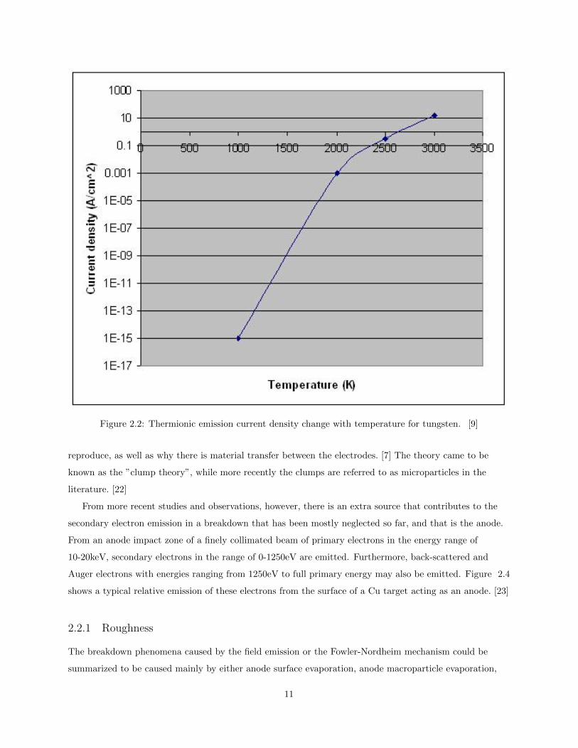
Figure 2.2: Thermionic emission current density change with temperature for tungsten. [9]
reproduce, as well as why there is material transfer between the electrodes. [7] The theory came to be
known as the ”clump theory”, while more recently the clumps are referred to as microparticles in the
literature. [22]
From more recent studies and observations, however, there is an extra source that contributes to the
secondary electron emission in a breakdown that has been mostly neglected so far, and that is the anode.
From an anode impact zone of a finely collimated beam of primary electrons in the energy range of
10-20keV, secondary electrons in the range of 0-1250eV are emitted. Furthermore, back-scattered and
Auger electrons with energies ranging from 1250eV to full primary energy may also be emitted. Figure 2.4
shows a typical relative emission of these electrons from the surface of a Cu target acting as an anode. [23]
2.2.1 Roughness
The breakdown phenomena caused by the field emission or the Fowler-Nordheim mechanism could be
summarized to be caused mainly by either anode surface evaporation, anode macroparticle evaporation,
11
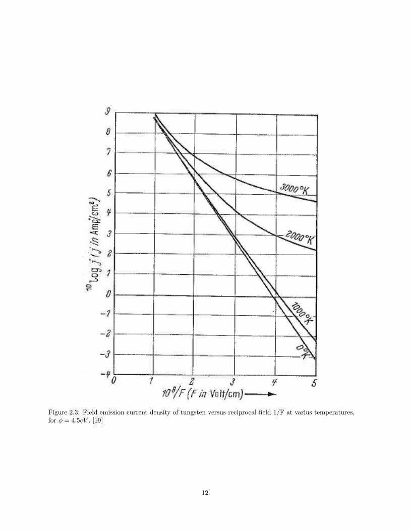
Figure 2.3: Field emission current density of tungsten versus reciprocal field 1/F at varius temperatures,for φ = 4.5eV . [19]
12

Figure 2.4: A typical secondary electron spectra obtained from the impact of a 20kV electron beam on aCu target under low-field conditions. [23]
cathode protrusion evaporation or explosive evaporation of cathode protrusion because of instability.
It has long been speculated and shown, based on whisker field emission models, that the breakdown
holdoff threshold increases as the surface is more refined, and hence there are less sites or sharp tips with
electric fields much higher at them than the average field at the surface of the electrode to initiate field
emission [22]. Recent experimental results however, have indicated that a 50µm sandblast copper surface
treatment (equivalent to grit size of ≈ 300) has decreased the secondary emission in RF systems leading to
multipactoring [13].
2.2.2 Effect of UV radiation on breakdown
As before the breakdown, there is some thermionic or photoelectric emission taking place from the surface
of the cathode that initiates the breakdown by heating up and causing evaporation either on the surface of
the cathode or the anode, it is expected that Ultra Violet radiation should contribute to the photoelectric
emission of electrons from the surface of the cathode. The shortest wavelength light available without the
need to resort to MgF or other especial transparent containters, that can pass through quartz, is 253.7nm
Ultra Violet, used in industry for mostly germicidal purposes. For this reason, a 253.7nm source was
chosen for the UV experiments. The photon energy needed to knock one electron off of a surface of a
material can be calculated by
13

E = hν =hc
λ(2.10)
As the copper work function is equal to 4.7eV, the highest wavelength needed for copper electronic effect
can be calculated to be 264nm. As 253.7nm is not much shorter than 264nm, the photoelectric emission of
the copper was not expected to be significant. Aluminum, on the other hand, has a work function of
4.08eV, and hence is capable of photoelectric emission for any wavelength of radiation shorter than 304nm.
Hence, aluminum was chosen as the material of choice for the cathode during the UV experiments.
2.3 Multipactor phenomena
The vacuum surfaces at 10−7 − 10−6 torr pressures are still covered with multilayers of gas. When RF
voltage is applied to the electrodes in such a vacuum at very low pressure, the so-called multipactor effect
can occur if appropriate boundary conditions (geometry, RF frequency and voltage) are given. The
multipactor starts with single free electrons, which may be present between two electrodes in a
high-frequency electric field. In this field the electrons are accelerated towards one of the electrodes, and
may emit one or more secondary electrons if the impact energy is in the appropriate range. If the polarity
of the electric field reverses at this time, these secondary electrons will be accelerated to the other
electrode, where the same process can take place again. If the amplitude of the electric field, the frequency
and the electrode distance are properly chosen, and the secondary electron emission coefficient for the
energy of impact is higher than unity, the number of electrons will further increase and the multipactor is
established. [10]
14

CHAPTER 3
SIMULATIONS
3.1 Characteristics of the transmission line in the Breakdown Tester atOak Ridge National Laboratory
A model was developed using MATLAB to calculate the reflection coefficient of the breakdown tester
antenna, as well as the voltage and current at each point of the antenna, and compare them to the
measured values from the Breakdown Tester experiment at ORNL.
The characteristic impedance of a transmission line is [6]:
Z0 = sqrt((R+ j × ω × L)/(G+ j × ω × C)) (3.1)
The reflection coefficient is:
ρ = (ZL − Z0)/(ZL + Z0) (3.2)
The voltage along the line is given by:
V (z) = Vicosh(γz)− IiZ0sinh(γz) (3.3)
where i denotes input end and L the load end of quantities. γ is the propagation constant given by
γ = α+ jβ = sqrt((R+ jωL)(G+ jωC)) (3.4)
The code for this model written for MATLAB can be found in Appendix A. The results obtained by
the MATLAB program are shown in figure 3.1.
As can be seen from figure 3.1, the calculated and measured reflection coefficients and the voltage
match perfectly, showing the exact frequency where the best tuning occurs.
15

Figure 3.1: Comparison between the calculated and the measured reflection coefficients of the ORNLBreakdown Tester and the voltage at every point in the antenna.
3.2 Single electron trajectory with RF voltage applied
Multipactoring is a phenomenon that occurs when the RF frequency and electric field at a certain point of
a transmission line are such that electrons emitted from either inner or outer conductor of the line travel to
the opposite conductor in half of the period of the wave. If the surfaces allow for secondary electron
emission, these electrons then multiply and continue traveling between the electrodes while the power is
applied. This can lead to electrical breakdown and arcing in the transmission line, causing possible
damage. To study this phenomenon, a model was developed to show the motion of a single electron in the
gap between the electrodes at the tip of the 1/4-wavelength transmission line which is the Breakdown
Tester setup at ORNL, based on basic equations of motion and Lorenz law. Figure 3.2 shows the position
of an single electron relative to the electrodes:
The Lorentz force equation is
~F = q × ( ~E + ~ν × ~B) (3.5)
16

Figure 3.2: Schematic representation of a single electron located between the two electrodes at the ORNLBreakdown Tester.
Since the electric field will solely be applied in the y-direction, and the magnetic field will solely be
applied in the x-direction, and since the electric field can only apply force in the same direction, and the
magnetic field can apply force using the right-hand-rule only in the direction of velocity crossed with the
magnetic field, assuming an initial velocity of the electron only in y-direction we get electron motion in y
and z directions only. Using basic Newtonian equations of motion, we know that
y = 1/2ay × t2 + ν0y × t+ y0 (3.6)
which applies equally to the z-direction. Using these equations and Newton’s second law, we know
m× a = q × ( ~E + ~ν × ~B) (3.7)
⇒ ay = q/m× (Ey + νz ×Bx) (3.8)
⇒ az = −q/m× (νy ×Bx) (3.9)
Also, the velocities are calculated according to
νy = ay × t+ ν0y (3.10)
and
νz = az × t+ ν0z (3.11)
17

For the following figures, the model was applied for 0.5ns, and the electron was assumed to be at x=0(at
the center of electrodes) and y=-0.5mm(at the lower edge, near the grounded electrode). The initial energy
of electron, corresponding to it moving only in the y direction, was assumed to be ≈ 1eV , and hence
E = 1/2×m× ν2
ν0y =√
2× E/m ≈ 593000m/s
The voltage amplitude was assumed to be 200V. Since this model is for RF power, that means the electric
field at each instant would be different, and would be equal to the alternating voltage divided by the gap
between the electrodes. The alternating voltage at the electrodes was calculated at each instant by using
V = V0 × cos(2× π × f × t), where f was the radiofrequency in Hz, and V0 the initial voltage amplitude.
The magnetic field was assumed to be Bx = 133G.
Figure 3.3: Path of an electron in the y-direction with both magnetic and RF electric fields applied;Vamplitude = 200V , Bx = 0.0133T , ν0y = 593000m/s(≈ 2eV ).
Figures 3.3, 3.4, and 3.5 show the path of the electron in the presence of an electric field (y direction)
and a magnetic field perpendicular to the electric field (x direction). The strength of the fields as well as
the electron initial position and velocity can be varied. Hence, figure 3.3 shows the trajectory of the
electron in the same direction as the electric field, with the magnetic field applied perpendicular to it.
Figure 3.4, on the other hand, shows the trajectory of an electron in the z-direction, with the electric field
in the y-direction and the magnetic field in the x-direction. It can be seen that since the direction of the
18

Figure 3.4: Path of an electron in the z-direction with both magnetic and RF electric fields applied;Vamplitude = 200V , Bx = 0.0133T , ν0y = 593000m/s(≈ 2eV ).
electron’s motion is perpendicular to both the fields, the electric field has no effect, but the magnetic
causes the periodic motion in the z-direction. The lack of electric field’s influence in the z-direction
explains why the trajectory in figure 6 is smoother than that in figure 3.3. Figure 3.5 simply shows both
these motions, so the trajectory of an electron can be traced in the plane perpendicular to the magnetic
field, with the electric field applied in the y-direction. It gives a visual map of how a single electron might
move in the plane parallel and in between the two electrodes in the ORNL Breakdown Tester setup.
Since the gap between the electrodes was assumed to be 1mm, that limits the y-direction motion of the
electron to +0.5mm and -0.5mm in the assumed axis. From the graphs, we can see this means that with
the given conditions, the electron would hit one of the electrodes after 0.23ns. For the z-direction,
assuming a diameter of 3cm before the electron would reach a surface, this would happen after 1.15ns,
according to the model with the given conditions. Clearly, the electron would hit one the electrodes, in less
than a nanosecond, before it had a chance to reach any surface perpendicular to the y-direction. The
figures show the exact path of this solitary electron without taking the boundaries into account.
19

Figure 3.5: Path of an electron in the z and y-direction (plane perpendicular to the magnetic fielddirection) with both magnetic and RF electric fields applied; Vamplitude = 200V , Bx = 0.0133T ,ν0y = 593000m/s(≈ 2eV ).
20

CHAPTER 4
DESCRIPTION OF EXPERIMENTS AND RESULTS
The experiments referred to in this work were carried out in two locations, at the SPARCS setup at the
Center for Plasma Material Interactions at the University of Illinois at Urbana-Champaign, and at the
Breakdown Tester setup at the Fusion Energy Division of Oak Ridge National Laboratory.
4.1 University of Illinois
4.1.1 SPARCS setup
The SPARCS experiment setup at the Center for Plasma Material Interactions at Uiversity of Illinois took
place in a cylindrical steel vacuum chamber, 36” in diameter and 10” in height. The chamber was
originally donated by Intel and was part of a Plasma Etcher Model 425. The chamber features many
windows and connection ports. The chamber lid is lifted with an automatic arm, and the connection
features an oversized elastomer o-ring. This gives an access to the chamber with the 36” diameter, which
allows ample space to work and modify the chamber, however, the o-ring limits the ultimate low pressure
the chamber can reach.
The chamber used two vacuum pumps to evacuate. It was initially pumped down by a belt-driven Duo
Seal Model 1397 roughing pump to reach mTorr range. The pump was connected to a bakeable zeolite oil
trap in order to eliminate oil particles polluting the chamber. Afterwards, the valve between the roughing
pump and the chamber was closed and it was used to back up the turbomolecular pump capable of
pumping down the chamber ultimately to 10−8 Torrs. The turbomolecular pump used for the chamber was
changed twice during the experiments. Initially a BOC Edwards turbo molecular pump model
EXT250/100CF was used, which was later switched to a Varian V301 Navigator pump, and later to a
Varian V301 turbo molecular 300 l/s pump. Most of the experiments were performed using the latter
pump. The chamber pressure on average was between 10−7 − 10−6 Torrs, however, the chamber was
capable of reaching an ultimate pressure of mid 10−8 Torrs after repetitive bakeouts and prolonged
pumpdowns, despite having a large o-ring between the lid and the chamber.
There were four 1.2 kW internal halogen lamps installed in the chamber to allow bakeout. The
chamber was pumped down to a maximum of 2.80 · 10−6s, at which point it was originally baked out once
21

and allowed to cool down before performing the experiments, but later on started to do it two to six times:
bakeout once (range: 160◦C-143.3◦C) with electrodes far away, let it cool off
(range:46.1◦C)-24.9◦C)-measured without equivalent load) and pump down again for at least an hour, then
bring the electrodes closer (about 20− 25µm) and bake out again (range:164.5◦C-112.7◦C). The result was
a maximum of low 10−7 Torr pressures. Starting on April 30th, 2008, the chamber was flushed with argon
before turning on the turbopump, in order to get rid of some of the water vapor. The first time, the
chamber was brought up to about 350 Torr (6 Torr on convectron reading) using high-purity Argon (using
the convectron calibrated for N2), and then pumped down.
Pressures above 0.5 mTorr were measured using a Granville-Phillips 275 mini-convectron gauge. The
convectron gauge was calibrated for N2, though not very accurately. However, it was mainly used to
indicate the time to start the turbopump. Pressures below 5 · 10−5 Torr were measured using a glass
Alpert-Ballard ionization gauge, controlled by a Granville-Phillips 341017 Vacuum Gauge Controller
interfaced with a PC computer running Labview 6.1. This gauge provided reproducible and consistent
pressure readings, though it was not very accurately calibrated either. The ionization gauge was at the end
of its lifetime, and for a couple times got stuck at a certain pressure after breakdowns. Turning it down
and back on after a bit would cause it to resume normal behavior.
The Labview program was also connected to three Mass Frow Controllers capable of delivering gas in
controlled conditions. The chamber also featured an SRS Residual Gas Analyser to detect the gases
present in the chamber and their proportions. The electrode temperature was monitored with a
thermocouple placed near the electrode gap in the chamber. Initially the thermocouple was not attached
to a dummy load, hence the temperature readings were corrected to indicate the temperature of the anode
electrode. Later on, a dummy electrode of the same type as the anode was attached to the thermocouple in
order to have more accurate readings.
For the breakdown experiments, a General Atomics (previously Maxwell Labs) Capacitor Charging
Switching (CCS) model CCS-08-050-P-1-0000-C DC power supply was used. This positive polarity power
supply works by charging a capacitor, and can provide a maximum of 50 kV rated at 8 kW. It required a
capacitive load present at all times to work properly, hence a capacitor capable of charging to a maximum
of 15 kV was used. The power supply also required protection for polarity inversion for use in breakdown
experiments. For the stable operation of the supply, an inversion circuit protection was provided by
twenty-two RURG80100 (80 A, 1000 V) ultrafast diodes in series, allowing a maximum current of 80 A to
be delivered during breakdown. [3] The power supply was connected to the cathode, and it was possible to
deliver 0 to -15 kV of DC voltage to the cathode. The anode was grounded. Figure 4.1 shows the power
supply on the left and the capacitor it charged, which in turn was connected to the cathode, on the right.
The power was delivered to a flat-surface cathode of 1.5” diameter, facing a semi-spherical anode of
3/4” diameter. The distance between the electrodes was controlled by a Huntington Labs Micrometer
linear motion feedthrough with an accuracy of ±1µm in the horizontal direction. The gap between the
22

Figure 4.1: The 50 kV DC power supply on the left and the max. 15 kV charging capacitor on the right.
Figure 4.2: Schematic of the inversion circuit to protect the power supply by allowing a maximum currentof 80 A during breakdown. It included twenty-two RURG80100 (80 A, 1000 V) ultrafast diodes in series.
electrodes was adjusted by nearing the electrodes until they touched, using a multimeter to check for
continuity, and afterwards distancing the electrotodes to the desired distance. 150µm± 1µm was the main
distance at which the electrodes were set at the beginning of each experiment. However, since the
temperatures were often above the room temperature due to starting the experiments right after bakeouts
to minimize gas coverage of the electrode surfaces, they continued to drop and the electrode gap continued
to change during the experiment due to contraction. Hence, the gap distance and temperature were also
recorded at the end of each experiment, and the gap distance during the breakdown was calculated
assuming a linear contraction rate based on temperature.
A schematic view of the experiment can be seen in figure 4.3, and a diagram of it can be viewed in
figure 4.4.
23
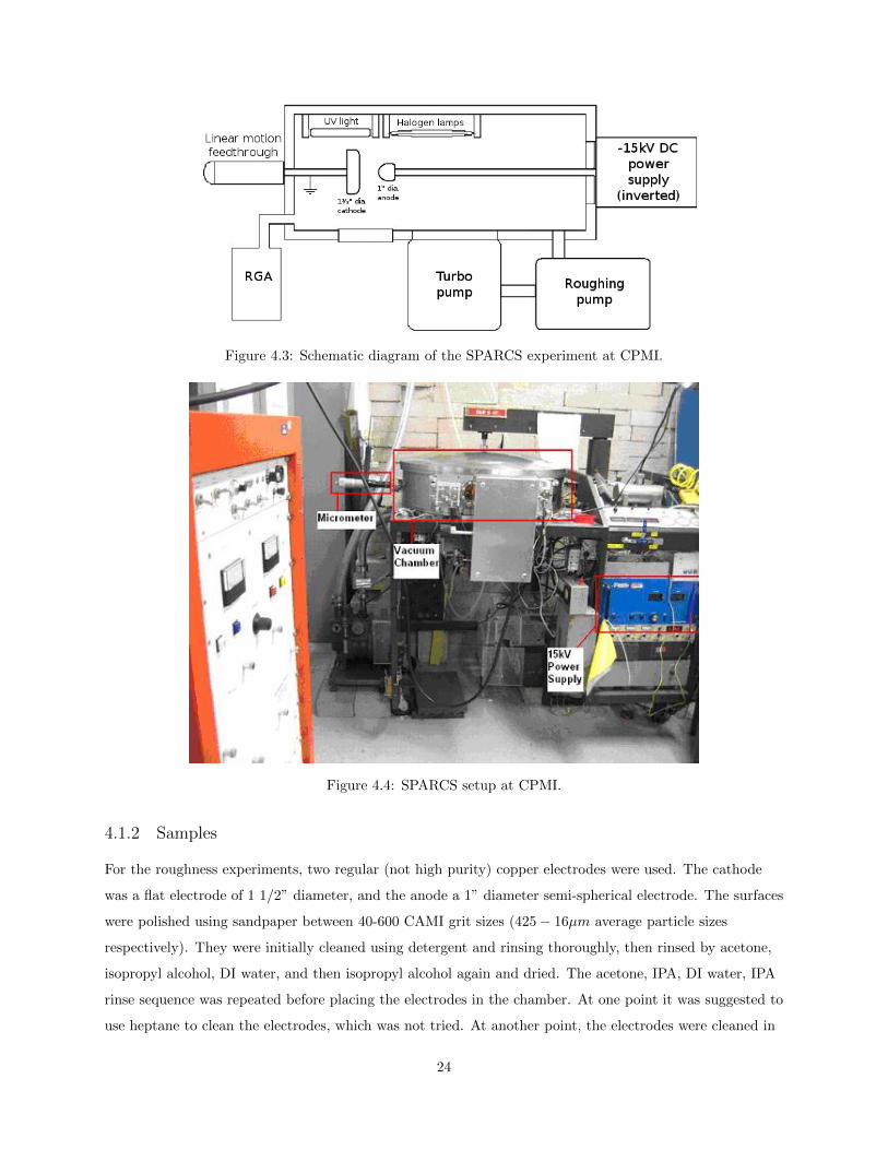
Figure 4.3: Schematic diagram of the SPARCS experiment at CPMI.
Figure 4.4: SPARCS setup at CPMI.
4.1.2 Samples
For the roughness experiments, two regular (not high purity) copper electrodes were used. The cathode
was a flat electrode of 1 1/2” diameter, and the anode a 1” diameter semi-spherical electrode. The surfaces
were polished using sandpaper between 40-600 CAMI grit sizes (425− 16µm average particle sizes
respectively). They were initially cleaned using detergent and rinsing thoroughly, then rinsed by acetone,
isopropyl alcohol, DI water, and then isopropyl alcohol again and dried. The acetone, IPA, DI water, IPA
rinse sequence was repeated before placing the electrodes in the chamber. At one point it was suggested to
use heptane to clean the electrodes, which was not tried. At another point, the electrodes were cleaned in
24

acetone by ultrasonic cleaning, but this was not tried for all the electrodes.
The surface roughness of the electrodes was measured with a Sloan Dektak profilometer, and for lower
roughnesses (higher than 120 CAMI grit size), Atomic Force Microscopy was used as well. Figure 4.5
shows a pair of polished copper electrodes.
Figure 4.5: A cathode with a 40 grit sandpaper finish on the left next to an electropolished anode.
Three roughness measurements were made with each instrument, the arithmetic roughness, the
root-mean-square roughness, and then 10-point height average. These roughnesses are defined as
follows [29] and [14]:
Ra - Arithmetic average roughness or mean roughness: It is the universally recognized, and most used
international parameter of roughness. It is the arithmetic average deviation from the mean line. It is
calculated using
Ra =1
n
n∑j=1
|Zj | (4.1)
Rq - Root-mean-square roughness: It determines the root-mean-square value of roughness
corresponding to Ra, and can be calculated using
Rq =
√∑(Zi)2
n(4.2)
Rz - 10-point average roughness: It is the average height difference between the five highest peaks and
the five lowest valleys in accordance with DIN 4768/1 specification published by the Deutsche Institut fuer
25

Normung c.v.
Figure 4.6: Cathodes with various surface finishes. The grit size of the sandpaper last used is shown nextto each electrode. The concentric circles that can be seen on electrodes with sandpaper finish is a result ofpreparation method of sanding with the use of drill press, which results in surface waviness, which needs tobe taken into account when calculating surface roughness.
Figure 4.7: Roughness values vs average particle diameter of sandpaper.
26

Figure 4.8: Arithmetic and RMS roughness values vs average particle diameter of sandpaper.
Figure 4.9: Electrode profile taken via DEKTAK profilometer.
Figure 4.9 shows the profile of the electrode taken with the profilometer. As can be seen, the surface
has a natural curvature due to the polishing procedure of mounting the electrode on a drill press, and
pressing the sandpaper to it while it is rotating. Even though the angular velocity if the same everywhere
on the electrode, because of a higher tangential velocity towards the edges of the electrode compared to the
center, the electrode is unevenly etched, with the edges polished more than the center, which causes the
27

curvature that can be seen in the image. In profilometry practices, this curvature is referred to as waviness,
and it can affect the roughness measurements. In order to prevent this from happening, separating the
roughness and waviness is achieved by using filter cut-offs [5]. Figure 4.10 shows the different roughness
values measured via profilometry vs different cutoff filters, ranging from 10µm to 600µm, across four
parallel lines of 4cm length across an electrode polished with a 40 CAMI grit sandpaper. It can be observed
that the graphs seem like two separate linear graphs with different slopes, joined in a curvature around
100µm. The left linear slope shows how as the cutoff filter length increases, more of the roughness features
are being taken into account, while the waviness does not come into play until about 100µm, where the
next linear slope starts. The new slope shows that all roughness features are now being taken into account,
however, as the cutoff filter length increases even further, the waviness comes to be taken into account
further as well. In order to take most of the roughness features into account, while filtering the waviness of
the surface out, the cutoff filter at the intersection of the two linear slopes was chosen; namely, 100µm.
Figure 4.10: Various measured profilometry roughnesses for diffferent cutoff filters used.
Various roughness measurement comparisons can be seen in figure 4.7. For better comparison,
figure 4.8 shows only the arithmetic and root-mean squared roughness measurements. It can be observed,
that for similar sandpaper grit size, different measured roughnesses were obtained, pointing to the
roughness not being only dependent on the sandpaper grit size used; hence, roughness measurements were
done for each electrode used. Also observe, that the AFM roughness measurement is limited to smaller
roughnesses (higher grit sizes) only, typically higher than 120 CAMI grit size (less than 125µm average
28

Figure 4.11: Roughness measurements vs different roughness filter cutoffs for four parallel lines across thesurface of a 40-grit polished electrode.
particle size of the sandpaper).
Figure 4.12: Roughness measurements showing arithmetic roughness, root-mean-squared roughness, and10-point height average roughness taken via profilometry and atomic force microscopy.
For the UV experiments, the same procedure was applied, except instead of copper, aluminum
29

Figure 4.13: Roughness measurements showing arithmetic roughness, root-mean-squared roughness, and5-point average roughness taken via profilometry and atomic force microscopy.
electrodes with a 2” diameter were used as cathodes, and electropolished semi-spherical electrodes were
used as anodes. The electropolishing was done using a 3-1 ratio of phosphoric acid (H3PO4) and DI water
solution as an electrolyte, and a stainless steel shimstock as a grounded cathode. The for electropolishing
can be viewed in figure 4.14.
Figure 4.14: Circuit used for electropolishing the copper electrodes.
The electrode was electropolished for about 20 minutes each time. A sample of the evolution of the
electropolishing voltage and current can be seen in table 4.1.
30

Table 4.1: Sample of current and voltage change while electropolishing.
Time (min) Voltage (V) Current (A)1 1.363 0.483 1.500 0.405 1.500 0.3210 1.501 0.3215 1.501 0.3220 1.501 0.3225 1.501 0.32
4.1.3 Experiments and results
4.1.3.1 Copper anode and cathode both with equal roughness experiments
For the roughness experiments, the chamber was pumped down by the roughing pump and then by the
turbomolecular pump. When the pressure was in 10−7 − 10−6torr range, the halogen lamps set up in the
chamber were turned on and the chamber was heated up to 120◦C − 150◦C. At this point the chamber
would be baked out, which would cause gas molecules and atoms to be desorbed from the surfaces, causing
the pressures to rise up to 10−6torr, after which it would start to go back down as the turbomolecular
pump kept working. The chamber was consequently put to a vacuum of 10−8 − 10−7torr. As after cooling
down, it takes a short while for the gas to be readsorbed again in the walls of the chamber, the chamber
was baked out once more right before running an experiment, and this time the experiment was run when
the temperature was still in the 60− 80◦C range before the chamber cooled down again. In some of the
roughness experiments, constant roughness anode experiments and the UV experiments, after pumping
down the chamber with the roughing pump, the chamber was flushed with high purity Ar before being
pumped down to a vacuum of 10−8 − 10−6torr.
Afterwards, as can be seen in figure 4.3, the electrodes were brought together using the linear motion
feedthrough. Both electrodes were temporarily grounded, and at the same time short circuited through a
multimeter, set to detect contact. The electrodes were visually inspected through a chamber window until
they were quite close, at which point they were gently and slowly brought together further until a contact
was detected. The location was recorded and the electrodes were taken apart by 150µm (and in a few cases
with hard-to-achieve breakdown fields, to 100µm). As mentioned before, the precision of the linear motion
feedthrough is within 2µm.
The chamber was baked out 2-3 times before running the experiments, in order for the the gas
molecules to desorb from the surfaces. These experiments were run starting with regular air in the
chamber, which was pumped down to 10−7 − 10−6torr. Regular air contains an average of 1% water vapor
which in comparison with other gases is particularly apt to adhere to the surfaces of solids by van der
Waals forces (physisorption with binding energies of less than 40 kJ/mol or chemisorption with binding
31

Table 4.2: Monolayer formation time calculated for baked out vaccuum surfaces around the range of30− 65◦C
Pressure Monolayer formation time at 300 K Monolayer formation time at 340 K(torr) Air (s) H2 (s) H2O (s) Ar (s) Air (s) H2 (s) H2O (s) Ar (s)760 3.3 · 10−9 8.7 · 10−10 2.6 · 10−9 3.9 · 10−9 3.5 · 10−9 9.2 · 10−10 2.8 · 10−9 4.1 · 10−9
1 2.5 · 10−6 6.6 · 10−7 2.0 · 10−6 3.0 · 10−5 2.7 · 10−6 7.0 · 10−7 2.1 · 10−6 3.1 · 10−5
10−3 2.5 · 10−3 6.6 · 10−4 2.0 · 10−3 3.0 · 10−2 2.7 · 10−3 7.0 · 10−4 2.1 · 10−3 3.1 · 10−2
10−6 2.5 0.66 2.0 30 2.7 0.70 2.1 3110−10 2.5 · 104 6.6 · 103 2.0 · 104 3.0 · 105 2.7 · 104 7.0 · 103 2.1 · 104 3.1 · 105
energies of 80 kJ/mol and 800 kJ/mol) [18]. This process is called adsorption, and though physisorbed
gases quickly desorb in room temperature, the chemisorbed gases cause the inner surfaces of a vacuum
chamber to be normally covered with monolayers to multilayers of their atoms or molecules. This can
interfere with the breakdown experiments as it increases the number of potential mechanisms that can
contribute to breakdown. Therefore, the chamber was baked out using four halogen lamps before each
experiment to cause the water vapor and other gas molecules and atoms to desorb from the electrode
surfaces. The halogen lamps were then turned off and the chamber pumped down again to reach
10−8 − 10−7torr pressure. The time required before a clean, desorbed surface gets covered with a
monolayer of gas again was given by equation 2.5, which can be used to calculate the monolayer formation
times for the gases used in our experiments. So for example for air (Mr ≈ 29) at 300K, we get:
tmono[s] =3.4 · 10−4
p[Pa](4.3)
At 10−6torr, it takes ≈ 2.0− 2.7s for the surfaces to be covered by a monolayer of air (1% water vapor)
and ≈ 30s for a monolayer of argon, while at 10−8torr it takes ≈ 3.3− 4.5min for air and ≈ 50min for
argon. In order to minimize gas coverage of the electrode surfaces during the experiment, the chamber was
baked out when the pressure was in 10−7-high 10−8torr range. As the chamber was heated up, the
pressure rose to low 10−6 − 10−7torr range. Just before starting the experiments, the halogen lamps were
turned off so as not to interfere with the experiments; however, as the chamber gradually cooled down
during the experiment, the distance between the electrodes, which was carefully measured with the
micrometer by slowly and lightly touching the surfaces of the electrodes at the beginning of the experiment
and then bringing them to a certain distance, kept changing due to thermal contraction. The distance
between the electrodes was measured at the end of the experiment, when the chamber had cooled down
again, and assuming a linear contraction of the electrodes with declining temperature, the distance at each
point of the experiment could be calculated based on the temperature assuming a linear thermal
contraction to correct for the electric field at the time of the breakdown.
32

dbreakdown − dinitialTbreakdown − Tinitial
=dfinal − dinitialTfinal − Tinitial
(4.4)
It should be noted that in these experiments, the thermocouple was not connected to an equivalent
load. In order to have the exact temperature at the electrode surfaces measured by the floating
thermocouple, the thermocouple was later calibrated by attaching a dummy load equivalent to the anode
(a 1” semi-spherical hollow copper piece). Two bakeouts were performed, one with the thermocouple
attached to the equivalent load and one without, starting at room temperature equilibrium and then
heating up the chamber for 11 minutes and then turning off the halogen lamps and letting it cool down.
The temperature pace in both cases can be seen and compared in figure 4.15. It is interesting to note the
hysteresis which makes the temperature rising pace different from the declining pace. It must be noted
that the pressures in both measurements were comparable, starting at 3.90 · 10−7torr in one and
3.00 · 10−7torr in the other, and reaching 4.70 · 10−6torr and 3.90 · 10−6torr at their peak.
Figure 4.15: Thermocouple temperature reading during and after bakeout with and without 1” hollowcopper semi-spherical dummy load
.
Since the experiments were performed immediately after the halogen lamps were turned off, the
temperature calibration was done using the declining portion of the temperature vs time graph
(figure 4.15).
Baking out and starting the experiment before the surfaces cooled down had the positive effect of
keeping the surfaces gas-free for longer and partially eliminating gas desorption as a control factor
contributing to the mechanism of breakdown. However, it had one disadvantage. As can be seen in
figure 4.17, breakdowns at higher voltages happened at lower temperatures, while breakdowns at lower
33

Figure 4.16: Thermocouple temperature with mass vs thermocouple temperature without mass
voltages happened at higher temperatures. While this may lead one to conclude the breakdown
dependency on surface temperature, with higher thermionic emission at higher temperatures causing lower
breakdown threshold, this could not be concluded from these experiments, as both temperature and
voltage were functions of time: As the time went on during the experiment, the temperature kept dropping,
while the voltage kept being raised (the voltage was varied only by increasing during all experiments to
avoid hysteresis effects). Therefore, while breakdown electric field may indeed be dependent on thermionic
emission and hence the temperature of the surface, that cannot be concluded from these experiments.
Figure 4.18 shows the surface topography of a copper cathode with a 320 sandpaper finish. In these
experiments, it was hoped to establish whether the fineness of such surface features cause any substantial
difference in the electric field required for a breakdown.
Figure 4.19 shows an SEM image of the effect of breakdown on the surface of an electrode (not the
same spot). As can be seen, after the breakdown the electrode looks like a sea with waves that was frozen
in an instant.
Table 4.3 shows the summary of the results that were obtained from the roughness experiments, which
were run to determine their effect on the breakdown threshold.
Figure 4.20 shows the virgin electrode breakdown field for copper electrodes in all the experiments
where the anode and the cathode were of equal roughness, regardless of whether the chamber was flushed
with high purity argon pre-bakeout or not. The vertical error bars show the standard error. From this
graph, no clear pattern can be established between the sandpaper surface finish roughness and the
34

Table 4.3: Results of the copper electrode roughness experiments with both anode and cathode sandpaperfinished with the same grit. Results include chamber pumped down from laboratory air as well as results ofthose with chamber flushed with high purity argon. The temperatures are calibrated for thermoucoupleattached to anode-sized electrode.
Gas Electrode Grit Ra(nm) Rq(nm) Tb(◦C) P (torr) db(µm) Iavg,b(µA) Vb(kV ) Eb(
MVm )
Air
16 40 13253 16864 39.0 5.00 · 10−7 239 9.686 12.030 50.417 220 4649 6080 36.9 5.20 · 10−8 200 0.222 8.080 40.318 320 1917 2478 55.0 1.00 · 10−6 157 1.345 4.560 29.019 500 1717 2221 55.1 1.40 · 10−7 167 2.587 5.485 32.720 120 11475 14559 62.4 3.90 · 10−7 158 0 2.992 19.021 400 1537 2000 49.6 5.50 · 10−8 165 0.001 3.997 24.324 600 1571 2029 45.2 5.50 · 10−8 204 4.79 8.690 42.725 80 18197 23675 55.1 1.70 · 10−7 191 0.286 4.013 21.026 50 22978 28608 51.7 1.20 · 10−7 150 0.064 4.512 30.127 60 13490 16982 56.9 5.70 · 10−7 113 2.266 5.001 44.128 100 9269 11873 52.9 1.80 · 10−7 209 0.067 7.590 36.429 50 10418 13225 56.8 7.70 · 10−8 179 1.214 3.428 19.130 500 1039 1368 52.0 1.30 · 10−7 194 2.323 4.898 25.231 100 8803 11559 56.2 1.00 · 10−7 164 24.652 5.644 34.432 80 9843 12550 62.4 5.00 · 10−7 159 0.001 2.784 17.633 60 8524 10754 57.1 1.00 · 10−7 174 0.008 3.902 22.535 80 6523 8233 54.2 5.40 · 10−8 160 0.02 3.576 22.436 600 1390 1903 31.0 8.50 · 10−8 169 0.004 3.070 18.2
34 60 15508 20201 37.3 7.20 · 10−8 202 0.028 6.405 31.7
Arg
on
37 50 15712 20300 34.4 7.20 · 10−8 184 53.71 7.500 41.038 100 6613 8611 35.6 6.20 · 10−8 179 1.735 8.410 47.139 80 7620 9596 37.8 5.10 · 10−8 211 13.051 7.170 34.043 40 11614 14469 36.5 9.20 · 10−8 184 0.446 6.013 32.844 320 1805 2349 35.7 6.50 · 10−8 226 2.745 11.00 48.745 400 2173 2831 38.5 1.60 · 10−7 218 1.742 6.447 29.646 120 3455 4469 35.5 5.00 · 10−8 201 27.557 7.020 35.0
35

Figure 4.17: Electric field at breakdown vs electrode temperature for air and argon vaccuums.
Figure 4.18: Surface features plot using Digital Instruments Dimension 3100 AFM across a 5× 5µmsurface of a copper electrode with a 320 grit sandpaper finish (Ra = 1917nm). The vertical scale is 1.5µmdiv .
breakdown electric field. For comparison, in an experiment with both electrodes having an electropolished
surface finish, where the chamber was let to cool down after the last bakeout before starting the
experiment, the virgin electrode breakdown field was 47.0MV/m, possibly caused by gas molecule
36

Figure 4.19: SEM images of typical electron surface before and after a breakdown.
desorption from the surface of the electrodes as it happened right in the beginning of the experiment
without much current. The second breakdown in the electropolished case happened at 91.4MV/m.
Figure 4.20: Breakdown electric field vs average roughness for copper electrodes where both anode andcathode were of equal roughness with sandpaper finish in each experiment, regardless of the gas in thechamber.
In figure 4.21 the same cases can be seen, except the cases where the chamber was pumped down
directly from atmospheric pressure have been separated from those where the chamber was flushed with
high purity argon before the bakeout. Again, there is no clear pattern showing dependence on surface
37

roughness. However, the average virgin electrode breakdown field is higher by 7.8MV/m in cases where the
chamber was flushed with argon. The average breakdown electric field was 29.4± 10.1MV/m for the
chamber filled with regular air, and 36.9± 7.2MV/m for experiments flushed with high purity argon. Both
electrodes were made of copper in all cases, and the anode and cathode had equal grit sandpaper finish.
The horizontal standard error bars have also been included.
Figure 4.21: Breakdown electric field vs average roughness for copper electrodes where both anode andcathode were of equal roughness. The experiments in which the vaccuum was pumped down fromlaboratory air have been separated from those where the chamber was flushed with high purity argonbefore bakeout.
These experiments were carried out before the chamber was allowed to cool down, starting the
experiment anywhere between 34− 73◦C, in order to minimize surface readsorption of gas molecules and
be able to rule out desorption initiated breakdown as a mechanism in these experiments. As a result, a
temperature dependence seems to emerge (as seen in 4.17), which is a result of temperature decreasing
and voltage increasing with time, and is inconclusive in establishing a dependence between breakdown
voltage and temperature, though the figure may suggest otherwise. Figure 4.17 shows the breakdown field
vs average roughness for experiments performed with air in the chamber separated based on different
temperature ranges. The argon cases are not displayed as all of them happened in the range of 30− 40◦C,
and the graph would be exacly the same as 4.21.
Figure 4.23 shows the current averaged over 1− 3min vs average roughness. One data point was
eliminated based on Chauvenet’s criterion. There does not seems to be any clear pattern of dependence
between current emitted during breakdown and roughness nor temperature.
38

Figure 4.22: Breakdown electric field vs average roughness for experiments performed in air with copperanode and cathode of equal roughness in different temperature ranges.
Figure 4.23: Breakdown current averaged over 1− 3min vs average roughness for experiments performed inair with copper anode and cathode of equal roughness in different temperature ranges.
Figure 4.24 shows the breakdown electric field vs roughness again, but this time with data broken down
based on pressure ranges where there breakdown happened.
To make sure that the roughness around the breakdown was not significantly different from the
39

Figure 4.24: Breakdown electric field vs average roughness for experiments performed in air with copperanode and cathode of equal roughness in different pressure ranges.
roughness everywhere else on the electrode, which might have altered the results, the roughness around the
breakdown for some of the cathodes was measured and compared to the general roughness of the cathode.
The roughness around breakdown was measured along 4 lines intersecting at right angles with each other
around the breakdown, each of them 300µm long. The result, as can be seen in figure 4.25 shows a linear
relationship between the two, showing that they are related, and the breakdown threshold would look as
scattered vs the roughness around breakdown as well.
4.1.3.2 Experiments with constant roughness cathode
Four experiments were performed, where electropolished flat copper cathodes were used. The anodes were
semispherical copper electrodes finished with 40, 50, 400 and 600 grit sandpaper, so their average surface
roughnesses ranged between 1826− 21790nm based on roughness averaged over five 3mm lines passing
through the semi-spherical anode’s center in different directions divided into 100µm cutoffs using the
profilometer software to account for the waviness of the anode profile (a semi-sphere of 1” diameter). The
experiments were run after baking out after the chamber was flushed with high purity argon. The results
(figure 4.26), once again, show nearly uniform electric field distibution across different anode roughnesses.
The average electric field is 43.5MV/m, which is 6.6MV/m higher than the average breakdown field for
the experiments where both anode and the cathode had equal roughnesses that were being varied. This
suggests that at least some of the breakdowns are cathode initiated such that using an electropolished
cathode enhances the breakdown threshold. For comparison reasons, in one experiment where both the
40
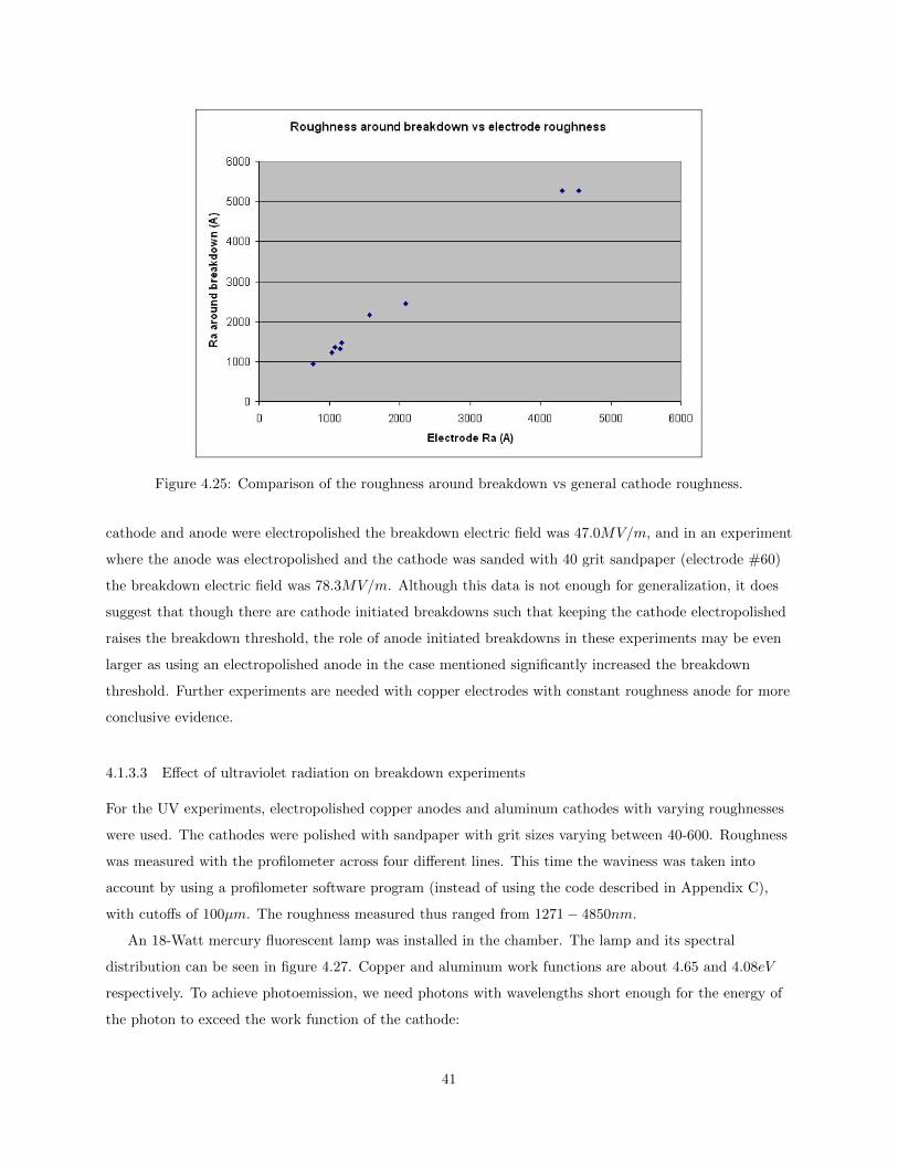
Figure 4.25: Comparison of the roughness around breakdown vs general cathode roughness.
cathode and anode were electropolished the breakdown electric field was 47.0MV/m, and in an experiment
where the anode was electropolished and the cathode was sanded with 40 grit sandpaper (electrode #60)
the breakdown electric field was 78.3MV/m. Although this data is not enough for generalization, it does
suggest that though there are cathode initiated breakdowns such that keeping the cathode electropolished
raises the breakdown threshold, the role of anode initiated breakdowns in these experiments may be even
larger as using an electropolished anode in the case mentioned significantly increased the breakdown
threshold. Further experiments are needed with copper electrodes with constant roughness anode for more
conclusive evidence.
4.1.3.3 Effect of ultraviolet radiation on breakdown experiments
For the UV experiments, electropolished copper anodes and aluminum cathodes with varying roughnesses
were used. The cathodes were polished with sandpaper with grit sizes varying between 40-600. Roughness
was measured with the profilometer across four different lines. This time the waviness was taken into
account by using a profilometer software program (instead of using the code described in Appendix C),
with cutoffs of 100µm. The roughness measured thus ranged from 1271− 4850nm.
An 18-Watt mercury fluorescent lamp was installed in the chamber. The lamp and its spectral
distribution can be seen in figure 4.27. Copper and aluminum work functions are about 4.65 and 4.08eV
respectively. To achieve photoemission, we need photons with wavelengths short enough for the energy of
the photon to exceed the work function of the cathode:
41

Figure 4.26: Breakdown field vs roughness for electropolished copper cathode and varying roughness anode.
hc
λ≥ φ (4.5)
The spectrum of the UV light installed in the chamber dominantly had a wavelength of 254nm, which
means the work function had to be less than or equal to 4.88eV . This wavelength is in the UVC range
(100− 290nm) as well as the Lyman alpha radiation (≈ 122nm), which is what can be expected in
tokamaks and other fusion devices (compare with UVA – 320− 400nm and UVB – 290− 320nm).
Figure 4.27: Emission spectrum of an 18W Philips UV disinfection lamp used for the UV experiments andthe lamp.
Six control experiments were performed without the UV light, in which case the light was covered by
an aluminum foil during the experments. In some, the UV light was turned on while covered during the
experiments to simulate gas desorption as in experiments with the light. In all experiments, the chamber
was flushed with high purity argon before being baked out. In some of these experiments, an attempt was
made to keep the temperature constant by occassionally turning on the halogen lamps and then turning
them off. This caused extra complexities in calculating the distance between the electrodes in cases where
42

the thermocouple was not attached to an equivalent mass equal to the anode, as whether the temperature
was rising or declining at each point took on importance because of hysteresis effects of temperature with
time.
Figure 4.28 summarizes the results of these experiments.
Figure 4.28: Effect of presence of ultraviolet on breakdown electric field. Flat Al cathodes with varyingroughness and electropolished semi-spherical Cu anodes were used. Chamber was flushed with high purityAr before bakeout.
As can be observed, the range for breakdown electric field overlaps in both cases, and there does not
seem to be a very clear dependence on surface macro roughness. However, the average electric field causing
breakdown was 12.3MV/m lower in electrodes exposed to UV than those that were not. The electrodes
that were exposed to UV broke down at an average of 50.2± 17.7MV/m electric field, while the control
cases broke down at 62.5± 11.5MV/m. This can possibly point to contribution of photoemission added to
the effects of field emission, however, since the standard deviation of the data is rather huge, it eclipses the
difference in the averages that was observed, and will need more data points in the future to conclude that
photemission does effectively lower the breakdown threshold.
Figure 4.29 documents the gases present in the chamber before and after the experiment and with and
without the UV lamp on. It shows that though the chamber was flushed with high purity argon before any
bakeouts were done, the contribution was not significant, as water presence (with a significant peak at 18)
is significant in the chamber followed by air and then argon. Also, as can be seen, turning on the UV light
before the experiment increases the gas pressures (confirmed by the ion gauge as well) suggesting
desorption caused by UV. After the experiment, however, the UV being on or off does not change the
pressures significantly, possibly because having been for a prolonged period throughout the experiment, it
has caused the gas to desorb from the surfaces leaving not much else. There are also trace amounts of
43

turbopump oil observable through the graphs.
Figure 4.29: RGA readout showing the pressure of various gases by molecular mass number before andafter experiment with and without the presence of UV light.
4.2 Oak Ridge National Laboratory
4.2.1 Breakdown Tester setup
The breakdown tester is an instrument consisting of an RF signal generator, a trigger signal generator, a
powerful amplifier, 1/4-wavelength transmission line consisting of coaxial cables and matching capacitors
and inductances (47.4MHz, Q 800). Both inner and outer conductor electrode pieces can be removed easily
to test different configurations, materials, or orientation with respect to an external B-field. In this fashion,
the highest voltage possible in the circuit can be achieved at the tip of the electrode, without having too
large of a voltage anywhere else in the circuit to cause a breakdown anywhere but at the tip, however,
multipactor phenomenon can be generated along the transmission line. The high voltage in the gap of
1mm is greater than 30kV, and a magnetic field of 1.2kG can be applied. The UV light source used was a
100W EG & G model 2020C strobe.
The diagnostic devices that were used included two network analyzers for the forward and reflected
power, and the magnitude and phase angle relative to the forward power of the signal at the probe, which
was in turn diagnosed using a probe at the end of the circuit near the high voltage electrode, which picked
up the voltage of the electrode through coupling. An oscilloscope was used to monitor the DC bias caused
by electron current at the center conductor of the transmission line, relative to the trigger signal.
44

Figure 4.30: High Voltage Breakdown Tester schematic at Oak Ridge National Laboratory.
Figure 4.31: Experimental setup of the Breakdown Tester experiment at Oak Ridge National Laboratory.The end of the transmission line leading to the electrodes can be seen, as well as the magnets locatedaround the chamber enclosing the electrodes. The 20 kW transmitter to power the system can be seen inthe background. The silver box behind the blue control box is the matching network.
4.2.2 Experiments and results
4.2.2.1 Breakdown experiments
During Summer of 2006, a camera was setup in front of the view port of the Breakdown Tester system to
correlate the phenomenon happening, especially when viewed slowly, to the pressure and voltage at which
45

the breakdowns were happening. The camera was set up facing the electrodes, while the rest of the view
port was covered with a plastic in order to eliminate external light for two reasons: increase the
detectability of any arcing, and prevent the camera from saturation. The camera signal went through a
time stamper, then a Videocassette Recorder, and eventually to the monitor. The VCR recorded clips of
the breakdowns when they were happening, and was paused for the rest of the time. Afterwards, the movie
clip was transferred to a Mac mini through an analog to digital converting hardware called ProView USB,
and was later imported into iMovie, and individual frames of the breakdowns were extracted. There were
three types of breakdowns: a light glow of the electrode tips, which are hencefore referred to as emission,
and were suspected to be electrons accelerated through material because of the high electric field colliding
with the copper atoms and heating them up, and causing them to emit light. The other kind was a
brighter glow that extended between the electrodes, which are henceforth referred to as arcs. These were
usually with a green glow, suggesting that they were copper plasma. This can be explained by the electric
field being so high that the copper ions accelerated across the electrodes, creating these arcs. This can be
verified noticing that the arcs usually happened at higher powers. The other kind of breakdown happened
at a different section of the transmission line (not at the electrodes). This was a plasma created with every
pulse at higher powers and higher pressures. If the matching and the frequency were appropriate to create
a plasma, this phenomenon occurred at even very low powers when there was a high pressure of gas
present in the vacuum. The color of the plasma of course depended on the type of gas in the tube. The
data collected in this fashion was then organized, and each breakdown description and the frames
correlated with the appropriate pressure, which was obtained from the ion gauge, or some cases convectron
gauge readings, and the appropriate power, which was calculated from the network analyzer readings.
Figure 4.32: Phenomenon occuring with hydrogen gas present in the chamber: A) Emission withP = 1.75× 10⁻⁷torr; B) Arc with P = 1.75× 10⁻⁷torr; C) Plasma with P = 7.92× 10⁻³torr.
Figure 4.33: Phenomenon occuring with helium gas present in the chamber: A) Emission withP ≈ 1.67× 10⁻⁷torr; B) Arc with P ≈ 1.67× 10⁻⁷torr; C) Plasma with P = 3.92× 10⁻³torr.
46

Table 4.4: Summary of power and pressure ranges for the breakdown experiments at Oak Ridge NationalLaboratory over summer of ’06.
Gas Phenomenon Pmin (kW) Pmax (kW) pmin (torr) pmax (torr)
Hydrogen
Emission 5.539 9.010 2.99 · 10−7 2.90 · 10−2
Arc without plasma 8.679 8.798 1.75 · 10−7 7.40 · 10−4
Plasma without arc 6.349 9.341 3.92 · 10−3 1.42 · 10−2
Arc and plasma 0.069 10.38 3.92 · 10−3 2.80 · 10−2
Helium
Emission 0.003 8.994 1.90 · 10−7 1.40 · 10−2
Arc without plasma 8.359 8.879 1.20 · 10−4 1.20 · 10−4
Plasma without arc 0.001 7.201 2.20 · 10−2 5.10 · 10−2
Arc and plasma 2.775 8.687 5.20 · 10−4 3.40 · 10−2
Nitrogen
Emission 3.964 8.194 1.90 · 10−7 1.40 · 10−2
Arc without plasma 6.993 8.116 2.00 · 10−7 2.00 · 10−7
Plasma without arc 0 6.594 6.50 · 10−4 2.00 · 10−2
Arc and plasma 7.469 7.469 2.80 · 10−3 2.80 · 10−3
Figure 4.34: Phenomenon occuring with helium gas present in the chamber: A) Emission withP = 2.00× 10⁻⁷torr; B) Arc with P = 2.00× 10⁻⁷torr; C) Plasma with P = 1.10× 10⁻²torr.
Table 4.4 summerizes the power and pressure ranges over which either emission, arc without plasma,
plasma without arc, or both were obtained in the experiments performed at Oak Ridge National
Laboratory over Summer of 2006.
Also, the amount by which the transmission line expands as a result of the power dumped into it, and
the change of capacitance that results from that when the gap between the electrodes changes was
calculated. By assuming an average of 4.75kW dumped with each pulse, for an experiment running for
174minutes with an average delay between pulses of 7s, the expansion was calculated to be 0.137cm, and
the capacitance change for an initial capacitance of 9.838nF was 0.459nF. A MATLAB program was
written to do the exact same calculation for various starting points, the code of which can be found in
Appendix B.
4.2.2.2 Multipactor Experiments
A few sets of experiments were performed: 1. Simply multipactoring, before an actual breakdown,. 2. Two
breakdown experiments. 3. Multipactoring after the breakdowns, with addition of UV light source. 4.
Multipactoring after the breakdowns, with addition of UV source and magnetic fields.
First set of experiments (performed June 18 to 28, 2007): The system was multipactor conditioned to
47

reach 2.1× 10⁻⁷ from 2.2× 10⁻⁷ torr initial pressure. The range of drives over which multipactoring took
place were from -50.7dBm to -25dBm. A comparison of the DC bias during multipactor shows the
following:
Figure 4.35: DC bias comparison.
To get a better view of the starting slope, equal time delays have been made:
Figure 4.36: DC bias comparison with equal delay for the initial slope comparison purposes.
This shows that at different drives, and whether the multipactor starts at the beginning of the RF pulse
or midway, it has the same slope. Later on, however, it was observed that at different drives (for example,
those lower than -48.5dBm), the DC bias during multipactoring switched from positive to negative,
showing that the center conductor was being negatively charged now, and electrons were being emitted
48

Table 4.5: DC bias comparison with equal delay for the initial slope comparison purposes.
Drive Pfwd Pfwd Pref Pref Probe power ratio Probe power Probe phase angle(dBm) (dBm) (W) (dBm) (W) (dBm) (W) ◦
-10.0 -6.33 0.0002333 -14.0 3.98 · 10−5 -12.2 6.03 · 10−5 125.81-10.5 -6.13 0.000244 -14.0 3.98 · 10−5 -11.9 6.46 · 10−5 131.39
from the outer conductor.
Second set of experiments (performed June 28):
On June 28th, the RF voltage at the electrodes was raised until two breakdowns took place at -10 and
-10.5dBm respectively. The analysis of these two follows:
On July 2nd, the electrodes were studied under SEM. Melting and splattering could be observed on
both anode and cathode surfaces, especially along the sharp edges. One cathode image showed some
inclusions in the nickel, which upon inspection with EDS, turned out to contain MgO in one case, and SiC
in another. They could have been implanted by use of machining and/or emery paper in the polishing
process, as emery may contain magnesia (MgO), mullite or aluminum silicate (Al6Si2O13), or silica (SiO2).
However, as can be observed, the peak of Si is almost four times that of Carbon, and that of Mg is almost
twice that of Oxygen, which makes any definite conclusion unlikely at this point. So the initial breakdowns
happened at 0.2mW energy being dumped into the system. The electrode gap was about 1mm.
Third set of experiments (performed July 2 to 11, 2007)
In this set, the nickel electrodes that had undergone the previous two breakdowns were mounted in the
chamber again, and underwent multipactoring. Later, UV radiation using an EG & G model 2020c strobe
was added to observe any effects that UV radiation might have on the multipactoring. In this case the
daily base pressure decreased from 3.5× 10⁻⁷ torr to 2.3× 10⁻⁷ torr.
The interesting things observed in this case were the following: 1. Even when there was no RF power
applied, and only UV radiation was applied in pulses of 200ms, the pressure kept increasing, as if gas
discharge by multipactoring was going on. However, the pressure would only increase ≈ 1− 2× 10⁻⁷ torrs
in these experiments. The possible cause may be attributed to photodesorption from the surface of the
nickel. 2. The UV multipactoring seemed to take place at a narrow range of power, when there was no RF
multipactoring going on, causing the probe signal to fall between -63.0dBm at 130◦ to -61.9dBm at 132◦.
Fourth set of experiments (performed July 11, 2007)
As can be seen from the above chart, increasing the magnetic field seems to have lead to lower pressure
readings in both cases. At -44.9dBm, the pressure decreases from a maximum of 3.63× 10⁻⁷ to
3.31× 10⁻⁷ torr for a 133G increase in the perpendicular magnetic field. At -46.4dBm, the pressure
decreases from a maximum of 3.31× 10⁻⁷ to 3.02× 10⁻⁷ torr. Since the pressure was relatively stable, this
is attributed to the drift in the ion gauge reading with the increase of magnetic field, and the relationship
49

Table 4.6: Multipactoring after breakdown with magnetic field.
P f B pmax DCbias Pfwd before Pfwd after Pref before Pref after(dBm) (MHz) (kG) (torr) max (V) (W) (W) (W) (W)-44.9 46.983 0.000 3.63 · 10−7 0.104 5.50 · 10−9 5.50 · 10−9 1.07 · 10−9 1.07 · 10−9
-44.9 46.976 0.133 3.31 · 10−7 0.048 7.94 · 10−9 3.63 · 10−7 1.55 · 10−10 1.02 · 10−9
-46.4 46.991 0.000 3.31 · 10−7 0.106 4.68 · 10−9 4.68 · 10−9 6.17 · 10−10 6.17 · 10−10
-46.4 46.991 0.140 5.13 · 10−9 5.13 · 10−9 3.63 · 10−10 3.63 · 10−10
-46.4 46.991 0.267 3.02 · 10−7 0.004 7.24 · 10−9 5.25 · 10−9 3.31 · 10−10 7.41 · 10−10
Table 4.7: Multipactoring after breakdown with magnetic field.
Probe before Probe after Probe angle before Probe angle after(W) (W) (◦) (◦)
1.18 · 10−10 1.18 · 10−10 154.72 154.725.50 · 10−10 1.66 · 10−10 140.07 153.121.15 · 10−10 1.15 · 10−10 147.11 147.111.66 · 10−10 1.66 · 10−10 146.55 145.764.79 · 10−10 4.79 · 10−10 146.99 153.5
Figure 4.37: Pressure comparison for different RF power and magnetic field conditions.
between the ion gauge reading and the strength of the magnetic field is obtained a few paragraphs later.
The RF power seems to have an opposite effect in that when it increases, the pressure increases. However,
since the location of multipactor is different for different RF powers, it may actually be a coincidence
resulting from certain surfaces having more layers of gas than others.
From comparing the top two graphs, it seems that while increasing the RF power from -46.4 to
-44.9dBm does not significantly alter the DC bias created by electron emission from inner or outer
conductor of the transmission line, the pressure does change.
50

Figure 4.38: The magnetic field seems to cause the DC bias to be suppressed.
The experiments at the end of July can be devided into three sets: 1. Multipactoring, and taking note
of strange multipactoring events. 2. Change of forward and reflected power with applied magnetic field. 3.
Medium power range, medium pressure, magnetic field and UV behavior to investigate voltage node arcing
1. Multipactoring, taking note of strange multipactoring events.
Figure 4.39: DC biases for different multipactoring conditions.
51

Figure 4.40: Pressure change in different multipactoring conditions.
Figure 4.41: Probe magnitude in different multipactoring conditions.
2. Change of forward and reflected power with applied magnetic field.
As can be seen from these graphs, the forward power increases until about 350G, after which it
decreases rapidly. The reflected power however, continuously increases until about the end, slowly, then
rapidly, then slowly again. The forward to reflected power ratio however shows a continuous increase, first
slowly, then rapidly, and then slowly again. A slight hysteresis may be observed, but more data is needed
52
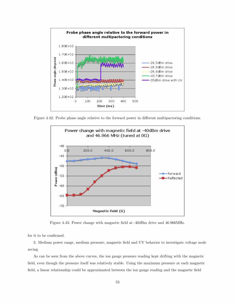
Figure 4.42: Probe phase angle relative to the forward power in different multipactoring conditions.
Figure 4.43: Power change with magnetic field at -40dBm drive and 46.966MHz.
for it to be confirmed.
3. Medium power range, medium pressure, magnetic field and UV behavior to investigate voltage node
arcing
As can be seen from the above curves, the ion gauge pressure reading kept drifting with the magnetic
field, even though the pressure itself was relatively stable. Using the maximum pressure at each magnetic
field, a linear relationship could be approximated between the ion gauge reading and the magnetic field
53
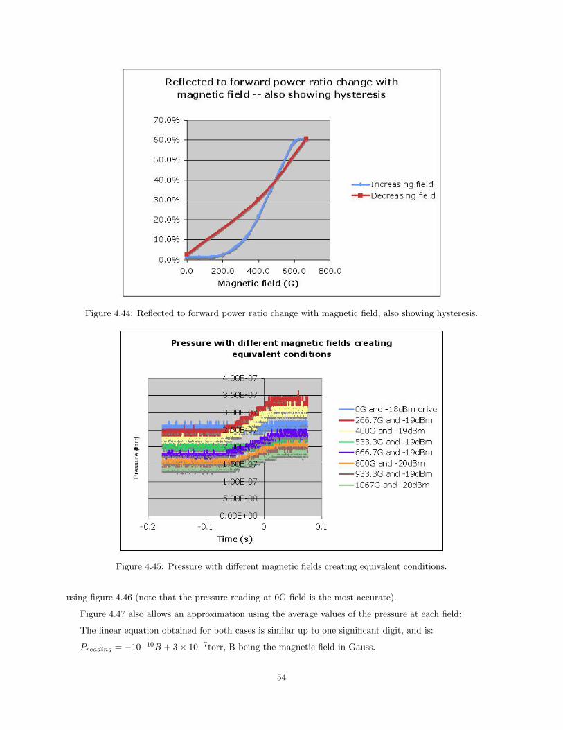
Figure 4.44: Reflected to forward power ratio change with magnetic field, also showing hysteresis.
Figure 4.45: Pressure with different magnetic fields creating equivalent conditions.
using figure 4.46 (note that the pressure reading at 0G field is the most accurate).
Figure 4.47 also allows an approximation using the average values of the pressure at each field:
The linear equation obtained for both cases is similar up to one significant digit, and is:
Preading = −10−10B + 3× 10⁻⁷torr, B being the magnetic field in Gauss.
54

Figure 4.46: Maximum ion gauge pressure reading change with magnetic field.
Figure 4.47: Average ion gauge pressure reading change with magnetic field.
These equivalent conditions occur when the voltage at the probe is between -34.2 and -35.3dBm, and
the phase angle difference with the forward power 138◦ to 152◦. In this case the base pressure was at
55

Figure 4.48: DC bias with different magnetic fields created equivalent conditions.
2.1× 10⁻⁷torr.
Figure 4.49: DC bias with different magnetic fields resulting in similar conditions.
In this case, the equivalent conditions are when the voltage at the probe is between -36.5 and -38dBm,
and the phase angle difference with the forward power 138◦ to 143◦. In this case the H2 pressure was
raised to 1.4× 10⁻⁵torr.
An event worth noting is that the UV multipactor happening at -33dBm drive seemed to be suppressed
by a magnetic field, such as 133.3G, and disappeared with the application of 200G and higher. Figure 4.50
shows the comparative states of the forward power, reflected power, probe signal, and the DC bias at the
inner conductor of the transmission line during this event.
The breaks that are observed in figure 4.50 happen at 34 of the way through the RF pulse, and
56

Figure 4.50: Multipacoring with magnetic field and UV radiation present.
correspond to the initiation of the UV pulse. As can be seen, besides the slight decrease in the probe signal
and slight increase in the reflected signal caused by the increase of 133.3G in the magnetic field, not much
else is different. The average values can be viewed in 4.8:
On 7/27/07, six conditions were examined: multipactor at different magnetic fields at 1.2× 10⁻⁴torr
pressure, arc at 1.1× 10⁻⁴torr pressure, and plasma at different magnetic fields at 4.7× 10⁻⁴torr pressure.
The comparison graphs can be seen in figure 4.51:
The forward power for the arc rises to as high as 4900W, and averages at 2080W. The magnetic field
generally seems to cause an increase (or an upward drift) in the forward power. The forward power seems
to be generally more stable in the presence of plasma than multipactor (or it is possible that the amplitude
change has to do more with the magnitude of power).
The arcs maximum reflected power is 1160W, and the average reflected power is 588W. The plasma
57
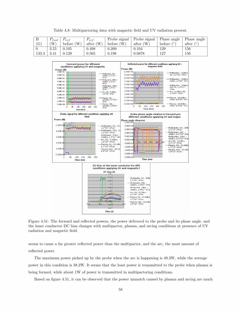
Table 4.8: Multipactoring data with magnetic field and UV radiation present.
B Pfwd Pref Pref Probe signal Probe signal Phase angle Phase angle(G) (W) before (W) after (W) before (W) after (W) before (◦) after (◦)0 3.55 0.105 0.498 0.209 0.104 129 156133.3 3.41 0.129 0.565 0.198 0.0878 127 156
Figure 4.51: The forward and reflected powers, the power delivered to the probe and its phase angle, andthe inner conductor DC bias changes with multipactor, plasma, and arcing conditions at presence of UVradiation and magnetic field.
seems to cause a far greater reflected power than the multipactor, and the arc, the most amount of
reflected power.
The maximum power picked up by the probe when the arc is happening is 49.3W, while the average
power in this condition is 38.2W. It seems that the least power is transmitted to the probe when plasma is
being formed, while about 1W of power is transmitted in multipactoring conditions.
Based on figure 4.51, it can be observed that the power unmatch caused by plasma and arcing are much
58

greater than the unmatch caused by multipactor. Also, arcing delivers considerably higher power to the
electrodes.
One thing to note is that the analog ion gauge reading seems to not have been working (even though at
the time it was not noticed on the oscilloscope, so it might actually be a data acquisition software
problem). It may also be because of a sudden increase in pressure. While the digital reader might have
been reset after such an occurrence, the analog was not.
4.3 Error analysis
4.3.1 Statistical error
The standard error for these experiments was calculated by dividing the the standard deviation of the
sample by the square root of the sample size:
SDx =σ√n
(4.6)
where σ is the standard deviation of the sample obtained by:
σ =
√√√√ 1
N
N∑i=1
(xi − µ)2. (4.7)
Where µ is the mean and N is the sample size.
4.3.2 Systematic and random error
The measured and true value are related by: where σ is the standard deviation of the sample obtained by:
x = T + ε+ ∆ (4.8)
Where ε account for the random uncertainty or the precision or the repeatability error of the
experiment and ∆ is the systematic uncertainty or the bias in the experiment.
The random errors being introduced in these experiments were from difficulty of controlling having the
exact pressure and temperature when the breakdowns happened. Also, though surfaces were thouroughly
cleaned and rinsed with the acetone, IPA, DI, IPA procedure more than once, any insluble surface
pollutants might have introduced random errors and caused electric breakdown. There could have been a
multitude of other random errors such as contamination of the vacuum by pump oil vapors or particles
from the sandpaper adhering to the surface of the electrode.
59

Systematic errors included the accuracy of the instruments used. The micrometer used had an accuracy
of ±1µm. Surface analysis experiments performed outside of clean room environment have a tendency to
include another variety of systematic errors as the surfaces get introduced to air which can carry various
particles that can attach themselves to the surface. Care was taken to minimize these by doing the rinse
procedure before placing the electrodes in the vacuum and blowing high pressure N2 on them, however, the
contamination elimination of these techniques are limited.
60
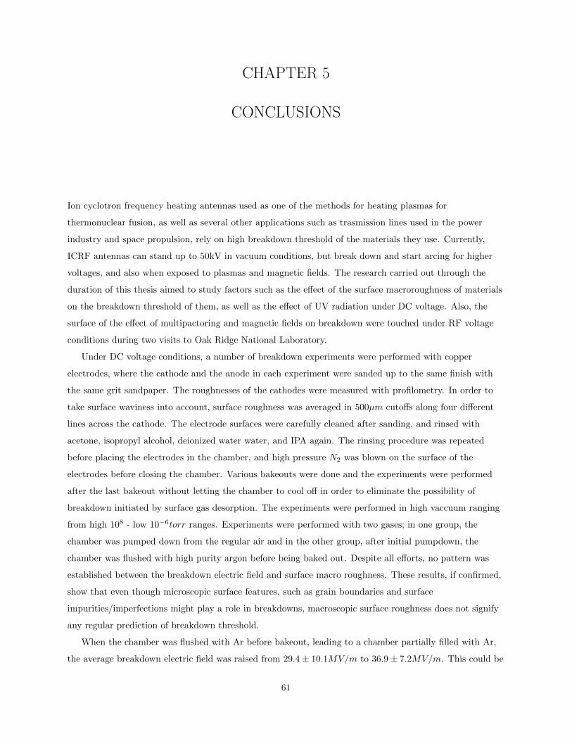
CHAPTER 5
CONCLUSIONS
Ion cyclotron frequency heating antennas used as one of the methods for heating plasmas for
thermonuclear fusion, as well as several other applications such as trasmission lines used in the power
industry and space propulsion, rely on high breakdown threshold of the materials they use. Currently,
ICRF antennas can stand up to 50kV in vacuum conditions, but break down and start arcing for higher
voltages, and also when exposed to plasmas and magnetic fields. The research carried out through the
duration of this thesis aimed to study factors such as the effect of the surface macroroughness of materials
on the breakdown threshold of them, as well as the effect of UV radiation under DC voltage. Also, the
surface of the effect of multipactoring and magnetic fields on breakdown were touched under RF voltage
conditions during two visits to Oak Ridge National Laboratory.
Under DC voltage conditions, a number of breakdown experiments were performed with copper
electrodes, where the cathode and the anode in each experiment were sanded up to the same finish with
the same grit sandpaper. The roughnesses of the cathodes were measured with profilometry. In order to
take surface waviness into account, surface roughness was averaged in 500µm cutoffs along four different
lines across the cathode. The electrode surfaces were carefully cleaned after sanding, and rinsed with
acetone, isopropyl alcohol, deionized water water, and IPA again. The rinsing procedure was repeated
before placing the electrodes in the chamber, and high pressure N2 was blown on the surface of the
electrodes before closing the chamber. Various bakeouts were done and the experiments were performed
after the last bakeout without letting the chamber to cool off in order to eliminate the possibility of
breakdown initiated by surface gas desorption. The experiments were performed in high vaccuum ranging
from high 108 - low 10−6torr ranges. Experiments were performed with two gases; in one group, the
chamber was pumped down from the regular air and in the other group, after initial pumpdown, the
chamber was flushed with high purity argon before being baked out. Despite all efforts, no pattern was
established between the breakdown electric field and surface macro roughness. These results, if confirmed,
show that even though microscopic surface features, such as grain boundaries and surface
impurities/imperfections might play a role in breakdowns, macroscopic surface roughness does not signify
any regular prediction of breakdown threshold.
When the chamber was flushed with Ar before bakeout, leading to a chamber partially filled with Ar,
the average breakdown electric field was raised from 29.4± 10.1MV/m to 36.9± 7.2MV/m. This could be
61

due to different work function of combined metal-gas system in each case. Interestingly, Hackam and
Raju [15] have suggested that for different gases different breakdown mechanisms are at work at the same
gap length. However, since the uncertainty in the data is greater than the differnce in the mean values, it
is impossible to draw a final conclusion. Further experiments would be needed to confirm or refute the
combined metal-gas system work function effect on breakdown mechanism and threshold.
In the case of aluminum cathodes with varying roughness used in conjunction with electropolished
semi-spherical copper anodes whose roughness was kept constant in various experiments, UV light was
shown to decrease the breakdown threshold from 62.5± 11.5MV/m to 50.2± 17.7MV/m, consistent with
the assumption that photoemission also plays a role in causing breakdowns. However, once again, due to
the large standard deviations, the difference in the means is not large enough to surpass the uncertainty in
measurement, hence making a final conclusion postponsed until further, independent experiments are
performed in the future.
At ORNL, using a high-speed camera to capture the kinds of breakdown encountered in an RF
tramission line and then extracting the frames helped to distinguish them into three types: 1) ”Emission”
or ”glow”, where electrons are suspected to be accelerated through material because of the high electric
field, colliding with the copper atoms and heating them up, and causing them to emit light. 2) ”Arc”,
explained by the electric field being so high that the copper ions accelerate across the electrodes, creating
these arcs. 3) Plasma, which was created at sections of transmission line other than the electrode tips.
This phenomenon occured with every pulse at higher powers and higher pressures, and even at low powers
with high pressure and the appropriate matching frequency. It was also possible to get the phenomena of
both stages 2 and 3, when there was an arc as well as a plasma present in the chamber.
Initial studies comparing the forward and reflected power in an RF transmission line leading to two
electrodes in different conditions including initiation of multipactor, arcing, and plasma revealed that
plasma seems to cause a far greater reflected power than multipactoring, while the arc causes the most
amount of reflected power. Also, power unmatch caused by plasma and arcing are much greater than the
unmatch caused by multipactor. Additionally, arcing delivers considerably higher power to the electrodes.
These observations need to be confirmed by further studies.
62

CHAPTER 6
FUTURE WORK
There is still a long road ahead in determining the macro and micro factors that influence a breakdown in
the vaccuum, and how to affect the breakdown threshold.
6.1 DC experiments
One thing that was not studied but would be nice to know was in case of anode and cathode that were
made of different materials, what kind of material transfer could be expected between the electrode. This
could be studied given various data points where both the anode and the cathode were studied using EDS
following one virgin electrode breakdown. This could be even further studied if the cathode was made of a
point tip electrode, and vice versa.
In order to refine the Ar flushed experiments, it would perhaps help to flush the chamber for a more
prolonged amount of time, and bring the Ar pressure up to about 10−3 − 10−2 before pumping down again.
This may help to lower the range of breakdown voltage data for Ar and reduce the uncertainty by reducing
the standard deviation of the data, in order for the difference in average breakdown threshold to be more
conclusive.
Another recommendation is for to try to perform the experiments in a clean room. The reason is, no
matter how finely the electrodes are cleaned before being put into the chamber, it is impossible to
eliminate all debris on their surface right before closing off the chamber after putting them in by virtue of
being exposed to regular air. In a clean room, much more accurate results may be achieved by having the
microparticle breakdown initiation mechanism join the control factors.
As for cleaning the electrodes, other methods may be tried before using them in the chamber. The
electrodes were cleaned using detergent wash after sading, and afterwards acetone, IPA, DI water, and IPA
rinse, once immediately after and once right before putting in the chamber. The sequence was immitated
after what is also common in semiconductor IC production. Ultrasonic cleaning in acetone was also tried in
a few cases. However, in the future, other methods such as acid (e.g. HF) rinse may be tried before
proceeding to the normal rinse as well. This would especially be helpful if it was used in conjunction with
a clean room.
For future roughness experiments, the author would consider a full range of experiments with constant
63

roughness anode (electropolished, e.g.) and variable roughness cathode, both with copper and aluminum to
compare with the results discussed in this thesis. Also, as an alternative to Ar flushing, the chamber could
be rinsed with dry air (instead of the ”laboratory” air) to prevent having variable humidity for each
experiment. Also, running a glow discharge in the chamber after flushing it with any gas may be more
suitable to make sure the chamber has been properly flushed and the new gas is now the dominant one in
the chamber. Once low enough uncertainties can be reached in the data, other gases may be tried as well,
most importantly helium, hydrogen, and nitrogen, as some of the most relevant gases in the vicinity of
tokamaks.
In order to understand the effect of temperature on the breakdown thresholds, the electrodes should be
heated to a certain temperature and steadily kept there, so the electrode distance can become a control
factor. Halogen lamps as used in these experiments are not suitable for keeping the lamps at a certain
steady temperature. Once a steady temperature that would not longer contribute to change of distance
between electrodes is achieved, the effects or significance of change in thermal emission on breakdown
threshold can be studied.
Breakdown studies of other materials and some coatings, especially those available around a
thermonuclear fusion plasma which may come into contact with the ICRF antennas would also be of
interest. Study of the effect of different magnetic fields on breakdown thresholds is also of great importance
given the structure of a tokamak.
6.2 RF experiments
Further experiments are certainly needed to establish the breakdown mechanism as well as the events
leading to breakdown in electrodes under RF voltage, as they will help in determining the voltage
withstanding threshold of ICRF antennas as well as other applications. More experiments with finely
controlled control factors are needed to be able to predict a breakdown as it approaches.
The effect of electrode surface roughness in an RF environment is something else that might be
considered. Thought the DC setting did not show a clear depenence on electrode surface macroroughness
and the breakdown threshold, an RF setting may show different results.
Given that emission, arcing, and plasma were sighted across the electrodes and in the trasmission line,
a spectrometer could be placed at the window to study the light from emission and arcing, to determine
what materials are present, and whether the surface material is also evaporating or it is just the gas in the
chamber being ionized. This can also be repeated with the DC experiments, especially if the two electrodes
are from different materials, to determine whether the anode or the cathode is being evaporated more, if at
all. This would in turn help greatly to determine whether these DC breakdowns are anode or cathode
initiated.
64

APPENDIX A
model.m
%{
Model.m calculates the reflection coefficient of the breakdown tester
antenna, as well as the voltage and current at each point of the antenna.
The inputs are two files:
1. characterstics.xls which contains the information about the coaxial
sections of the antenna.
2. The file that contains the reflection coefficient measured data for
the purposes of comparison.
The outputs are four plots of the reflection coefficient and the voltage
vs. length graph, as well the file testdata.csv, which contains the
frequencies as well as the real and imaginary components of the measured
reflection coefficient.
The functions used in this program are the following:
inducatance.m, capacitance.m, resistance.m, gamma.m, Zchar.m, impedance.m,
ZofCap.m, RFLcoeff.m, voltage.m, current.m.
Author: Maro Aghazarian <[email protected]>
%}
clear
% Every value used in this file is in metric units, except for values of f
% (frequency), which are in MHz.
% The input is going to contain a matrix with three columns representing
% the input frequencies, real part of the reflection coefficent, and the
% imaginary part of the reflection coefficient respectively.
65

expRFL = xlsread(’smallRange.xls’);
freqNum = size (expRFL, 1);
% This file is going to contain a number_of_coax_cables x 7 matrix, the
% columns containing inside radius, outside radius, relative permeability of the
% dielectric, relative permittivity of the dielectric, resistance coefficient of the
% inside material, resistance coefficient of the outside material, and the
% length of the coaxial cable with these characteristics, respectively.
chars = xlsread(’characteristics2.xls’);
coaxNum = size(chars, 1);
indcap = zeros(2, coaxNum); % matrix for keeping the inductance and
% conductance for each coaxial cable
data = zeros(5, coaxNum, freqNum); % matrix to store resistance, conductance,
% propagation constant,
% characteristic and load
% impedances.
% Electrode impedance calculation:
Rend = 10^-9;
Cend = 3.615*10^-12;
Zelec = zeros(freqNum);
for i=1:freqNum
Zelec(i) = complex(Rend, -1/(2*pi*expRFL(i)*10^6*Cend));
end
% Coaxial cable section calculations:
for i=1:coaxNum
indcap(1, i) = inductance(chars(i,3), chars(i,1), chars(i,2));
indcap(2, i) = capacitance(chars(i,4), chars(i,1), chars(i,2));
for j=1:freqNum
data(1, i, j) = resistance(expRFL(j), chars(i,1), chars(i,2), chars(i,5),+
->chars(i,6));
data(2, i, j) = 0; % conductance
omega = 2*pi*10^6*expRFL(j);
data(3, i, j) = gamma(omega, data(1,i,j), indcap(1,i), data(2,i,j), indcap(2,+
66

->i));
data(4, i, j) = Zchar(omega, data(1,i,j), indcap(1,i), data(2,i,j), indcap(2,+
->i));
if (i==1)
Zload = Zelec(j);
else
Zload = data(5, i-1, j);
end
data(5, i, j) = impedance(data(4,i,j), Zload, data(3,i,j), chars(i,7));
end
end % end of the coaxial cable section calculations
% Calculating the impedances of the capacitors and the line sections in the box.
% constants of the capacitors:
Lshunt = 92*10^(-9);
Cshunt = 131.67*10^(-12);
Lseries = 96*10^(-9);
Cseries = 74*10^(-12);
Lcrossin = 0;
Ccrossin = 8.2*10^(-12);
Lstray = 0;
Cstray = 2*10^(-12);
% constants of the line sections:
wcapin = 0.065;
hcapin = 0.055;
xcapin = 0.15;
fcapin = 0.18;
Dcross = 0.4525;
dcross = 0.065;
xcross = 0.2794;
fcross = 0.6;
rinnerin = 0.015;
routerin = 0.0345;
Z0in = 50;
xin = 0.519;
67

inMat = 1;
outMat = 1;
% initializing the arrays
Zshunt = zeros(freqNum);
Zseries = zeros(freqNum);
Zcrossin = zeros(freqNum);
Zstray = zeros(freqNum);
Zcross = zeros(freqNum);
Zcapin = zeros(freqNum);
gammacross = zeros(freqNum);
gammacapin = zeros(freqNum);
gammain = zeros(freqNum);
Zin = zeros(freqNum);
% line section initial calculations
Cspeed = 2.9979*10^8; % speed of light in vacuum
Z0capin = 377*(hcapin/wcapin)*fcapin; % lossless
Lcapin = Z0capin/Cspeed;
Ccapin = 1/(Z0capin*Cspeed);
p = Dcross/dcross;
A_cross = (1 + 0.405*p^-4)/(1 - 0.405*p^-4);
B_cross = (1 + 0.405*p^-8)/(1 - 0.405*p^-8);
C_cross = (1 + 0.405*p^-12)/(1 - 0.405*p^-12);
Z0cross = (138*log10(p) + 6.48 - 2.34*A_cross - 0.48*B_cross - 0.12*C_cross)*fcross; % +
->lossless
Lcross = Z0cross/Cspeed;
Ccross = 1/(Z0cross*Cspeed);
Lin = Z0in/Cspeed;
Cin = 1/(Z0in*Cspeed);
for m=1:freqNum
% capacitor characteristic impedances
omega = 2*pi*expRFL(m)*10^6;
Zshunt(m) = ZofCap(omega, Lshunt, Cshunt, 0.001*(expRFL(m)^(1/2)));
Zseries(m) = ZofCap(omega, Lseries, Cseries, 0.001*(expRFL(m)^(1/2)));
68

Zcrossin(m) = ZofCap(omega, Lcrossin, Ccrossin, 0);
Zstray(m) = ZofCap(omega, Lstray, Cstray, 0);
% line section characteristic impedances
Rgen = 0.1*(expRFL(m)^(1/2));
Rin = 3*resistance(expRFL(m), rinnerin, routerin, inMat, outMat);
Zcross(m) = Zchar(omega, Rgen, Lcross, 0, Ccross);
Zcapin(m) = Zchar(omega, Rgen, Lcapin, 0, Ccapin);
Zin(m) = 50;
%Zchar(omega, Rin, Lin, 0, Cin);
gammacross(m) = gamma(omega, Rgen, Lcross, 0, Ccross);
gammacapin(m) = gamma(omega, Rgen, Lcapin, 0, Ccapin);
gammain(m) = gamma(omega, Rin, Lin, 0, Cin);
end % end of capacitor and line impedance calculations
% Integrating the results and calculating the reflection coefficient:
Zint = zeros(9, freqNum); % Will hold the impedances at the junctions,
% assumed to be 9.
rho = zeros(freqNum);
for j=1:freqNum
Zint(1, j) = (data(5, coaxNum, j)*Zshunt(j)) / (data(5, coaxNum, j)+Zshunt(j));
Zint(2, j) = impedance(Zcross(j), Zint(1, j), gammacross(j), xcross*3/4);
Zint(3, j) = (Zint(2,j)*Zcrossin(j)) / (Zint(2,j)+Zcrossin(j));
Zint(4, j) = impedance(Zcross(j), Zint(3,j), gammacross(j), xcross*(1/4));
Zint(5, j) = (Zint(4,j)*Zstray(j)) / (Zint(4,j)+Zstray(j));
Zint(6, j) = Zint(5,j) + Zseries(j);
Zint(7, j) = (Zint(6,j)*Zstray(j)) / (Zint(6,j)+Zstray(j));
Zint(8, j) = impedance(Zcapin(j), Zint(7,j), gammacapin(j), xcapin);
Zint(9, j) = impedance(Zin(j), Zint(8,j), gammain(j), xin);
rho(j) = RFLcoeff(Zin(j), Zint(9,j));
end
% calculating the magnitude of the reflection coefficient at each point.
rhoMag = zeros(freqNum, 1);
exp = zeros(freqNum);
69

for i=1:freqNum
rhoMag(i,1) = abs(rho(i,1));
exp(i) = sqrt((expRFL(freqNum+i))^2+(expRFL(freqNum*2+i))^2);
% abs(complex(expRFL(freqNum+1:freqNum*2),expRFL(freqNum*2+1:freqNum*3)
% ));
end
%Plotting and recording the data
d(1:freqNum,1)=real(rho(1:freqNum,1));
d(1:freqNum,2)=imag(rho(1:freqNum,1));
subplot (2,2,1)
plot(expRFL(1:freqNum),exp(1:freqNum),expRFL(1:freqNum),rhoMag(1:freqNum,1))
title(’Magnitude of the Reflection Coefficient’)
legend(’input’,’calculated’)
subplot (2,2,2)
plot(expRFL(freqNum+1:freqNum*2),expRFL(freqNum*2+1:freqNum*3),d(1:freqNum,1),d(1:+
->freqNum,2))
title(’Imaginary Component vs. Real Component of the Reflection Coefficient’)
legend(’input’,’calculated’)
subplot (2,2,3)
plot(expRFL(1:freqNum),atan2(expRFL(freqNum*2+1:freqNum*3),expRFL(freqNum+1:freqNum*2)))
hold on
plot(expRFL(1:freqNum),atan2(d(1:freqNum,2),d(1:freqNum,1)),’color’,[1,0.4,0.6])
title(’Phase Angle of the Reflection Coefficient’)
legend(’input’,’calculated’);
hold off
xlswrite(’testdata’, d(1:freqNum,1:2))
% Calculating the voltage and the current at each point of the antenna
% reuturns the minimum magnitude of the reflection coefficent, as well as
% the index of it (which would give us the minimum frequency through expRFL(index))
[resonance, index] = min(rhoMag(1:freqNum,1));
70

% constants
sectionNum = 13; % number of the coaxial cable sections all throughout the antenna
nummax = 50; % number of the regions each section is devided to for analysis
% initializing
Velec = 1;
Ielec = Velec/Zelec(index);
results = zeros(sectionNum*nummax, 3); % this matrix will hold the voltage, current,
% and total length of the antenna to a point.
% it consists of sectionNum*nummax rows,
% and three columns for V, I, and L
% respectively.
for i = 1:sectionNum
if i==1
V = Velec;
I = Ielec;
Z0 = data(4, 1, index);
gamma = data(3, 1, index);
Lreg = chars(1, 7);
elseif i>coaxNum
if i==coaxNum+1 % this is the region parallel with shunt capacitor
V = results((i-1)*nummax, 1);
I = results((i-1)*nummax, 2) + results((i-1)*nummax, 1)/Zshunt(index);
Z0 = Zcross(index);
gamma = gammacross(index);
Lreg = xcross*0.75;
elseif i==coaxNum+2
V = results((i-1)*nummax, 1);
% Zcrossin was substituted for Zstray
I = results((i-1)*nummax, 2) + results((i-1)*nummax, 1)/Zcrossin(index);
Z0 = Zcross(index);
gamma = gammacross(index);
Lreg = xcross*0.25;
elseif i==coaxNum+3
V = results((i-1)*nummax, 1) + results((i-1)*nummax, 2)*Zseries(index);
71

I = results((i-1)*nummax, 2);
Z0 = Zcapin(index);
gamma = gammacapin(index);
Lreg = xcapin;
end
else
V = results((i-1)*nummax, 1); % voltage of end of the previous homogeneous +
->section
I = results((i-1)*nummax, 2); % current of end of the previous homogeneous +
->section
Z0 = data(4, i, index);
gamma = data(3, i, index);
Lreg = chars(i, 7);
end
for j = 1:nummax
section = ((i-1)*nummax+j);
Lsec = -1*j/nummax*Lreg;
results(section, 1) = voltage(V, I, Z0, gamma, Lsec);
results(section, 2) = current(V, I, Z0, gamma, Lsec);
if (section-1)==0
results(section, 3) = chars(i, 7)/nummax;
else
results(section, 3) = results(section-1, 3) + Lreg/nummax;
end
end
end
% Calculating the factor for graphing the results
Zinput = results(sectionNum*nummax,1)/results(sectionNum*nummax,2);
Pin = 2000;
Iin = (Pin/real(Zinput))^(1/2);
Vin = Iin*Zinput;
subplot(2,2,4)
plot(results(1:sectionNum*nummax,3), abs(Vin*results(1:sectionNum*nummax,1))/abs(results+
->(sectionNum*nummax,1)))
72

title(’Voltage vs. Length of the Antenna’)
inductance.m
%Filename: inductance.m
%This function calculates the inductance.
%Inputs are: relative permeability constant miu, inner radius of the coaxial cable,
%and the outer radius of the coaxial cable in identical metric units.
function f = inductance(miu, Rin, Rout)
f = miu*4*pi*10^(-7)/(2*pi)*log(Rout/Rin);
capacitance.m
%Filename: capacitance.m
%This function calculates the capacitance.
%Inputs are: relative permittivity constant epsilon, inner radius of the coaxial cable,
%and the outer radius of the coaxial cable in identical metric units.
function f = capacitance(epsilon, Rin, Rout)
f = (2*pi*epsilon*8.8541878176*10^-12)/log(Rout/Rin);
resistance.m
%Filename: resistance.m
%This function calculates the resistance of the transmission line.
%Inputs are: frequency of the signal in the region in MHz, inner radius, outer
%radius, inner material resistance coefficient, and outer material
%resistance coefficient.
function f = resistance(freq, Rin, Rout, inMat, outMat)
Rscale = .596;
f = Rscale*((2.61*10^-4)/(2*pi))*(freq)^(1/2)*(inMat/Rin + outMat/Rout);
gamma.m
73

%Filename: gamma.m
%This function calculates the propagation constant.
%Inputs are: frequency in radians, resistance, inductance,
%conductance, and capacitance.
function g = gamma(omega, R, L, G, C)
g = ((R + omega*i*L)*(G + i*omega*C))^(1/2);
Zchar.m
%Filename: Zchar.m
%This function calculates the propagation constant.
%Inputs are: frequency in radians, resistance, inductance,
%conductance, and capacitance.
function f = Zchar(omega, R, L, G, C)
f = ((R + omega*i*L)/(G + i*omega*C))^(1/2);
impedance.m
%Filename:impedance.m
%This function calculates the load impedance.
%Inputs are: characteristic impedance of the region, load impedance at the
%end of the previous region, propagation constant, and length of the
%region.
function f = impedance(Z0, Zl, gamma, length)
f = Z0*(Zl*cosh(gamma*length)+Z0*sinh(gamma*length))/(Z0*cosh(gamma*length)+Zl*sinh(+
->gamma*length));
ZofCap.m
%Filename: ZofCap.m
%This function calculates the load impedance of the capacitors.
%Inputs are: the frequency in radian, the inductance in Henries, the
%capacitance in Farads, and the resistance in ohms.
74

function f = ZofCap(omega, L, C, R)
f = complex(R, (omega*L - 1/(omega*C)));
RFLcoeff.m
%Filename: RFLcoeff.m
%This function calculates the reflection coefficient.
%Inputs are: characteristic impedance and the load impedance of the region.
function f = RFLcoeff(Z0, Zl)
f = (Zl - Z0)/(Zl + Z0);
voltage.m
%Filename: voltage.m
%This function calculates the voltage along the antenna.
%Inputs are: voltage at the end of the previous homogeneous region, current at the end
%of previous homorgeneous region, the characteristic impedance of the current +
->homogeneous region,
%the propagation constant of the current homogeneous region, and the negative length
%from the beginning of the current homogeneous region.
function f = voltage(Vprev, Iprev, Z0, gamma, length)
f = Vprev*cosh(gamma*length) - Iprev*Z0*sinh(gamma*length);
current.m
%Filename: current.m
%This function calculates the voltage along the antenna.
%Inputs are: voltage at the end of the previous homogeneous region, current at the end
%of previous homorgeneous region, the characteristic impedance of the current +
->homogeneous region,
%the propagation constant of the current homogeneous region, and the negative length
%from the beginning of the current homogeneous region.
75

function f = current(Vprev, Iprev, Z0, gamma, length)
f = Iprev*cosh(gamma*length) - Vprev*sinh(gamma*length)/Z0;
76

APPENDIX B
tempCalc.m
clear
avgPower = input(’Please enter the average power of each pulse (kW): ’)
avgDelay = input(’Please enter the average delay between pulses(s): ’)
pointNum = input(’Please enter the number of data points taken in this run: ’)
avgTime = input(’Please enter the average time you spent at each point(min): ’)
% constants:
coaxLength = 1.495; %m
coaxVolume = 0.001667691; %m^3
elecVolume = 0.00002011; %m^3
Delec = 0.0254; %diameter of the electrode in meters
Lelec = 0.04445; %length of the electrode in meters
Cu_density = 8920; %kg/m
pulsetime = 45; %ms
specHeatCu = 0.386; %J/(g.C)
alphaCu = 17.6*10^-6; % Cu linear expansion coefficient in 1/C or 1/K
permittivity = 8.8541878176*10^-12; %F/m
gap = 0.9; %mm
mass = (coaxVolume + elecVolume)*Cu_density;
delQ = pulsetime*avgPower*pointNum*avgTime*floor(60/avgDelay)/1000;
delT = delQ/(specHeatCu*mass)
%centigrades
delL = (alphaCu*(coaxLength+Delec)*delT)*100
%cm
77

delLelec = (alphaCu*Lelec*delT)*1000; % mm
delC = permittivity*10^3*(1/(gap-delLelec)-1/gap)*10^9
%nF
78

APPENDIX C
RoughAnalysis.m
%{
RoughAnalysis takes Excel files containing surface height data from
profilometry that contain five columns of data, following each other
from left to right and then downward, as well as how small of a scale
we want to divide the data (usually across 5000Mm or 5mm) and analyze
separately (e.g. 50Mm, 200Mm, etc.). Afterwards, it divides the data to
corresponding segments, uses linear regression to find the slope of the
surface of the electrode, and using that flattens the data to be able
to compute exactly the roughness of the surface. Then it averages the
roughness of mentioned scale across all segments and outputs it to a file.
The functions used in this program are the following:
Author: Maro Aghazarian <[email protected]>
%}
clear
% Every value used in this file is in metric units.
% The input is an excel file containing surface height data in five columns
% and many rows that follow each other from left to right and then top to
% bottom.
SurfaceHeight = xlsread(’example.xlsx’);
SurfRows = size(SurfaceHeight, 1);
SurfCols = size(SurfaceHeight, 2);
datapoints = SurfRows*SurfCols;
79

% Length of the reading of profilomentry (Sclen). Usually 5000 or 10000Mm.
length = 10000;
x_inc = length/(datapoints-1); % x step increments
x = zeros(datapoints, 1); % one column vector containing all x values
y = zeros(datapoints, 1); % one column vector containing all y values
for i=0:SurfRows-1
for j=1:SurfCols
if i+j==1
x(1) = 0;
y(1) = SurfaceHeight(1,1);
else
x(j+i*5)= x(j+i*5-1)+x_inc;
% puts all values in SurfaceHeight in single vector
y(j+i*5)=SurfaceHeight(i+1,j);
end
end
end
%SegLength = input(’How long do you want each segment to be? (Mm) ’);
% input segment length
AllSegLength = [2.5 5 10 20 50 100 200 250 500 1000 2000 2500];
AllRa = zeros(1,10);
AllRq = zeros(1,10);
for mm=1:12;
SegLength = AllSegLength(mm);
SegNum = length/SegLength; % Number of segments
yNum = datapoints/SegNum; % Number of datapoints of each segment
% new y calculated after flattening the curve with linear regression
y_new = zeros(yNum, SegNum); % will include y after linear regression
% linear regression thou art biutiful!
for i=1:SegNum
80

sigmaY = 0;
sigmaX = 0;
sigmaX2 = 0;
sigmaXY = 0;
a = 0;
b = 0;
position=(i-1)*yNum;
for k=1:yNum
sigmaY = sigmaY+y(k+position);
sigmaX2 = sigmaX2+(x(k+position)^2);
sigmaX = sigmaX+x(k+position);
sigmaXY = sigmaXY+y(k+position)*x(k+position);
end
a = (sigmaY*sigmaX2-sigmaX*sigmaXY)/(yNum*sigmaX2-sigmaX^2);
b = (yNum*sigmaXY-sigmaX*sigmaY)/(yNum*sigmaX2-sigmaX^2);
for j=1:yNum
y_new(j,i)=y(position+j)-(a+b*x(position+j));
end
end
% trying to put y_new from a yNum x SegNum matrix into a datapoints x 1
% array so I can write it to excel more easily
y_new_organizaed=zeros(datapoints,1);
for ii=1:SegNum
y_new_organized((ii-1)*yNum+1:ii*yNum,1)=y_new(1:yNum,ii:ii);
end
% Calculating roughness of each segment!
Roughness=zeros(SegNum,3); % columns will contain Ra, Rq, Rz for each segment
for i=1:SegNum
sigmaY = 0;
sigmaY2 = 0;
for j=1:yNum
sigmaY=sigmaY+abs(y_new(j,i));
81

sigmaY2=sigmaY2+y_new(j,i)^2;
end
Roughness(i,1)=1/yNum*sigmaY; % assigning Ra of each segment
Roughness(i,2)=sqrt(1/yNum*sigmaY2); % assigning Rq of each segment
end
R_sum = sum(Roughness,1);
Ra = 1/SegNum*R_sum(1,1);
Rq = 1/SegNum*R_sum(1,2);
AllRa(1,mm) = Ra;
AllRq(1,mm) = Rq;
end
% excel output
xlswrite(’AllRoughness’,AllSegLength,’A1:L1’);
xlswrite(’AllRoughness’,AllRa,’A2:L2’);
xlswrite(’AllRoughness’,AllRq,’A3:L3’);
82

REFERENCES
[1] V. Bergeaud, L.G. Eriksson, and D.F.H. Start. Iter relevant icrf heating scenarios with large ionheating fraction. Nuclear Fusion, 40(1):35–51, 2000.
[2] R. A. Cairns. Radiofrequency Heating of Plasmas. IOP Publishing Ltd., 1991.
[3] Carlos Henry Castano. Study of Breakdown/Arcing for High Power RF Antennas on FusionApplications. PhD thesis, University of Illinois at Urbana-Champaign, Urbana, IL, 2006.
[4] J.B.O. Caughman, C. Castano-Giraldo, M. Aghazarian, F.W. Baity, D.A. Rasmussen, and D.N.Ruzic. Study of rf breakdown mechanisms relevant to an ich antenna environment. Proceedings of the17th Topical Conference on Radio Frequency Power in Plasmas, 17, 2007.
[5] J.B.O. Caughman, C. Castano-Giraldo, M. Aghazarian, F.W. Baity, D.A. Rasmussen, and D.N.Ruzic. Study of rf breakdown mechanisms relevant to and ich antenna environment. Proceedings ofthe 17th Topical Conference on Radio Frequency Power in Plasmas, 17, 2007.
[6] Christopher Coleman. An Introduction to Radio Frequency Engineering. Cambridge University Press,2004.
[7] Lawrence Cranberg. The initiation of electrical breakdown in vacuum. Journal of Applied Physics,23(5):518–522, 1952.
[8] F. Durodie, Ph. Chappuis, J. Fanthome, R.H. Goulding, J. Hosea, P.U. Lamalle, A. Lorenz, M.P.S.Nightingale, L. Semeraro, and F. Wesner. Main design features and challenges of the iter-like icrfantenna for jet. In Proceedings of the 23rd Symposium of Fusion Energy - SOFT 23, pages 223–228,Madison, WI, 2005.
[9] P. Erdos. Thermionic emission. In McGraw-Hill Encyclopedia of Science and Technology, pages288–289. McGraw-Hill, Inc., U.S.A.
[10] F. Hohn et al. The transition of a multipactor to a low-pressure gas discharge. Physics of Plasmas,4(4), April 1997.
[11] Elise Fourre, Philippe Jean-Baptiste, Arnaud Dapoignya, Dominique Baumiera, Jean-Robert Petit,and Jean Jouzel. Past and recent tritium levels in arctic and antarctic polar caps. Physics of Plasmas,4(4), 2006.
[12] I. N. Golovin. Prospects for the practical use of controlled fusion with magnetic plasma confinement.Soviet Journal of Plasma Physics, 16(12), 1990.
[13] T. P. Graves. Experimental Investigation of Electron Multipactor Discharges at Very High Frequency.PhD Thesis. MIT, 2006.
[14] T.P. Graves. Command Reference Manua. MIT, 2006.
[15] Reuben Hackam and G.R. Govinda Raju. Electrical breakdown of a pointplane gap in high vacuumand with variation of pressure in the range 10−710−2 torr of air, nitrogen, helium, sulphurhexafluoride, and argon. Journal of Applied Physics, 45(11), 1974.
83
[16] A.M. Howatson. An Introduction to Gas Discharges. Pergamon Press Ltd., Oxford, England, 1965.
[17] Karl Jousten. Handbook of Vacuum Technology. Wiley-VCH.
[18] Karl Jousten. Thermal outgassing. 28 May - 3 Jun 1999.
[19] R.H. Good Jr. and E.W. Muller. Field emission. In Encyclopedia of Physics, pages 176–231.Springer-Verlag, Germany.
[20] Kaye and Laby. Tables of Physical and Chemical Contents. 16th ed. Longman Sc and Tech online,1995.
[21] E. Kuffel and W.S. Zaengl. High Voltage Engineering Fundamentals. Pergamon Press.
[22] Rod Latham. High Voltage Vacuum Insulation: Basic Concepts and Technological Practice. AcademicPress Inc., 1995.
[23] Rod Latham. High Voltage Vacuum Insulation: A New Perspective. AuthorHouse, Bloomington, IN,2006.
[24] I.S. Lehrman, P.L. Colestock, D.H. McNeill, G.J. Greene, S. Bernabei, J.C. Hosea, M. Ono, J.L.Shohet, and J.R. Wilson. Edge measurements during icrf heating on the plt tokamak. Plasma Physicsand Controlled Fusion, 32(1):51–71, 1990.
[25] David R. Lide. Radiofrequency Heating of Plasmas. CRC online, 2007.
[26] M.A. Lieberman and A.J. Lichtenberg. Principles of Plasma Discharges and Materials Processing.John Wiley and Sons, Inc., U.S.A., 2005.
[27] W.B. Nottingham. Thermionic emission. In Encyclopedia of Physics, pages 1–175. Springer-Verlag,Germany.
[28] K. Oura, V.G. Lifshits, A.A. Saranin, A.V. Zotov, and M. Katayama. Surface Science: AnIntroduction. Springer, Germany, 2003.
[29] Dektak3ST Surface Profile Measuring System. Installation, Operation, and Maintenance Manual.Veeco Sloan Technology Division, 2006.
84