eindhoven university of technology master strategic and
TRANSCRIPT

Eindhoven University of Technology
MASTER
Strategic and tactical decision making in a dedicated transportation service in the chemicalcluster of Rotterdama business model
van de Bunt, L.G.
Award date:2015
Link to publication
DisclaimerThis document contains a student thesis (bachelor's or master's), as authored by a student at Eindhoven University of Technology. Studenttheses are made available in the TU/e repository upon obtaining the required degree. The grade received is not published on the documentas presented in the repository. The required complexity or quality of research of student theses may vary by program, and the requiredminimum study period may vary in duration.
General rightsCopyright and moral rights for the publications made accessible in the public portal are retained by the authors and/or other copyright ownersand it is a condition of accessing publications that users recognise and abide by the legal requirements associated with these rights.
• Users may download and print one copy of any publication from the public portal for the purpose of private study or research. • You may not further distribute the material or use it for any profit-making activity or commercial gain

Eindhoven, August 2015
identity number 0857799
in partial fulfilment of the requirements for the degree of
Master of Science
in Operations Management and Logistics
Supervisors:
Prof. dr. ir. J.C. Fransoo, TU/e, OPAC
Dr. ir. M. Udenio, TU/e, OPAC
Dr. ir. J. Aerts, Den Hartogh Logistics
Strategic and tactical decision making
in a dedicated transportation service
in the chemical cluster of Rotterdam –
A business model*
*Public version: No names of companies are used and monetary
amounts are scaled
by
Luke (L.G.) van de Bunt

ii
TUE. School of Industrial Engineering. Series Master Thesis Operations Management and Logistics
Subject headings: business case, resource-based view, linear programming, simulation, logistics,
transportation, chemical industry

iii
Contents Abstract ................................................................................................................................................... v
List of Abbreviations .............................................................................................................................. vi
Management Summary ........................................................................................................................ vii
Preface ................................................................................................................................................... xi
1. Introduction .................................................................................................................................... 1
1.1. Problem statement ................................................................................................................. 1
1.2. Case description: Transportation within a chemical cluster ................................................... 2
1.3. Literature review ..................................................................................................................... 3
1.4. Research questions ................................................................................................................. 6
1.5. Methodology ........................................................................................................................... 6
1.6. Thesis outline .......................................................................................................................... 7
2. Resource-based view model ........................................................................................................... 8
2.1. Selection procedure ................................................................................................................ 9
2.2. Strategic Industry Factors ....................................................................................................... 9
2.3. Strategic Cluster Factors ....................................................................................................... 15
2.4. Strategic resources of the cluster service ............................................................................. 16
2.5. Business Strategy .................................................................................................................. 18
3. Cluster service calculation model ................................................................................................. 21
3.1. Conceptual design ................................................................................................................. 21
3.2. Basic model design ................................................................................................................ 23
3.3. Detailed design ..................................................................................................................... 29
4. Business case analysis ................................................................................................................... 40
4.1. Cost structure ........................................................................................................................ 40
4.2. Market price .......................................................................................................................... 42
4.3. AsIs results ............................................................................................................................ 42
4.4. Demand scenarios ................................................................................................................. 43
4.5. Main drivers business case ................................................................................................... 46
4.6. Robustness ............................................................................................................................ 48
4.7. Discussion .............................................................................................................................. 49
5. Conclusions & Recommendations ................................................................................................ 51
5.1. Conclusions ........................................................................................................................... 51
5.2. Recommendations ................................................................................................................ 52
5.3. Further research ................................................................................................................... 53

iv
Appendix 1: RFP/RFQ procedure .......................................................................................................... 55
Appendix 2: Complaints ........................................................................................................................ 56
Appendix 3: Near misses and accidents ................................................................................................ 57
Appendix 4: Information flow cluster service ....................................................................................... 58
Appendix 5: Typical cluster demand ..................................................................................................... 59
Appendix 6: Cluster nodes and chemical facilities ................................................................................ 60
Appendix 7: Transportation distance .................................................................................................... 61
Appendix 8: Cluster node and chemical facility time ........................................................................... 62
Appendix 9: Verification of basic model ............................................................................................... 63
Appendix 10: Combining groups of different fixed/flexible ratios ....................................................... 66
Appendix 11: Determining matching probabilities ............................................................................... 67
Appendix 12: Cost structure ................................................................................................................. 69
Appendix 13: Terminal allocation ......................................................................................................... 70
Appendix 14: Scenario result overview ................................................................................................ 71
Appendix 15: Cluster demand overlap analysis .................................................................................... 72
Bibliography .......................................................................................................................................... 74

v
Abstract This report describes the business case of a new dedicated transportation service of Den Hartogh
Logistics, a chemical logistic service provider (LSP), in the chemical cluster of Rotterdam. This cluster
service solely transports chemical tank containers within the Rotterdam Port area and competes
with smaller, regional LSPs. Typically, these smaller LSPs are cheaper due to lower overhead costs
and a more flexible operation. Hence, from a resource-based view (RBV) perspective, we identify
other market factors than price on which the cluster service has the potential to compete. Next, by
means of an optimization model, we calculate the gap between the cluster service price and the
price of the smaller LSPs. To overcome this price gap, economies of scale and the transportation
flexibility of the cluster volumes are identified as main drivers to reduce cost of the cluster service.

vi
List of Abbreviations
3PL Third-Party Logistics Provider
AIMMS Advanced Integrated Multidimensional Modeling Software
D/S Drop-Swap
IO Industrial Organization
ISO International Organization for Standardization
KPI Key Performance Indicator
KSF Key Success Factor
LNG Liquefied Natural Gas
LSP Logistic Service Provider
OTIF On-Time-In-Full
RFI Request For Information
RFP Request For Proposal
RFQ Request for Quotation
RBV Resource-Based View
SCF Strategic Cluster Factor
SIF Strategic Industry Factor
SQAS Safety & Quality Assessment System
VBA Visual Basic for Applications
VRIN Value, Rare, Inimitable and Non-substitutable
VRP Vehicle Routing Problem

vii
Management Summary In this report we present the results of a master thesis conducted at Den Hartogh Logistics. Den
Hartogh is a logistic service provider (LSP) within the chemical industry and transports bulk
chemicals. Although Den Hartogh is globally active, the major of its business is still located in one of
the largest chemical cluster in the world, the Port of Rotterdam.
Problem statement
Large inefficiencies occur within the chemical cluster of Rotterdam due to fixed loading and
unloading times at the chemical producers. First of all, these fixed moments highly restrict the
transportation planning of chemical LSPs. Furthermore, LSPs are forced to introduce slack in the
arrival times of trucks to avoid late arrivals. Trucks therefore have to wait most of the times before
being serviced at the chemical producers.
Consequently, these inefficiencies make transportation more expensive. Typically, short
transportation flows within and just outside the cluster of Rotterdam are outsourced by Den
Hartogh to smaller, less expensive, LSPs. However, as Den Hartogh wants to strengthen its market
position in the cluster of Rotterdam, the company is interested in identifying the opportunities to
compete with these smaller LSPs.
Because the smaller LSPs are able to offer a lower transport price, Den Hartogh has to compete on
other market demand factors than costs. If the strategy turns out to be successful, cluster volumes
are expected to increase. Due to economies of scale, the cluster service of Den Hartogh may even
reach a critical mass to become price competitive.
To find a solution for the described problem statement, we first identified the opportunities, threats
and design of the cluster service in case of both a price disadvantage and a price advantage. These
aspects are described in a business strategy. In the second part of the study, we designed a
calculation model which identified the critical mass of the cluster service to become price
competitive. A combination of the two parts can be formulated in the following question:
What is the business case of a dedicated transportation service in the cluster of Rotterdam?
Business strategy
Based on the resource-based view (RBV) theory, we formulated a business strategy for the cluster
service. The goal of this business strategy is to describe how a competitive advantage can be created
by providing transportation services within the cluster of Rotterdam.
First of all, the business strategy includes the opportunities for the cluster service to compete in the
market. Through semi-structured interviews with different market players, price, quality and safety
were identified as most important opportunities. However, the perceptions of their relative
importance were different among the customers. We therefore decided to divide the customers into
two customer classes: (1) collaborative customers and (2) transactional customers. Collaborative
customers are willing to invest in long-term improvement projects on quality and safety whereas
transactional customers valued low transportation prices as most important.

viii
Secondly, the business strategy identifies threats which could have a negative impact on the
competitive position of the cluster service. To start, several interviewees identified a monopoly
position as a potential threat. On the other hand, most of them also recognized the market would
not to accept such a position. Next, opportunistic behavior by Den Hartogh was perceived as a
serious threat. In the cluster service, Den Hartogh will not only transport its own, but also tank
containers of other LSPs. Therefore, Den Hartogh has the opportunity to give priority to its own
equipment. Lastly, information accessibility was mentioned as a potential threat. Currently,
information about the destination and which LSP performs the transportation demand is very
sensitive to customers. However, since Den Hartogh will also transport tank containers of other LSPs,
this information needs to become available by transportation documents.
Thirdly, the business strategy proposes a cluster service design based on its resources. According to
the RBV theory, these resources have the potential to create a competitive advantage when they
comply with the opportunities and threats, and when they are rare (i.e. not widely available in the
market). In case of the cluster service, drivers and the cluster network are identified as important
resources. Well-trained and experienced drivers have the potential to positively impact quality and
safety of cluster transportations, and a strong (i.e. with high volumes and balanced) network has the
potential to positively impact the price of cluster transportations.
Finally, a two-phase business strategy was formulated. The first phase, the so-called ‘start-up’ phase,
represents the current situation of the cluster service (i.e. volumes of the cluster service are low and
price is high). Hence, only volumes of collaborative customers were identified as potential demand
for the cluster service. Because collaborative customers valued safety and quality as very important,
drivers have to be highly trained and be specialized on the cluster activities. Furthermore, due to the
small size of the cluster service, the effect of the threats on the competitiveness was expected to be
limited. In the second phase, the so-called ‘maturity’ phase, cluster volumes reached a critical mass,
resulting into competitive transportation prices. Not only volumes of collaborative customers were
identified as potential demand for the cluster, but also volumes of transactional customers. On the
other hand, the effect of the threats on the competitiveness of the service was expected to be
significant in this phase. To overcome the problems of information accessibility and opportunistic
behavior, the strategy proposes to set up an independent party to provide the cluster service.
Calculation model
The goal of the calculation model is to calculate the critical mass of the cluster service (i.e. the
transition point between the start-up and maturity phase). Consequently, we were able to
determine the amount of demand from collaborative customers necessary to overcome the gap of
the current cluster service price and the market price.
Typically, a cluster service demand starts with a pickup in the cluster and ends with a drop in the
cluster. An optimization model was developed to minimize the total cluster service time to execute
the daily demand. The output of this model is dependent on the repositioning decision of a truck
between two consecutive demands. If the truck is required to reposition between two different
locations, the truck has to drive so-called solo kilometers and has to wait in line with other trucks to
pick up the new tank container. However, if no repositioning is required, and the pickup location
‘matches’ the previous drop location, solo transportation time and waiting time can be neglected.

ix
AsIs Scenario 1 Scenario 2 Scenario 3 Scenario 4
Cluster service price €12.85 €12.67 €12.20 €11.97 €11.89
Market price €12.50 €12.50 €12.50 €12.50 €12.50
€11.40
€11.60
€11.80
€12.00
€12.20
€12.40
€12.60
€12.80
€13.00
Pri
ce/h
ou
r
Cluster service rate vs. market rate
€-
€2.00
€4.00
€6.00
€8.00
€10.00
€12.00
€14.00
Total cluster servicecosts
Market price
Co
st/h
ou
r
Margin
Front- andback-officecostIT cost
Fuel cost
Chassis cost
Plannercost
Truck cost
Subsequently, we determined the matching probabilities of two consecutive demands and used
these as input to our optimization model. The matching probabilities are dependent on the number
of pickups and drops at a cluster location, whether these drops and pickups are balanced and their
fixed/flexible ratio. Whether a drop or pickup is flexible or fixed depends on the type of cluster
demand. A fixed demand has no planning freedom and is fixed to a certain moment of the day (i.e.
slot bookings to load/unload at chemical producers) and a flexible demand has a certain degree of
planning freedom and is therefore not fixed to a certain moment of the day (i.e. a transportation
between a terminal and depot).
Finally, a simulation program was designed to approach the stochastic behavior of the demands. 200
demands scenarios were created and solved by the optimization model.
Business case
To determine gap between the current cluster price and the market price, the cluster service price
per hour was determined based on the result of the calculation model (see figure 1a). As turned out,
the cluster service is 2.8% (i.e. €11.550 on a yearly base) more expensive compared to the market
price. Based on the business strategy, we identified the collaborative shippers and their potential
demand in the cluster. Subsequently, we created four potential future demand scenarios and
calculated their effect on the cluster service price (see figure 1b). In scenario 2, with a flexible
demand increase of 3825 tank containers (59%) per year and a fixed increase of 750 tank containers
(28%) per year, the cluster becomes price competitive.
Figure 1a: Structure cluster service price Figure 1b: Cluster service price vs. market price in 4 scenarios
Insights
Increases in demand volume mainly drive the cost reductions in every scenario. Fixed costs are
allocated over more hours, which results in a lower cost per hour. On the other hand, the increase in
matching probabilities appeared to be low. Hence, the impact on the cluster service price was
marginal. The low increase in matching probabilities was explained by the high initial probabilities in
the AsIs situation. Subsequently, these high matching probabilities were caused by large numbers of
flexible demands.

x
Recommendations
1) Although the gap of 2.8% seems small, the cluster service should strengthen its market
position by increasing its volumes with demand of collaborative customers instead of
offering a competitive price to commit transactional customers.
2) In the start-up phase, the cluster service should focus on potential flexible demands at
collaborative shippers. These flexible demands are created by the so-called ‘drop-swap’
operations (i.e. buffer locations before the tank containers are loaded or unloaded).
3) Good commercial skills are necessary in the start-up phase of the cluster service.
4) Introduce a reward system to steer the allocation of demands over the cluster nodes.
xi
Preface Rotterdam, August 17th 2015
This report is the final result of my master thesis project at Den Hartogh Logistics. But, above all, the
end of six amazing years as a student. I started my student life at the University of Groningen, where
I met great people, enjoyed being active at the study association and learned a lot during my study.
After finishing the bachelor Industrial Engineering and Management in 4 years, I decided to
exchange the ‘Martinitoren’ for the ‘Catharinakerk’. I enjoyed my time in Eindhoven and I am proud
being graduated from the master program Operations Management and Logistics. However, I will
never change my green-white shirt for a red-white one.
Next, I would like to thank several people who were indispensable in the process to reach the end
result of this master thesis. First of all, I would like to thank Joep Aerts for giving me the opportunity
to graduate at Den Hartogh Logistics. Joep, you inspired me with your unlimited amount of
enthusiasm, and your creative and smart way of thinking. Furthermore, thank you for not only being
my supervisor, but also for letting me experience the important aspects of being a practitioner.
Secondly, I would like to thank my supervisor at the University of Eindhoven, Jan Fransoo. I really
learned a lot from our discussions on conceptual thinking. Where I sometimes tended to get lost in
details, you pulled me up and let me think in the bigger picture. I also would like to thank Maxi as my
second supervisor. Maxi, although you were my second supervisor, I really appreciated our frequent
meetings and your 100% availability. Especially in the beginning, when I had some start-up
problems, you helped me by providing the structure of thinking in small steps instead of trying to
overlook the whole research from the start.
Thirdly, I would like to thank all people at Den Hartogh Logistics who helped me with getting familiar
with the company and its processes. I had a great time spending my days at the office in Rotterdam.
Special thanks to Marius Bouwens, for patiently answering all my questions about tender procedures
and selection criteria of chemical producers. Also special thanks to Jacco van Holten, for our
discussions and helping me get in contact with several stakeholders in the chemical industry. Finally,
I am Gerrit Vis and Nils van der Poel grateful for helping me to gather data for the calculation model.
Last, but definitely not least, I would like to thank my family, friends and lovely girlfriend. Their
unconditional support during my study and this project was indispensable. I really appreciate them
for always being there for me.

1
1. Introduction
1.1. Problem statement
In this report we present the results of a master thesis conducted at Den Hartogh Logistics. Den
Hartogh is a logistic service provider (LSP) within the chemical industry and transports bulk chemicals
in tank containers. The LSP is headquartered in Rotterdam and has access to its own fleet of more
than 4000 tank containers, 400 road barrels and 500 trucks. Although Den Hartogh is globally active,
the center of demand gravity is located in one of the largest chemical cluster in the world, the Port
of Rotterdam.
Because large inefficiencies occur within the chemical cluster of Rotterdam, we scope down to the
transportation activities of Den Hartogh in this area. Inefficiencies are primarily caused by fixed
loading and unloading times at the chemical producers. First of all, these fixed moments highly
restrict the transportation planning of chemical LSPs. Furthermore, LSPs are forced to introduce
slack in the arrival times of trucks to avoid late arrivals. Trucks therefore have to wait most of the
times before being serviced at the chemical producers.
Consequently, these inefficiencies make transportation expensive. Typically, short transportation
flows within and just outside the cluster of Rotterdam are outsourced by Den Hartogh to smaller,
less expensive, LSPs. Because these LSPs are active in a small region, they are more flexible.
Furthermore, because they are smaller and do not have own tank containers, overhead costs are
significantly lower.
However, Den Hartogh wants to strengthen its market position in the cluster of Rotterdam and is
therefore interested in identifying the opportunities to compete with these smaller LSPs. Because
the smaller LSPs are able to offer a lower transport price, Den Hartogh has to compete on other
market demand factors than costs. If this strategy turns out to be beneficial, cluster volumes are
expected to increase. Due to economies of scale, the cluster service of Den Hartogh may even reach
a critical mass to become price competitive.
Based on this problem description we split our study into two parts. In the first part we identified
the competitive advantage of the cluster service in case of a price disadvantage and a price
advantage. In the second part of the study we designed a calculation model which identified the
critical mass of the cluster service to become price competitive.
A combination of the two parts can be formulated in the following question:
What is the business case of a dedicated transportation service in the cluster of Rotterdam?
The remainder of the chapter is organized as follows. First, we shortly described the chemical cluster
of Rotterdam and chemical transportation in more detail in section 1.2. Then, in section 1.3, we
discussed a theoretical model which enables us to identify a competitive advantage by the resource-
based view (RBV). In section 1.4, based on the problem statement and the results of the literature
review, we formulated the research questions. The methodology used to answer the research
questions is discussed in section 1.5. Finally, in section 1.6, an outline of the thesis is provided.

2
Containers
Storage liquid bulk
Dry bulk
Distribution
Chemistry/Refineries/Energy
Other
1.2. Case description: Transportation within a chemical cluster
Clusters are “geographic concentrations of firms, suppliers, support services, specialized
infrastructure, producers of related products, and specialized institutions (e.g., training programs
and business associations) that arise in particular fields in particular locations.” (Porter, 2007, p. 1)
The amount, size and diversity of clusters are getting larger because their influence on competition
is growing (Porter, 2007). They play a fundamental role in knowledge creation, innovation,
accumulation of skills, and development of pools of employees with specialized expertise.
1.2.1. Chemical cluster of Rotterdam
With more than 45 chemical companies and 5 refineries1, together responsible for producing 13
million tonne of products per year2, the Port of Rotterdam is one of the world’s largest oil and
chemical clusters.
Figure 1.1: Chemical cluster of
Rotterdam
As a result, large volumes of chemical products are entering and leaving the chemical cluster,
typically by tank containers. The transportation of these tank containers are performed by trucks,
trains and ships.
On the other hand, also transportation flows within the cluster of Rotterdam are significant. Mainly
because the infrastructure of rail and waterways are not flexible enough to reach most locations in
the cluster, last or first mile transportation has to be performed by truck. Hence, if an empty tank
container has to be loaded and arrives by ship or train at a terminal (i.e. a facility where containers
are transshipped between different transport modalities), a truck will pick up the tank container,
drives it to the chemical facility, waits until the tank container is loaded, and drops the tank
container at a terminal again. This sequence of transportation activities is perceived as a typical
cluster transportation flow.
1.2.2. Chemical cluster transportation
In the chemical industry, most products are transported by third-party logistics service providers
(3PL). Hence, transportation between the chemical producer and its customer is outsourced to
another party. The company that sends the product is called ‘shipper’, and the company that
1 http://www.portofrotterdam.com/en/business/chemicals/Pages/chemicals.aspx 2 http://www.portofrotterdam.com/en/News/pressreleases-news/Documents/Your_chemical_port_of_choice-PDF_tcm26-20160.pdf
3
transports the product is called ‘carrier’. Both the customer as the supplier of the chemical products
can fulfill the role of shipper, and therefore take responsibility of contracting carriers.
Tender procedure
Typically, shippers work together with multiple carriers. Carriers are selected by shippers through
tendering. To shippers, the goal of a tender is to get an idea about the expected performance of a
carrier on, for example, price, on-time deliveries, responsiveness, etc. In most cases, shipper and
carrier will agree upon a contract for 1-3 years, based on the expected amount of products to be
transported and the agreed performance of the carrier.
Tank operators vs. trucking operators
Between LSPs in the chemical industry, a distinction can be made between tank operators and
trucking operators. Tank operators, like Den Hartogh, are characterized by a large pool of trucks and
employees, own tank containers and a large transportation network. On the other hand, trucking
operators are small, do not have own tank containers and are primarily active in a small region. Due
to these characteristics, shippers do not invite trucking operators to a tender. Instead, trucking
operators are the suppliers of tank operators at short, regional transportation flows or during
periods of limited truck capacity. Due to the low overhead cost and high flexibility, trucking
operators are able to offer short transportation flows at a lower price. Whereas only tank operators
are invited by shippers in the tender procedure, these operators are referred to ‘carriers’.
As mentioned in the problem statement, Den Hartogh is interested in identifying opportunities to
compete with trucking operators in the cluster of Rotterdam. However, because trucking operators
are able to offer a lower transport price, Den Hartogh has to compete on other market demand
factors than costs. In the next section we elaborate, in a short literature review, on the theoretical
model that was used to identify these factors.
1.3. Literature review
In this section, we reviewed a theoretical model which is not only able to identify the factors which
have the potential to create a competitive advantage, but also which company resources contributes
most to these factors. This model is based on the resource-based view (RBV). For a complete
literature review regarding the resource-based view in logistics, the reader is referred to Van de
Bunt (2014).
1.3.1. Resource-based view
The resource-based view (RBV) was developed to complete a shortcoming of industrial organization
(IO) economics (i.e. structure->conduct->performance paradigm) by Porter (1980; 1981; 1985). In
the IO view Porter suggested two central strategic issues for achieving high profitability:
(1) Industry selection, based on the five forces model;
(2) Strategy selection (cost leadership, product differentiation or focus), to remain a
competitive position within the industry.
However, these issues put the determinants of firm performance outside the firm and are not
challenging the question why firms in the same industry might differ in performance. Based on the
work of Penrose (1959), strategic management and marketing scholars (Amit & Schoemaker, 1993;

4
Barney, 1991; Peteraf, 1993; Rumelt, 1987; Wernerfelt, 1984) proposed a resource-based
explanation of firm and performance heterogeneity. Rather than being defined by the parameters of
a firm’s competitive environment, the parameters of a firm’s competitive strategy are critically
influenced by its accumulated resources (Barney, 1991). According to Wernerfelt (1984), Barney
(1991) and Peteraf (1993) these resources become possible sources for competitive advantage and
will lead to above-normal returns.
1.3.2. Definition of a resource
According to Barney (1991; 2002), firm resources include “all assets, capabilities, organizational
processes, firm attributes, information, knowledge, etc. controlled by a firm that enable the firm to
conceive of and implement strategies that improve its efficiency and effectiveness” (Barney, 1991, p.
101; 2002, p. 155). Although this definition is widely used in literature, it is also a highly criticized
aspect of the RBV. The critique of Priem and Butler (2001), which states this definition is overly
inclusive, plays a key role in this discussing.
The overly inclusiveness of the resource definition includes that everything strategically associated
with a firm could be a resource. Kraaijenbrink et al. (2010) stated that this over-inclusiveness is a
problem for two reasons: (1) The definitions do not sufficiently acknowledge the difference between
resources that are inputs to the firm or capabilities the firm uses to select, deploy, and organize such
inputs and (2) the definition does not address fundamental differences in how different types of
resources may contribute in a different manner to a firm’s competitive advantage.
To overcome the problems of overly inclusiveness, we use the definition of Van de Bunt (2014)
where resources are “all input resources and capabilities of a firm that may have been developed
inside the firm or acquired in the market” (Van de Bunt, 2014, p. 4).
1.3.3. VRIN criteria
When Barney (1991) introduced the resource-based view, he stated that resources which are
common to all firms or easily available in the marketplace cannot provide a competitive position.
Only resources that meet the conditions of being valuable, rare, inimitable and non-substitutable
(VRIN) can endow a company with a competitive advantage (Amit & Schoemaker, 1993; Barney,
1991).
Valuable: Resources are considered valuable when they enable a firm to conceive of or
implement strategies that improve performance, exploit market opportunities or neutralize
impeding (Barney, 1991, 1995).
Rare: Resources are rare when only utilized by the firm itself or to the firm and a few
competitors (Coates & McDermott, 2002; Olavarrieta & Ellinger, 1997).
Inimitable: Three general isolating mechanisms prevent the imitation of resources and
capabilities: property rights, learning and development costs, and causal ambiguity (Hoopes,
Madsen, & Walker, 2003; Lippman & Rumelt, 1982; Rumelt, 1987). Property rights apply
most directly on resources. Learning and development costs on resources and capabilities.
Causal ambiguity on capabilities.

5
Non-substitutable: Resources are imperfectly substitutable when equivalent resources from
a strategic point of view do not exist (Coates & McDermott, 2002).
From these four criteria, three have some similarities. Rareness, inimitability and non-substitutability
all seem to stress the scarcity of the resource. This was also noticed by Hoopes et al. (2003) who
made the statement that the rareness-criteria is only relevant when a resource is valuable and
cannot be imitated or substituted by competitors. Otherwise both rareness and imitability or
rareness and substitutability would measure the same kind of scarcity.
1.3.4. Value of a resource
Amit and Schoemaker (1993) introduced an interesting model, which was later adjusted by Van de
Bunt (2014) (see figure 1.2), to determine the value of a resource. The foundation of their model is
based on an empirical, ex post test of the longstanding strategy premise (Vasconcellos & Hambrick,
1989) that an organization’s success depends on the match between its strengths and the Key
Success Factors (KSF) in its environment. Using a range of mature industrial product industries, their
empirical findings showed that organizations which rated highest on industry KSF clearly
outperformed their rivals. Amit and Schoemaker subsequently argued that the resources from the
RBV and the industrial factors from the IO-perspective correspond with the strength of the firm and
the industry KSF, respectively. This resulted in a model where value of resources is derived from the
amount of overlapping and convergence between “strategic assets” and “strategic industry factors”.
Figure 1.2: The source of competitive advantage adjusted from Amit and Schoemaker (1993)
Strategic assets coincide with the resources at the firm level according to the RBV. So the
challenge facing a firm is to identify a set of strategic assets as grounds for establishing the
firm’s sustainable competitive advantage. According to Amit and Schoemaker (1993), the
sustainable competitive advantage opportunity of these strategic assets, depends on their
own characteristics as well as on the extent to which they overlap with the industry-
determined Strategic Industry Factors.
Strategic Industry Factors (SIFs) coincide with resources and competencies at the
industry/market level. Thus they characterize all the firms that possess them, and explain
their success with respect to other industries/markets (Toni & Tonchia, 2003). By definition,

6
SIFs are determined through complex interactions among the firm’s competitors, customers,
regulators, innovators external to the industry and other stakeholders. It is important to
recognize that the relevant set of SIFs changes and cannot be predicted with certainty ex
ante (Amit & Schoemaker, 1993).
1.4. Research questions
As already indicated in the problem statement, this study is split up into two parts. In the first part,
based on the RBV, we investigated the competitive advantage of the cluster service in case of a price
disadvantage and a price advantage. In the second part, we discussed the critical volumes from
which the cluster service is able to compete on price. Based on this structure, the research questions
were formulated:
1. Is the cluster service able to create a competitive advantage in the chemical cluster of
Rotterdam?
1.1. What are the Strategic Industry Factors (SIFs) in the chemical cluster of Rotterdam?
1.2. What is the relative importance of the SIFs in the chemical cluster of Rotterdam?
1.3. Which resources are used in the cluster service?
1.4. Which of the identified resources are strategic and which are non-strategic?
The second part of the study is divided into two research questions. Based on the first research
question we designed the calculation model which should be able to determine the critical mass
and, based on the second research question, the actual business case of the cluster service was
developed.
2. How should the calculation model be designed to calculate the business case of the cluster
service?
3. What is the business case of the cluster service?
1.5. Methodology
Based on the nature of the problem, i.e. determining the business case of the cluster service, we
formulated the problem as a practical problem. Therefore, the research was conducted in the form
of a case study. Consequently, problem is ‘unique’, instead of general, and was therefore handled as
a design, instead of a knowledge problem (Van Aken, 1994). Van Aken (2004) described the
reflective cycle as the methodology to be used to solve unique problems from practice.

7
Case class selection
Case selection
Regulativecycle
Reflection on results
Determination of design
knowlegde
Identification of a problem
Diagnosis
Plan of actionIntervention
EvaluationReflective cycle Regulative cycle
Figure 1.3: The reflective cycle (Van Aken, 2004)
RBV model
In the first part of the study, we used the RBV model to determine the competitiveness of the cluster
service without cost advantage. The results are primarily based semi-structured interviews with
participants from the chemical industry. Additionally, we use the mixed-method to confirm or
disconfirm the beliefs and feelings of participants during interviews (Woodside, 2010). Hence, we
used participant observation and document analysis.
Calculation model
Although the regulative cycle is covering the complete research, Bertrand and Fransoo (2002)
identified a relevant research methodology in quantitative modeling in operations management.
Bertrand and Fransoo distinguished between axiomatic and empirical, and descriptive and
normative research methodologies. Our study is more consistent with empirical research as only the
output of the model is relevant for our findings, rather than the insights into the structure of the
model itself. Furthermore, the study fits better with descriptive research as we wanted to know how
changes in parameters influenced the output of the model.
According to Bertrand and Fransoo (2002), the
model of Mitroff et al. (1974) can be used in
designing a quantitative model. Typically, ED
research, the researcher follows a cycle of
“conceptualization-modeling-validation”. This cycle
replaces the steps ‘plan of action’ and
‘intervention’ in the regulative model.
Figure 1.4: Model of Mitroff et al. (1974)
1.6. Thesis outline
The thesis is organized as follows: In chapter 2, we discussed the implementation of the RBV model.
Next, the design of the calculation model was elaborated in chapter 3. In chapter 4, based on the
findings of the RBV model, future demand scenarios where formulated. Subsequently, the price
competitiveness of each scenario was determined by the calculation model. Finally, in chapter 5, the
conclusions and recommendations were presented.

8
2. Resource-based view model In this chapter, we determined a business strategy for the cluster service. The goal of this business
strategy is to describe how to create a competitive advantage in providing transportation services
within the cluster. The business strategy considers two phases: In the first phase, the strategy is
based on the fact the cluster service has a price disadvantage compared to its competitors.
Furthermore, in the second phase, the strategy is adjusted when the critical volumes are reached
and the price disadvantage disappears. In the formulation of the business strategy, the different
aspects of the RBV model, as discussed in the literature review, are used.
First of all, the proposed strategy identified which market demands the cluster service have to meet
to become competitive. These market demands are represented by the Strategic Industry Factors
(SIFs) of the RBV model. To identify the SIFs, we interviewed 4 shippers, 2 tank operators and 1 truck
operator. As turned out from these interviews, customers use the same set of SIFs, but differ in their
perception about the relative importance. We therefore proposed two different customer classes:
The first class represents the shippers who identified SIFs, other than price, as most important. The
second class represents the shipper who identified price as most important SIF.
Secondly, besides the opportunities to become competitive, the proposed strategy also identifies
potential threats of the cluster service. Because the cluster service changes the current way of
executing a transportation flow (i.e. an additional party and activity is included), the interviewees
also identified several threats as a result of this change. Like the SIFs, these threats are used to
determine the value of the cluster service. We therefore name the threats after the SIFs, namely
Strategic Cluster Factors (SCF).
Thirdly, the proposed strategy identifies the important resources of the cluster service and how they
can contribute to the market demands. Following the logic of the RBV model, we determined the
alignment of the resources with the SIFs and SCFs. The better the resources are aligned, the higher
the customer value. However, as discussed in the literature review, only value is not enough to
determine the competitive advantage. We therefore also analyzed the rareness of the resources.
Finally, we were able to formulate a business strategy which describes the requirements to become
competitive in the ‘start-up phase’ (i.e. low volumes and a price disadvantage) and in the ‘maturity
phase’ (i.e. high volumes and a price advantage) of the cluster service.
As a result from the above mentioned steps, the chapter is organized as follows: Typically, tendering
is used by shippers to select carriers. Hence, by winning a tender, the carrier has a competitive
advantage over other carriers. Selection criteria in a tender procedure are therefore expected to
coincide with the SIFs. We therefore first describe the tender procedure in section 2.1, before
discussing the SIFs in section 2.2. In section 2.3, we describe the SCFs and in section 2.4 we elaborate
on the value and rareness of the cluster service resources. To finalize the chapter, we describe the
business strategy of the cluster service in section 2.5.

9
2.1. Selection procedure
To select the best carriers, shippers typically use a tender procedure. In this tender procedure, the
participating carriers are benchmarked on several selection criteria. The carrier who performs best
on the selection criteria is offered a contract for a period of 1-3 years.
Standard tender procedure
In practice, several types of tender procedures are used. Shippers within the chemical cluster of
Rotterdam mainly use a ‘Request for Proposal (RFP)’ and ‘Request for Quotation (RFQ)’.
Request for Proposal (RFP): A RFP is used when the way of executing a (bundle of) lane(s) is
not prespecified. The shipper wants to use the experience, technical capabilities and
creativity of the carriers to come up with a proposal to improve the current situation.
Request for Quotation (RFQ): A RFQ invites carriers to provide a quote for the provision of
services for a specific lane.
For a typical RFP or RFQ procedure, the reader is referred to Appendix 1. Although the content of
the RFP and RFQ is different, this procedure is applicable on both tender types. Furthermore, not
every RFP/RFQ looks exactly the same to the one presented in Appendix 1. However, according to
the interviewees, this procedure represents the steps most frequently used in a tender procedure.
Another described procedure was a two-stage procedure. A second negotiation round was omitted.
Pre-tender procedure
Prior to the standard tender procedure, most shippers perform a so-called ‘pre-tender’. During this
pre-tender phase, a selection of carriers is made who are allowed to participate at the standard
tender procedure. This pre-selection can be executed without the knowledge of the carriers.
Additionally, a pre-selection can also be based on a ‘Request for Information (RFI). During a RFI,
carriers are not selected on rates, but on company characteristics and capabilities.
Based on the different selection moments of a tender procedure as described above, we were able
to ask our interviewees more directed questions about the SIFs. The results are discussed in the next
section.
2.2. Strategic Industry Factors
In this section, we discuss the SIFs as identified by our interviewees. As turned out, shippers have a
rather consistent way of selecting a carrier. However, the relative importance of the SIFs appeared
to be very differently among these shippers. The SIFs which were identified are safety, price, quality,
sustainability, capacity, proactive behavior, personal match, financial stability, network and
transparency. We divided these SIFs in two main groups: Performance and Organizational criteria.
Furthermore, organizational criteria were subdivided in hard and soft criteria.

10
Strategic Industry Factors (SIFs)
Organizational criteria
Performance criteria
Safety Quality Price Sustainability
Hard criteria Capacity Network Financial stability TransparencySoft criteria Transparency Personal match
Figure 2.1: Strategic industry factors in the chemical transportation industry
2.2.1. Performance criteria
Performance criteria are criteria which evaluate the performance of the carrier’s operation.
However, at the beginning of a collaboration, except for the price, the shipper cannot (exactly)
predict the performance of the carrier. To make sure the expectations of the shipper comply with
reality, shippers highly prefer performance criteria to be quantitatively supported with historical
data. However, not every expectation can be (completely) supported this way. In that case, shippers
have to make their decision on their ‘gut feeling’.
Performance criteria are divided in price, safety, quality and sustainability, and will be discussed in
the remainder of this section.
Price
Especially as a result of the economic crises, the focus of every transportation procurement officer
or department of the shipper is on transportation costs. Because the transportation price is directly
related to the transportation costs, this performance criterion is extremely important during a
tender procedure. However, because most shippers recognize that, on the long run, other factors
can also have an impact on costs, price is usually used as a trade-off factor. Shippers ask themselves:
“How much am I willing to pay extra for a better performance of another selection criterion?”
Safety
A good safety performance is very important for every shipper. Some shippers referred to reputation
damage due to recent safety failures of chemical producers in the Netherlands (e.g. fire in 2011 at a
chemical plant in Moerdijk) and others felt highly responsible for everyone who is working at or for
the business. Hence, shippers try to stress safety as very important operational and organizational
aspect at carriers.
The first step in ensuring a high safety performance at carriers, shippers request the required
certificates. Secondly, safety performance at carriers is measured by the Safety & Quality
Assessment System (SQAS). SQAS is a “system to evaluate the quality, safety, security and
environmental performance of Logistics Service Providers and Chemical Distributors in a uniform
manner by single standardised assessments carried out by independent assessors using a standard

11
questionnaire”3. The scores of carriers on SQAS lie between 0 and 100, and are accessible for every
shipper. On the other hand, carriers cannot view the scores of their competitors. Furthermore,
safety is measured by Key Performance Indicators (KPIs). The KPIs mainly exist of amount of near
misses (i.e. a situation which could have led to an accident), number of accidents and number of
spills. However, at most shippers, near misses are not treated as performance indicators. Instead,
near misses should lead to a safety improvement, and carriers should therefore not be demotivated
to report them.
For some shippers, the results of the above mentioned measurements are sufficient to draw
conclusion from the safety performance of a carrier. Even for a potential new carrier, from whom
the KPI-performances are unknown, the possession of the required certificates and an acceptable
score on the SQAS is sufficient to label the operations of the carrier as ‘safe’. On the other hand,
other shippers think the intrinsic safety attitude of a carrier is just as important. That is, “not only
operating to a safety perspective, but also operating from a safety perspective”. Because it is hard to
get a ‘feeling’ about this safety attitude, especially when dealing with new carriers, shippers use
different non-quantifiable tactics to “closely observe the carriers”. Firstly, shippers use audits to
examine the operations and safety policies of the carrier. Secondly, the shipper invites the carrier
during a tender procedure to introduce the company. During this presentation the proactive attitude
on safety is tested. Thirdly, the shipper observes the attendance and input of a carrier during
important safety workshops, workgroups or conferences (e.g. from the CEFIC, The European
Chemical Industry Council). Lastly, some shippers explicitly ask for improvement programs on safety.
In line with these two perspectives, shippers can be divided on their response to the question if
carriers are competing on safety. Both types of shippers agreed that a carrier should have a certain
minimal performance on safety. The first type of shippers sees this level as a threshold to participate
in the tender and therefore stated that carriers are not competing on safety. The second type of
shippers also demands for a certain performance on safety, but additionally expects some proactive
behavior. These shippers stated that carriers are competing on the capability to continuously
improve on safety.
Quality
Especially when the chemical products are valuable, high quality transportation is very important.
During the interviews, quality was also denoted as ‘performance’ and ‘service’. From a customer
service perspective, shippers deem performance at the customer’s site as a very important aspect of
quality. This performance primarily consist of timely deliveries, delivering the right product and the
right quantities, proper communication skills and behavior of drivers, clean equipment and correct
equipment. The KPI-structure of most shippers is divided in ‘On-Time-In-Full (OTIF)’ loadings and
deliveries, and complaints.
Although the OTIF-measure is very transparent and clear, and measured by every carrier, the
problem lies at the complaint-KPI. Complaints are measured differently among shippers and
therefore also among carriers. Hence, it is hard for shippers to compare different carriers on the
complaint-KPI. Additionally, several shippers indicated not to select on the number of complaints,
but rather on the critical self-reflective and proactive attitude to solve and prevent the complaints.
3 www.sqas.org, accessed on 19th May, 2015

12
However, like mentioned before, a proactive behavior is hard to measure. Techniques to get a
feeling about the performance of (especially a new) carrier is to check market references, introduce
a test period and identifying proactive behavior at company presentations. Market references
include the contact between shippers about the performance of the carriers. However, because of
the lack of transparency and collaboration in the chemical industry, detailed information is seldom
shared.
Although dependent on the value of the product and the perspective of the shipper on customer
intimacy, most interviewed shippers explicitly stated willing to accept a higher price in exchange of a
higher quality. Shippers were, for example, willing to pay a higher price for a better OTIF-
performance, new equipment or better trained drivers. However, in the end, the effect of these
extra payments should be justified.
Sustainability
Although sustainability is currently not creating value, shippers identified sustainability as a selection
criterion. At the moment, this selection criterion is only used to binary label a carrier: “Your
operation is sustainable, or it isn’t”. If the carrier meets the legal (e.g. ISO-regulations) and shipper’s
requirements, the carrier is classified as ‘sustainable’. Shippers are not willing to pay an additional
fee for investments to increase sustainability or reduce congestion. Hence, sustainability is only
dependent on governmental regulations, requirements of powerful supply chain players and
initiatives that are also cost-efficient (e.g. intermodal transportation). On the other hand, almost
every stakeholder in the chemical cluster recognized the importance of sustainability and thinks it
will become more important in the future. Therefore this selection criterion has the potential of
becoming valuable in the future.
2.2.2. Organizational criteria
Organizational criteria are criteria which evaluate the organizational characteristics. These
characteristics usually do not change overnight, but are developed over the years. Organizational
criteria are divided into hard and soft criteria. Hard criteria are easily-quantifiable. These criteria are
applicable on the structure and processes of a carrier. Soft criteria are not or hard quantifiable.
These criteria are applicable on the organizational culture and personal relationship.
Hard organizational criteria
Capacity
Capacity is perceived to be the most important hard organizational criterion. Capacity is
represented in fleet size and is directly linked to flexibility. Because the chemical transportation
market is characterized with dynamic and stochastic demands, which lead to short planning
horizons, carriers are expected to be highly flexible. A carrier with a large fleet size is expected to
be more flexible than a carrier with a small fleet size. Most shippers are willing accept a higher
price for a higher flexibility.
Network
The network of the carrier is important because the carrier is expected to be more flexible in the
regions where the carrier is active. Furthermore, a large network indicates a stable operation.

13
Financial stability
Financial stability guarantees a lower operational risk and gives an indication about the
performance in the market.
Transparency
Shippers perceived transparency as very important. Transparency is however a very generic term
and therefore used for multiple purposes. As most frequently mentioned, transparency is
favored in the operations of the carrier. To keep the operation transparent, shippers expect a
clear and consistent KPI and cost structure, with clear and reliable measuring rules.
Soft organizational criteria
Transparency:
A part of the shippers indicated to prefer carriers who provide openness in the communication
structure. That is, having the possibility to directly contact the desired employee in the company
of the carrier (e.g. driver, planner, account manager, etc.). Furthermore, information sharing was
stated to be important in a transparent relationship. Not only information sharing on an
operational level, but also on a strategic level. These shippers are interested in the long-term
vision of carriers and how this vision can be aligned with the vision of the shipper. Shippers
stated that transparency as a soft organizational criteria is only relevant for carriers who (or
potentially going to) transport significant amounts of products.
Personal match
Some shippers and carriers think a personal match between the purchasing manager of the
shipper and the commercial manager of the carrier is important. This personal match is linked
with trust, reliability and sympathy.
As mentioned in the introduction of this chapter, although roughly all interviewed participants
identified the same set of SIFs, the relative importance of the SIFs is different. We therefore
distinguished between two different customer classes. The first class of customers mainly selects
carriers on price and the second class of customers believes safety and quality is more important.
2.2.3. Customer classes
From the SIF analysis in the previous section, we divide the customers in two classes: transactional
and collaborative shippers.
Transactional shippers
Transactional shippers primarily make decisions on quantifiable selection criteria (like price). Hence,
these criteria can be directly related to the logistic performance. Shippers who mainly select on price
are shippers who are transporting low value products with low margins. An example of a procedure
that mainly selects on price is an ‘online-auction’ tender. During an online auction, every participant
is seeing a constantly decreasing price as a result of lower bids of other participants. The participant
with the lowest bid wins the auction. According to the interviewees, these online-auction tenders
typically appeared as a consequence of the economic crisis in 2008.

14
However, most of the transactional shippers recognize the lowest price does not automatically
ensure the lowest costs. Additional direct and indirect costs or even loss of revenue from, for
example, safety, sustainability and quality issues can have a much larger impact than the margins
gained from simply choosing the cheapest carrier. Therefore, transactional shippers who recognize
quality is important are willing to pay an additional fee for a higher promised service. However, the
effect of a higher quality should be justified during the relationship. On the other hand, these
shippers argue that carriers are not competing on safety and sustainability. When complied with the
legal and the shipper’s requirements, the carrier is perceived to be safe and sustainable.
Lastly, hard organizational criteria turned out to be important for transactional shippers. Criteria like
a large network and capacity give the shippers a higher guarantee of flexibility and criteria like
financial stability give the shippers a higher guarantee of stability. On the other hand, soft
organizational criteria were totally out of scope. One of the shippers even stated that during a
tender procedure “personal contact with a commercial deputy of the carrier was unnecessary”.
Collaborative shippers
Although price and the performance on KPIs were indicated as very important, collaborative
shippers distinguish themselves with transactional shippers by putting more focus on improving
cost, quality and safety as a result of a collaborative relationship with the carrier. Typically, these
shippers transport valuable products, with larger margins. Consequently, in a tender procedure,
different selection criteria are important.
Like transactional shippers, price, quality, safety and sustainability were perceived to be important
selection criteria by collaborative shippers. Although carriers have to prove to be competitive on
transportation price compared to quality, and to possess a certain degree of safe and sustainable
operations, collaborative shippers are also very interested in the proactive behavior towards these
criteria. That is, shippers select carriers based on improvement programs, presence and proactive
attitude during e.g. safety workshops and the focus on proactive behavior on the selection criteria in
company presentations.
Although the importance towards hard organizational criteria is not very different from transactional
shippers, collaborative shippers turned out to perceive soft organizational criteria (like a personal
and cultural match) as very important. Furthermore, transparency within the organization of the
carrier is highly appreciated. Short communication lines and information sharing were directly linked
with transparency. Both personal and cultural matching, and transparency were related with trust.
Because the results of a collaborative relationship are not always measurable, trust is perceived as
an important aspect in collaboration.
As mentioned by one of the interviewed carriers, a contract of 1-3 years does not fit into the picture
of collaboration. A collaborative relationship often requires investments, in terms of both time and
money. Collaborative shippers recognized the problem and already offer longer contract periods to
carriers (i.e. 3-5 years). On the other hand, collaborative shippers feel the necessity to tender once in
a while. First of all, collaborative shippers believe tendering keeps the carriers sharp and
competitive. As a result, transportation costs are minimized after every tender. Additionally, despite
the intense collaboration, shippers observe an increase in transportation costs during the contract
period. Hence, tendering is needed to bring transportation costs down.

15
Loading/unloading in cluster of Rotterdam
Transportation Chemical customerTransportationChemical supplier
Cluster transportation
service
2.3. Strategic Cluster Factors
Besides the opportunities to create value, our interviewees also identified potential threats which
can have a negative influence on the value of the cluster service. These threats were defined as
Strategic Cluster Factors (SCF) and are discussed below.
Monopoly
Most of the interviewees mentioned the service could function as a springboard to a monopoly
position of Den Hartogh. No interviewee liked the idea of a single carrier performing the loading and
unloading actions in the cluster. Without competition, the performance of a carrier on safety, quality
and cost is expected to decrease. On the other hand, many interviewees recognized a monopoly
position cannot be achieved on short-term. Furthermore, shippers expect nobody in this market to
accept a monopoly position of a carrier.
Information accessibility
By using the cluster service, shippers have to share information of every transportation order (i.e.
volume, destination/origin and name of the carrier that is transporting the container outside the
cluster) with Den Hartogh. This information is visible on the transportation documents, like CMR
documents, which have to stay with the tank container. Since the cluster service is creating a new
link in the transportation chain (see figure 2.2), sharing this information with Den Hartogh cannot be
avoided.
Figure 2.2: New link in the transportation chain
Shippers perceived the increase in accessibility of transport flow information as highly undesirable.
First of all, information about the destination of a transport flow is sensitive information to the
chemical industry. The higher the number of carriers who are aware of this information, the higher
the risk of an information leakage. However, most carriers do not understand this fear of sharing
information. According to these carriers, most information is already provided in the tender
documents. In some tender documents, the exact address information is not given. Instead, an area
is formulated as destination. However, the combination of product and area often leaves little
speculation about the exact destination.
Secondly, Den Hartogh could benefit from the knowledge advantage compared to its competitors.
This situation is not only perceived as undesirable by the interviewees, but both Den Hartogh as the
shippers are also violating the law. This problem could be solved by contractual agreements.
Because only drivers of Den Hartogh have insight in the transportation documents, information is
not directly accessible to other members of the company. Signing confidentially agreements should
keep the information inside the cluster service.

16
Cluster Service
DriversPlanningsystem
Trucks Network
Opportunistic behavior
Finally, we identified opportunistic behavior as potential threat. Opportunistic behavior was defined
as self-interest at the expenses of other carriers. The fear for opportunistic behavior was created by
the fact carriers are forced to use the service of their direct competitor. In this highly competitive
industry, especially carriers identified this as an undesired situation. As one carrier indicated: “In this
business, no carriers let the opportunity pass to expropriate one euro from its competitor”. With the
cluster service, Den Hartogh is placing itself in a powerful position, where the service is able to
influence the performance of the transportation jobs of other carriers. As mentioned during the
interviews, this position is not perceived to be favorable for an optimal supply chain solution.
2.4. Strategic resources of the cluster service
As discussed in the RBV model, the alignment of the resources with the SIFs results in customer
value. These resources can therefore be defined as strategic. In figure 2.3, we divided the cluster
service in its most important resources. These resources were evaluated on their alignment with the
SIFs and SCFs. Besides being valuable, the resource also has to be rare to be able to create a
competitive advantage. We therefore evaluated the resources also on rareness.
Figure 2.3: Resources of the cluster service
Drivers: A cluster driver is solely driving within the Rotterdam cluster area. These drivers are
therefore primarily performing loading and unloading actions at chemical facilities, and drops and
pickups at terminals, cleaning stations and depots. As a result, the drivers are daily subjected to the
rules and (safety) procedures of shippers. These rules and (safety) procedures are different at every
facility. Additionally, drivers of the cluster service are regularly in contact with operational
employees of the chemical facilities and cluster nodes. Consequently, according to the Director
Trucking Europe of Den Hartogh, these drivers should be able to speak Dutch, should be
experienced, should be selected on proactive behavior and should have the capabilities to apply
more intensive training programs in practice.
Although ageing is a problem in the trucking industry, the trucking director expects drivers to be
more interesting in the cluster service function. Ageing is caused by unstructured working days and
long periods from home. Because the cluster service is only performing short-distance
transportation, drivers are most likely scheduled in a shift system.
Valuable:
+ As indicated during the interviews, shippers believe drivers can contribute to safety
and quality. As a shipper declared: “If something is going wrong, on both quality and
safety, it is almost always caused by human error”. Due to of more intensive

17
trainings, higher proactive behavior and experience, drivers are better expected to
identify, avoid and report potential dangerous situations. Furthermore, fewer
complaints are expected because specialized drivers know better how to adhere to
guidelines and procedures of Den Hartogh and the customer. A small analysis on the
complaints in 2014 (see Appendix 2) shows ‘human error’ is responsible for more
than 35% of the complaints, from which almost half caused by truck drivers. The
same analysis was performed for near misses and accidents (see Appendix 3). This
analysis shows ‘human error’ caused 28% of the near misses and accidents, and
again, almost half caused by truck drivers.
- Due to more intensive training programs and higher qualified drivers, costs will
increase.
Rareness:
- Because competitors can hire the same people, drivers are not rare.
+ When Den Hartogh combines their training programs with more qualitative drivers
and drivers become experienced within the cluster, the performance of the drivers
are not easily copied by competitors. The only way to achieve the same value is to
take over these drivers from Den Hartogh.
Trucks: According to the Director Trucking Europe of Den Hartogh, the truck type used in the cluster
service will not differ much from the truck type used in long-haul transportations. However, trucks of
the cluster service might be interesting to use in sustainable innovation pilots. For example, a few
years ago, liquefied natural gas (LNG) was introduced as a sustainable fuel for road transportation.
However, as stated in the study of (Thunnissen, Van de Bunt, & Vis, 2015), the lack of availability is a
major threshold for end-users to invest in this fuel. Although more barriers exist, the lack of
availability also plays a role in the slow development of electric and hydrogen propulsion. Because
trucks in the cluster service solely drive small distances, these trucks might be suitable for small-
scale pilots.
Value:
+ Interviewees recognized sustainability will become more important in the future. A
small geographically scoped area, like the cluster of Rotterdam, is perfect to test
innovative pilots. These pilots can increase the image of proactive behavior towards
shippers.
o No significant improvements in price, quality and safety.
Rareness:
- Trucks in the cluster service, using a sustainable fuel or not, are widely available on
the truck market.
Planning system: The planning system of the cluster service consists of planners and an IT planning
tool. First of all, according to the Planning Manager of Den Hartogh, the cluster service requires
highly experienced planners. Chemical transportation is subjected to a short-term planning horizon
due to changing customer demands. Additionally, during the day the planning is executed, the
cluster service planning is facing uncertainties due to variations in waiting and service times at
chemical facilities and cluster nodes. These uncertainties result in a real-time planning strategy,
which requires experienced planners.

18
Secondly, the planning system consists of an IT planning tool. The tool is used to process new
information quickly and supports in determining optimal planning solutions. At Den Hartogh, one is
convinced the company has one of the most sophisticated IT-tools in the industry. The combination
between the IT-tool and the experienced planners is expected to result in a high planning
performance of the cluster service.
Value:
+ The IT planning tool of Den Hartogh can provide highly qualitative planning
solutions. However, the actual quality of the solutions is dependent on the user. A
combination of experienced planners and the IT-tool is therefore expected to add
value to the cluster service.
- High qualitative IT-tools and experienced planners are more expensive.
Rareness:
- Although the planners are experienced, their skills are not rare in the market.
+ On the other hand, the IT-tool is developed inside the company. The resource is
therefore not available in the market. Especially in combination with experienced
planners, the planning system is expected to be a rare.
Network: In the cluster of Rotterdam, the cluster service has a network of cluster nodes and
chemical facilities. As frequently mentioned during the interviews with road and tank operators, a
network has a large influence on price. A strong (i.e. high volumes and balanced) network gives a
higher guarantee on a compensated return trip. Although the cluster service consists of short
transportations, these transportations are executed more frequently. Therefore a strong and
balanced network is important to create a price advantage.
Value:
+ A strong network results in lower costs.
Rareness:
+ If the network of the cluster service grows stronger, the network of competitors
becomes weaker. Hence, the rareness of the network increases as a result of
growing volumes.
As a result from this analysis on the value and rareness of the resources, we can conclude that
cluster drivers and the network have a large potential to influence the competitive advantage of the
cluster service. Trained and experience cluster drivers have a large positive impact on the safety and
quality of the cluster service, but are more expensive. On the other hand, the network has a large
impact on the price of the cluster service. The stronger (i.e. higher volumes and high balance) the
network, the lower the costs.
2.5. Business Strategy
To finalize this chapter, we formulated a business strategy based on the different aspects of the RBV
model (i.e. SIFs, customer classes, SCFs and strategic resources). The strategy considers two phases.
In the first phase, the strategy is based on a cluster service with a price disadvantage compared to its
competitors. In the second phase, the strategy is adjusted when the critical mass is reached and the
price disadvantage disappears. These phases were called the ‘start-up phase’ and the ‘maturity
phases’ respectively.

19
Start-up phase
Maturity phase
Time
Figure 2.4: Strategy cluster service
1. In the start-up phase, the cluster service is not able to create a cost advantage. Instead, the
strength of the service lies in the potential to increase quality and safety as a result of
experienced and trained cluster drivers. However, it is hard to quantify the direct cause and
effect relationship of driver’s experience and skills on the safety and quality level. Therefore
shippers have to ‘believe’ in the concept of dedicated drivers and have to be willing to
invest in a long-term relationship.
As described in the SIF analysis, contrarily to transactional shippers, collaborative shippers
recognize the value of proactive behavior on safety and quality. During the start-up phase,
the focus of the cluster service should therefore primarily be on committing collaborative
shippers. Additionally, capacity, financial stability, transparency and personal/cultural match
were identified as important selection criteria. Consequently, the cluster service should be
related with the reputation and performance of Den Hartogh. Den Hartogh is able to
provide a large capacity, proved to be financially stable and often built personal and
organizational relationships with collaborative shippers in the past.
2. In the maturity phase, with the demand of the collaborative shippers, the cluster service
reached the critical mass to become price competitive. As a result, also transactional
shippers become interested in the cluster service. Furthermore, because the cluster service
had the time to develop its own reputation in the start-up phase, the dependency of Den
Hartogh may become redundant.
3.1. Start-up phase
As mentioned above, in the start-up phase, the cluster service is characterized by volumes of
collaborative shippers. Furthermore, the cluster service should be related with the reputation and
performance of Den Hartogh. The company should therefore be fully responsible for the operations
of the cluster service. However, if Den Hartogh is fully responsible, the cluster service is not able to
comply with the SCFs. First of all, Den Hartogh is (at least to some degree) aware of the information
flows of the cluster service. Secondly, Den Hartogh is creating volumes within the cluster, and
therefore slowly generating a monopolistic position. And lastly, when Den Hartogh is operating the
cluster service, opportunistic behavior was identified as a threat.
Although the cluster service is not complying with the SCFs in the start-up phase, the effects are
expected to be minimal. First of all, because volumes are low, the threat of a monopolistic position is
limited. Furthermore, due to low volumes, opportunistic behavior is easier to identify. Therefore,
users of the cluster service will be less suspicious. Lastly, the cluster service has to deal with the
shipper’s desire to minimize the amount of parties that are informed about the details of the

20
transportation flows. Although the cluster service has no benefit from gaining insight into this
information, the sharing of information cannot be avoided. Because the cluster service is the link
between the shipper and the carrier, a cluster service driver has to receive (hardcopy) transportation
documents. These documents are printed by the shipper and handed over to the driver who loads
the tank container. Therefore, the only way to protect the information from becoming widely known
is to include (contractual) confidentiality agreements with respect to the cluster drivers. For a
complete overview of the information flows of a loading order, see Appendix 4.
3.2. Maturity phase
In the maturity phase, the cluster service is characterized by volumes of both transactional and
collaborative shippers. In this phase, the service should operate as an independent trucking operator
from Den Hartogh. Firstly, because volumes become significant, the negative effect of information
accessibility and opportunistic behavior cannot be avoided anymore. Additionally, due to the price
advantage, other tank operators than Den Hartogh might become interesting to use the cluster
service. However, since tank operators are not willing to do business with competitors, the
construction of an independent road operator is required.
Another important aspect in the maturity phase is gain sharing. Unlike transactional shippers and
tank operators, collaborative shippers invested in the cluster service during the start-up phase.
Equally sharing the benefits in the maturity phase will therefore be perceived as unfair. At the start
of a collaboration, clear gain sharing rules have to be defined between the cluster service and the
shipper. These rules are felt out of scope.

21
Performance(time)
Chemical facilities
Cluster nodes Infrastructure
3. Cluster service calculation model The goal of the calculation model is to determine the business case of the cluster service. This
business case defined the current gap between the cluster service price and the market price. Based
on this gap, the potential demand of collaborative shippers that is necessary to reach the transition
point between the start-up and maturity phase – as described in the previous chapter – was
determined. While the structure and results of the business case are discussed in chapter 4, the
design of the calculation model is explained in this chapter.
First, we describe the conceptual design of the model in section 3.1. Then, in section 3.2, we discuss
the first, simplified, mathematical design of the model. The goal of this design is to identify the
critical assumptions and to define improvements for the next, more detailed, design. A description
of this more detailed design is provided in section 3.3. We finalize the chapter with a discussion in
section 3.4.
3.1. Conceptual design
This section describes the conceptualization of the calculation model. As the number of resources,
and therefore the total cluster service cost, depends on time, the calculation model determines the
total amount of service time needed to perform the cluster demands. Service time is therefore
identified as the performance factor of the model. We divided the different influences on
performance of the cluster service in three groups: chemical facilities, cluster nodes and
infrastructure.
Figure 3.1: Conceptual design of the cluster service
Chemical facilities
Chemical facilities (i.e. plants and storage facilities) have a large impact on the performance of the
cluster service. First of all, chemical facilities are characterized with high service and waiting times.
Service times represent the loading and unloading of tank containers. At the vast majority of the
chemical facilities, the tank container has to stay connected with the truck for safety reasons.
Additionally, due to unexpected variations in the loading process at most plants, service time is a
stochastic variable.

22
Furthermore, the cluster trucks are subjected to waiting times. These waiting times are created by
the ‘slot booking’ principle. To be serviced, carriers have to book a slot at the facility in advance. In
the past, chemical shippers were exposed to a different arrival density of carriers during the day. As
a result, their expensive loading docks were not optimal utilized and large queues occurred during
peak moments. Slot booking was introduced to avoid these problems. However, due to the slot
booking system, carriers have to include transportation uncertainties into their planning. As a result,
trucks often arrive too early at the chemical facility and have to wait to be serviced.
Cluster nodes
Cluster nodes are depots, terminals and cleaning stations. Tank containers are temporarily stored at
depots, arrive at and depart from terminals by train or ship and are cleaned before or after being
serviced at a chemical facility. Like at chemical facilities, waiting (i.e. waiting in line and
administrative activities) and service time at cluster nodes have an influence on the performance of
the cluster service. Typically, tank containers are dropped and picked up at cluster nodes (i.e. the
tank container is removed from the chassis). Every drop and pickup includes a certain amount of
waiting and service time. However, when a tank container can be picked up after a drop at the same
cluster node, waiting time can be neglected.
Infrastructure
The infrastructure represents the locations and connection of the chemical facilities and cluster
nodes. The different locations are connected by road, and partly by rail and water. In this study, we
primarily focused on the road infrastructure. Based on the infrastructure, we identified the
transportation time as an influence on performance. Additionally, we made a distinction between
full, empty and solo transportation time.
Full transportation time is the result of transporting loaded tank containers. The start and
destination of full transportation flows are dependent on the customer’s request.
Empty transportation time is the result of transporting empty tank containers. Also the start
and destination of empty transportation flows are dependent on the customer’s request.
Solo transportation time is the result of repositioning the truck (without tank container)
between two consecutive jobs. Solo transportation time is dependent on the repositioning
decision of the planner.
Full and empty transportation time cannot be avoided since they are included in the customer’s
demand. Full and empty transportation time is therefore completely compensated. On the other
hand, solo transportation time is perceived as waste. Solo transportation time is not, or only party,
compensated and should therefore be minimized.
In short, chemical facilities, cluster nodes and infrastructure determine the performance of the
cluster service. In table 1.1, these factors are split into model parameters. Furthermore, the table
indicates whether these parameters are defined as input or decision parameters. In Appendix 5, a
typical demand execution is presented. The demand can consist of: (1) a pickup and drop at two
cluster nodes, and (2) a pickup at a cluster node, being serviced at a chemical facility and dropped at
a cluster node again.

23
1
2
3
i
1
2
3
j
Drop Pickup
Repositioning
Performance indicator Parameter Type
Chemical facilities Demand Input
Waiting time Input
Service time Input
Cluster nodes Demand Input
Waiting time Input
Service time Input
Infrastructure Transportation time Input
Full and empty flows Input
Repositioning flows Decision Table 3.1: Identification of model parameters
3.2. Basic model design
As mentioned in the introduction of this chapter, we started with a relatively simple mathematical
model design. However, critical assumptions were identified and relaxed in the next, more detailed,
model design.
3.2.1. Flow model
As shown in table 1.1, repositioning is defined as the only decision variable. Repositioning flows do
not only have an influence on solo transportation time, but also on waiting times at cluster nodes.
When repositioning is not necessary (i.e. after a drop, a tank container can be picked up at the same
node), the waiting time at a cluster node can be neglected. Since we believe minimizing the total
costs (and therefore total service time) is the goal of the cluster service, the model is designed as an
optimization model.
The optimization problem is based on the well-known transportation problem. The transportation
problem has the objective to match supply with demand in the network at minimal costs. Because
repositioning flows can only occur between a drop and pickup of two consecutive demands, in our
model, supply represents a drop and demand represents a pickup (see figure 3.2). The arcs between
the nodes are transportation routes (as presented in Appendix 5) and are subjected to a certain
cluster service time. The nodes with a corresponding number are representing the same node. When
the arc between these corresponding nodes is travelled, a drop can be ‘matched’ with a pickup and
therefore includes zero solo transportation and cluster node time.
Figure 3.2: Flow model

24
At least within the same day, a pickup will always result in a drop within the cluster. Consequently,
the network is balanced for a one-day time horizon. We therefore decided to use a one-day time
horizon as our model horizon.
Linear programming problem
To solve the optimization problem, we modeled the problem as a linear programming problem. The
mathematical model was implemented in AIMMS, advanced integrated multidimensional modeling
software for building decision support and optimization applications. However, a linear
programming problem is characterized by its deterministic behavior. In a network with a lot of
uncertainty, an optimal solution to a deterministic problem will not give a realistic representation.
To deal with uncertainty, we calculated the optimal solution for different scenarios. Based on the
results from these scenarios, the impact of variability on the performance became clear. This
scenario formulation process is discussed in the next section. The mathematical formulation of the
optimization model is presented below.
Sets
𝑁 𝑆𝑒𝑡 𝑜𝑓 𝑛𝑜𝑑𝑒𝑠, 𝑤𝑖𝑡ℎ (𝑖, 𝑗) ∈ 𝑁 Data
𝑡𝑖𝑗 𝑡𝑟𝑎𝑛𝑠𝑝𝑜𝑟𝑡𝑎𝑡𝑖𝑜𝑛 𝑡𝑖𝑚𝑒 𝑓𝑟𝑜𝑚 𝑙𝑜𝑐𝑎𝑡𝑖𝑜𝑛 𝑖 𝑡𝑜 𝑙𝑜𝑐𝑎𝑡𝑖𝑜𝑛 𝑗
𝑑𝑖 𝑛𝑢𝑚𝑏𝑒𝑟 𝑜𝑓 𝑡𝑎𝑛𝑘 𝑐𝑜𝑛𝑡𝑎𝑖𝑛𝑒𝑟𝑠 𝑑𝑟𝑜𝑝𝑝𝑒𝑑 𝑎𝑡 𝑙𝑜𝑐𝑎𝑡𝑖𝑜𝑛 𝑖 𝑝𝑗 𝑛𝑢𝑚𝑏𝑒𝑟 𝑜𝑓 𝑡𝑎𝑛𝑘 𝑐𝑜𝑛𝑡𝑎𝑖𝑛𝑒𝑟𝑠 𝑝𝑖𝑐𝑘𝑒𝑑 𝑢𝑝 𝑎𝑡 𝑙𝑜𝑐𝑎𝑡𝑖𝑜𝑛 𝑗
Decision variables
𝑥𝑖𝑗 𝑛𝑢𝑚𝑏𝑒𝑟 𝑜𝑓 𝑠𝑜𝑙𝑜 𝑡𝑟𝑢𝑐𝑘 𝑓𝑙𝑜𝑤𝑠 𝑏𝑒𝑡𝑤𝑒𝑒𝑛 𝑙𝑜𝑐𝑎𝑡𝑖𝑜𝑛 𝑖 𝑎𝑛𝑑 𝑙𝑜𝑐𝑎𝑡𝑖𝑜𝑛 𝑗
min ∑ ∑ 𝑡𝑖𝑗
𝑗∈𝑁𝑖∈𝑁
𝑥𝑖𝑗 (1)
𝑠. 𝑡. ∑ 𝑥𝑖𝑗
𝑗∈𝑁
= 𝑑𝑖, ∀𝑖 ∈ 𝑁 (2)
∑ 𝑥𝑖𝑗 =
𝑖∈𝑁
𝑝𝑗 , ∀𝑗 ∈ 𝑁 (3)
𝑥𝑖𝑗 ≥ 0, ∀𝑖 ∈ 𝑁, 𝑗 ∈ 𝑁 (4)
The objective function (1) minimizes the total cluster service time. Constraint (2) ensures the total
amount of outgoing repositioning flows from location 𝑖 equals the number of dropped tank
containers at location 𝑖. Constraint (3) ensures the total amount of incoming repositioning flows at
location 𝑗 equals the number of tank containers picked up at location 𝑗 and constraint (4) ensures
non-negativity.
Assumptions
1. Cluster demands are stochastic
Full and empty flows represent the demand of the cluster service and are characterized with
stochastic behavior. Because the probability distribution function of many flows showed

25
great similarities with a normal distribution function, we assumed a truncated normal
distribution for every pickup to drop action.
2. Waiting, service and transportation times are deterministic
Currently, the planning system of Den Hartogh handles uncertainty of waiting and service
times at chemical facilities by taking the 75th percentile of their normal distribution. Because
the cluster service uses at least in the start-up phase, the same planning rules as Den
Hartogh, we applied the same guidelines for waiting and service times.
Next, no data about waiting and service times at cluster nodes turned out to be available at
Den Hartogh. We therefore used the knowledge of planners to determine these times.
Consequently, deterministic values were used.
Lastly, we assumed transportation times are deterministic. Without taking exceptional
events, like car accidents or closed roads, into account, stochasticity of transportation times
are, according to the study of (Castaneda, 2014), expected to have a small impact on the
performance of the cluster service.
3. 100% Matching
We assumed that every drop can be matched with a pickup at a cluster node. E.g. with 1
drop and 2 pickups, we expect 1 match at the cluster node. As a result, not only solo
transportation time is minimized, but also waiting time at the cluster node.
4. Completely balanced network
Although the network is balanced for a one-day time horizon, the balance on a more
detailed time level is not guaranteed. As a result, trucks may have to wait for the next pickup
to become available. However, in this first design loop we assume the network is also
balanced at a more detailed time level.
5. Flows do not overlap with each other
In the execution of the cluster service, multiple flows can occur at the same time (i.e.
multiple slots can be booked at different chemical facilities at the same time). However, in
the first model design, we are primarily interested in the performance and sensitivity of the
cluster service. Because overlapping demands are not influencing the total transportation
time, but rather investment decisions, we assumed orders are executed successively.
6. Overall opening times of 16 hours (i.e. 6am-10pm)
We assume that the cluster nodes and chemical facilities are opened at the same time
during the weekdays.
7. No cleaning time
In the current situation, most drops at the cleaning station are not picked up at the same
day. The effect of limiting the matching drops with pickups due to cleaning times will
therefore be minimal. Hence, we assumed no cleaning times.

26
Simulation
Generate full and empty flows between
locations
Balance network with optimization model
Input to simulation: Random numbers Number of runs
Store resultsand terminate
simulation after (x) runs
New run
Drops and pickups per location
Optimal balanced solutionwith solo flows
Interpretation
Simulation
Because we assumed stochastic demands, we had to feed our linear model with different input data
(i.e. scenarios). However, creating scenarios from multiple distribution functions (i.e. multiple
chemical facilities and cluster nodes) can lead to large numbers of possible scenarios. Subsequently,
large numbers of scenarios result in high calculation times. Besides, after a while, the value of
information of calculating the output for an additional scenario will decrease. The modeler has to
determine the optimal number of scenarios based on this trade-off.
In the business case (chapter 4), we had to make investment decisions based on the performance of
the calculation model. Hence, a performance distribution function with a high variability will lead to
different investment decisions than a distribution function with low variability. To approach the
performance distribution function we used random fractional design (Law & Kelton, 2000). Scenarios
were randomly created based on demand distribution functions of chemical facilities and cluster
nodes.
The scenarios were created by a simulation model designed in Visual Basic for Applications (VBA).
Although we already used AIMMS as the software to solve the optimization problem, AIMMS can be
integrated with VBA through an Excel add-in. The scenarios created by VBA could therefore directly
be used as input to the AIMMS model without human interaction (see figure 3.3).
Figure 3.3: Simulation procedure

27
3.2.2. Data and results
Input data used for transportation, waiting and service times are presented in Appendices 7 and 8.
The more extensive demand data analysis can be found in “Demand data.xls”. The results of the
model are discussed below.
For the analysis of the cluster service with the 100 percent matching probability, we ran the
simulation 200 times. In figure 3.4, the results of the model are presented in a histogram. As
expected from the normal distributed input parameters, the result approaches a normal distribution.
Figure 3.4: Performance cluster service with 100 percent matching assumption
Sensitivity
To check the sensitivity of the number of runs, we executed the model with 1000 runs. The total
average service time turned out to be 7283.54 minutes and the standard deviation 1284.82 minutes.
Due to the long calculation time (i.e. several hours) and small output difference, we decided to use
200 simulation runs in the following model executions.
After discussing the result internally at Den Hartogh, the 100% matching assumption was indicated
as most critical. Due to the inflexible behavior of slot bookings and the low expected number of
matches at cluster nodes with low number of drops and pickups, the 100% matching assumption
was expected to have a high influence on the performance of the cluster service. We therefore
performed a small analysis on the effect of the matching probabilities on the cluster performance. In
this analysis, the overall number of matchings was decreased by 20% (i.e. a 10% cluster node time
increase and 20% solo transportation time increase). This analysis resulted in an average total
service time increase of 8.0% (almost 10 hours). Because this difference most likely results into an
investment of an extra truck and one or two drivers, we decided to take in our next model design
realistic matching probabilities into account.
Verification and validation
Verification is concerned with determining whether the conceptual model (model assumptions) has
been correctly translated into a computer ‘program’. Validation is the process of determining
whether a model is an accurate representation of reality (Law & Kelton, 2000).

28
To verify the model, we used two techniques as mentioned in Law and Kelton (2000). The first
technique is debugging the model until no errors are left. The second technique is to use a ‘trace’. In
a trace, results are displayed after every event occurrence. Therefore errors can be identified step by
step. An example of such a trace is presented in Appendix 9.
The validation of the model is more difficult. Because the cluster service is not yet implemented, it is
not possible to compare the model with the ‘real’ system. Instead, we used the expectations of
different decision makers at Den Hartogh. We asked decision makers (e.g. commercial manager,
planning manager, operations manager and trucking manager) about the expected number of
trucks. Most of them mentioned a range between 15-25 trucks. When we compared this with the
number of trucks needed to perform the total service times in figure 3.4, we find a smaller amount,
namely 8-10 trucks (see figure 3.5).
The difference can be explained by the simplicity of the model and unrealistic assumptions.
However, the difference can also be explained by a biased perception of the decision makers of Den
Hartogh. The cluster service only covers transportation flows with a pickup and drop in the cluster
(i.e. intermodal arrivals and departures). Hence, truck arrivals at and departures from the cluster are
excluded. However, it makes sense when decision makers mix these flows up and expects therefore
more potential cluster volumes.
Next, based on the gap between the calculated and expected number of trucks, we discuss the
following steps.
Figure 3.5: Histogram required number of trucks at 100% matching
3.2.3. Discussion
To finish this first chapter about the first model design, we have a last discussion on the model and
present an improvement plan for the next model. As discussed in the validation session, the gap
between the expectations of Den Hartogh and the actual results is rather big. This gap can be
identified as an opportunity gap or a poor representation of reality. To exclude the latter one, we
relaxed the most critical assumption of the model, namely the 100 percent matching assumption. In
reality, the matching probability is expected to be lower due to inflexible slot bookings at chemical
facilities. Furthermore, we identified a high impact of decreased matching probabilities on the
performance of the cluster service.

29
Demand creation model(simulation)
Flow model(optimization)
Matching model(optimization/simulation)
Matchingprobabilities
Demand scenario
Output
3.3. Detailed design
From the sensitivity analysis of the first flow model, we observed a large impact of the matching rate
on the performance of the cluster service. This impact is, to a smaller extent, caused by additional
solo transportation time and, to a larger extent, caused by the additional waiting times. When a drop
and pickup can be matched, the truck does not have to wait for the tank container to be picked up.
Instead, when a drop and pickup cannot be matched, the truck has to depart and arrive solo, and has
to wait in line again.
To comply with realistic matching probabilities, we had to relax the 100 percent matching
assumption in the new model design. To relax this assumption, we needed to reduce the time
interval of one day. Otherwise it is hard to determine whether or not a pickup and drop is matched.
However, as a result of reducing the time interval of one day, the network becomes unbalanced.
Hence, pickup and drops are possible to arrive before and after each other.
If we include this sequentiality of flows, the cluster service problem is moving towards a vehicle
routing problem (VRP). Since a VRP with stochastic demands is hard to solve, we should avoid
including smaller time intervals to our model. Another option is to determine the matching
probabilities in advance and use these as inputs to the flow model. Because of the above mentioned
reasons, we decided to use the latter option.
In short, the flow and the simulation model, as described in the previous section, were extended
with a matching model. The matching model is providing matching probabilities and the simulation
model is providing demand scenarios to the flow model. Hence, the flow model had to be adjusted
to include the matching probabilities (see figure 3.6).
Figure 3.6: Models interaction
In the remainder of this section we will discuss the models separately. We start with describing the
matching model, followed by the flow model and finish with the simulation model.
3.3.1. Matching model
As mentioned in the introduction, matching probabilities are determined beforehand and are used
as input to the flow model. We defined a matching probability as the probability to match a drop
with a pickup.
The matching probabilities are dependent on three factors. First, the volumes of drops and pickups
at a cluster node are important. The higher the volumes, the more drop/pickup possibilities and
therefore higher matching probabilities. Secondly, the balance between the number of drops and
pickups at the cluster node is important. If the number of drops and pickups are highly unbalanced
(i.e. a large difference in the number of drops and pickups), higher matching probability are

30
Intermodalarrival
Intermodal departure
Flexible pickup interval
Flexible drop interval
t = 0 t = T
expected. Thirdly, the different types of cluster demands have an influence on the matching
probabilities. We distinguished between fixed and flexible demands:
1. Fixed demands: Fixed demands are tank containers that have to be loaded or unloaded at a
chemical facility. In advance, a slot has to be booked at this facility. Because the slot booking
has to be strictly obeyed, the departure and arrival times at a cluster node are fixed.
2. Flexible demands: Flexible demands are tank containers that have to be picked up at a
terminal and dropped at another cluster node, or picked up at a cluster node and dropped at
a terminal. Typically, tank containers are dropped at a terminal to be transported intermodal
and picked up at a terminal when arrived intermodal. The tank container has a fixed arrival
or departure time by train or ship, but can be picked up and dropped any time after arrival
or before departure. These flows are therefore defined as flexible.
Figure 3.7: Flexible pickup (upper figure) and flexible drop (lower figure)
The matching probabilities are dependent on the ratio fixed and flexible flows. A relatively high
number of fixed flows at a cluster node will result in a significantly lower matching probability
compared to the situation where the cluster node is subjected to primarily flexible flows.
Next, we will translate the description of the model in a mathematical program. This mathematical
program should be capable in calculating the matching probabilities for different pickup and drop
volumes and different fixed/flexible ratios. Because flexible drops and pickups have a certain degree
of planning freedom, they can be used to optimize the number of matchings. We therefore designed
an optimization program which is discussed in the following section.
Optimization model
The optimization model was designed to minimize the number of mismatches over a one-day time
horizon. As mentioned before, it is not possible to determine whether a drop and pickup can be
matched when we use a time interval of one day. We therefore decided to divide the one-day time
horizon in intervals of one hour. A drop and pickup are matched when occurring in the same
interval.
Fixed drops and pickups are defined as input parameters because they are ‘fixed’ to their time
interval. On the other hand, flexible drops and pickups have a certain degree of planning freedom,
and can therefore be defined as decision parameters.
Like mentioned before, an optimization model can only solve the problem for a deterministic set of
values. In the case of the matching model, we therefore need to predefine the following aspects: (1)
The number of drops and pickups, (2) the fixed/flexible ratio and (3) the time period a drop or pickup

31
occurs. Like in the flow model, several scenarios had to be defined based on these three aspects.
Subsequently, the scenarios were calculated by the optimization model. The scenario formulation is
discussed after the mathematical formulation of the optimization model.
The optimization model is presented below. The pickups and drops can occur in time intervals of one
hour of a time horizon between 6 am to 10 pm.
Sets
𝑇 𝑡𝑖𝑚𝑒 𝑡 ∈ 𝑇 = {1, . . ,16} Data
𝑓𝑥𝑝𝑡 𝑓𝑖𝑥𝑒𝑑 𝑝𝑖𝑐𝑘𝑢𝑝 𝑎𝑡 𝑡𝑖𝑚𝑒 𝑡 𝑓𝑥𝑑𝑡 𝑓𝑖𝑥𝑒𝑑 𝑑𝑟𝑜𝑝 𝑎𝑡 𝑡𝑖𝑚𝑒 𝑡
𝑝𝑡 𝑓𝑖𝑟𝑠𝑡 𝑚𝑜𝑚𝑒𝑛𝑡 𝑓𝑙𝑒𝑥𝑖𝑏𝑙𝑒 𝑝𝑖𝑐𝑘𝑢𝑝 𝑎𝑡 𝑡𝑖𝑚𝑒 𝑡 𝑑𝑡 𝑙𝑎𝑠𝑡 𝑚𝑜𝑚𝑒𝑛𝑡 𝑓𝑙𝑒𝑥𝑖𝑏𝑙𝑒 𝑑𝑟𝑜𝑝 𝑎𝑡 𝑡𝑖𝑚𝑒 𝑡
Decision variables
𝑃𝑡 𝑎𝑐𝑡𝑢𝑎𝑙 𝑓𝑙𝑒𝑥𝑖𝑏𝑙𝑒 𝑝𝑖𝑐𝑘𝑢𝑝 𝑎𝑡 𝑡𝑖𝑚𝑒 𝑡 𝐷𝑡 𝑎𝑐𝑡𝑢𝑎𝑙 𝑓𝑙𝑒𝑥𝑖𝑏𝑙𝑒 𝑑𝑟𝑜𝑝 𝑎𝑡 𝑡𝑖𝑚𝑒 𝑡 𝑊𝑡 𝑛𝑢𝑚𝑏𝑒𝑟 𝑜𝑓 𝑒𝑥𝑐𝑒𝑒𝑑𝑖𝑛𝑔 𝑝𝑖𝑐𝑘𝑢𝑝𝑠 𝑎𝑡 𝑡𝑖𝑚𝑒 𝑡 𝑉𝑡 𝑛𝑢𝑚𝑏𝑒𝑟 𝑜𝑓 𝑒𝑥𝑐𝑒𝑒𝑑𝑖𝑛𝑔 𝑑𝑟𝑜𝑝𝑠 𝑎𝑡 𝑡𝑖𝑚𝑒 𝑡
min ∑ 𝑉𝑡 + 𝑊𝑡
𝑡∈𝑇
(1)
𝑠. 𝑡. 𝑓𝑥𝑝𝑡 − 𝑓𝑥𝑑𝑡 + 𝑃𝑡 − 𝐷𝑡 + 𝑉𝑡 − 𝑊𝑡 = 0, ∀𝑡 ∈ 𝑇 (2)
∑ 𝑃�̃� ≤ ∑ 𝑝�̃�
𝑡
�̃�=0
𝑡
�̃�=0
, ∀𝑡 ∈ 𝑇 (3)
∑ 𝑃𝑡
𝑡∈𝑇
= ∑ 𝑝𝑡
𝑡∈𝑇
(4)
∑ 𝐷�̃� ≤ ∑ 𝑑�̃�
𝑡
�̃�=0
𝑡
�̃�=0
, ∀𝑡 ∈ 𝑇 (5)
∑ 𝐷𝑡
𝑡∈𝑇
= ∑ 𝑑𝑡
𝑡∈𝑇
(6)
𝑃𝑡 , 𝐷𝑡, 𝑉𝑡 , 𝑊𝑡 ≥ 0, ∀𝑡 ∈ 𝑇 (7)
The minimization function (1) minimizes of the number of mismatches (i.e. exceeding drops or
pickups). Furthermore, constraint (2) ensures the amount of mismatches are stored by 𝑉𝑡 and 𝑊𝑡. 𝑉𝑡
is positive when more tank containers are dropped than picked up at moment 𝑡 and 𝑊𝑡 is positive
when more tank containers are picked up than dropped at moment 𝑡. Constraint (3) ensures tank
containers with a flexible pickup can only be picked up after the actual intermodal arrival. Constraint
(4) ensures the amount of tank containers with a flexible pickup equals the actual amount of pickups
at the end of the day. Constraint (5) and (6) are similar to respectively (3) and (4), but applied on
tank containers with a flexible drop. Constraint (7) ensures non-negativity.

32
Simulation model
As mentioned above, to approach the real matching probabilities, the optimization model has to be
used for different drop and pickup distributions over time. We formulated these different pickup
and drop moments in scenarios. The scenarios were created by the simulation model based on the
assumption these moments are uniformly distributed over the time. However, we had to keep in
mind fixed demands typically take several hours to execute. Hence, a fixed drop cannot take place in
the first hours of the day and a fixed pickup cannot take place in the last hours of the day. So, before
the simulation started, the expected duration of fixed demands had to be determined. Although the
duration of flexible demands is much lower, the same analysis has to be performed. We decided to
let the model create 100 different scenarios and determined the average matching probability.
Although the simulation model is able to provide the matching probability of a single combination of
fixed and flexible demands, an infinite number of possible combinations exist (e.g. combination one:
1 fixed drop, 1 fixed pickup, 0 flexible drops and 0 flexible pickups, combination two: 1 fixed drop, 1
fixed pickup, 2 flexible drops and 1 flexible pickup, etc.). We had two options to deal with this
infinite number of combinations:
1. Determine the matching probabilities for every demand scenario which is used by the flow
model. However, this option results in the calculation 100 different matching scenarios for
every demand scenario at every cluster node (200*100*16 = 320.000 scenarios). Hence, a lot
of calculation time is needed to determine the total cluster service time.
2. The second option is to calculate the matching probabilities beforehand. The challenge in
calculating the matching probabilities beforehand is still the enormous amount of possible
combinations. To reduce the amount of combinations, we can assign them to ‘demand
groups’. Consequently, only the matching probabilities of several demand groups have to be
calculated.
To avoid the high calculation times by calculating the matching probability for every demand
scenario of the flow model, we decided to limit the amount of matching probabilities to several
demand groups. These groups are discussed in the next section.
Matching probabilities
We decided to create five groups for both drops as pickups: (1) 100% flexible, (2) 75% flexible/25%
fixed, (3) 50% flexible/50% fixed, (4) 25% flexible/75% fixed and (5) 100% fixed. Although we still had
to deal with 5*5 = 25 different groups, a lot of groups turned out to have similar results (see
Appendix 10 for an overview of all corresponding groups). After combining the groups with similar
results, 6 groups remained (see table 3.2).
Group Drops Pickups
1 100% fixed 100% flexible
2 100% fixed 100% fixed
3 100% fixed 75% fixed/25% flexible
4 100% fixed 50% fixed/50% flexible
5 75% fixed/25% flexible 75% fixed/25% flexible
6 50% fixed/50% flexible 50% fixed/50% flexible Table 3.2: Groups from which to determine the matching probabilities

33
Although the number of fixed/flexible ratio combinations was limited to six groups, we still had to
deal with large amount of volume combinations (e.g. 1 drop-1 pickup, 2 drops-1 pickup, 2 drops-2
pickups, etc.). We made this process less time consuming by only determining the upper and lower
bound of the matching probabilities. The upper bound (i.e. highest matching probability) was
defined as the most unbalanced drop/pickup combination and the lower bound (i.e. lowest
matching probability) was defined the most balanced drop/pickup combination.
The last factor which made the generation results time consuming and overly extensive, is the
possibility of infinite numbers drops and pickups at a cluster node. We therefore decided to only
calculate the volumes up to 20 drops/pickups. From the first analyses, the results turned out to fit
almost perfectly in a logarithmic function. We therefore determined the logarithmic function of the
upper and lower bound. The lower bound was calculated up to a matching probability of 0.9. Beyond
this value, a 100% matching was assumed. Lastly, the gaps between the upper and lower bound
were filled up linearly. Because the maximal difference between the lower and upper bound was
0.25, this assumption can be justified. In Appendix 11 we described the process to determine the
probabilities for Group 2 (100% fixed/100% fixed). In figure 3.8, a part of the matching probabilities
of this group is represented in a three-dimensional graph.
Figure 3.8: Matching probabilities (100% fixed / 100% fixed)
Assumptions:
1. A one-hour time interval is sufficiently detailed
As a result of the one-hour time interval, the average waiting time of a truck is 15 minutes. A
truck only has to wait when the tank container is picked up later than the previous tank
container is dropped. Based on the uniform demand distribution, the average waiting time of a
truck is 15 minutes. If not one, but two tank containers have to be picked up the same time
interval, the average waiting of 15 minutes decreases.
2. Demands are uniformly distributed
Demands are assumed to be uniformly distributed over time. Because the carrier, who provides
the transportation service outside the cluster, books the slot at the chemical facility, this
assumption can be justified. To justify this assumption for flexible demands is harder. Although
the distribution of arrivals and departures Den Hartogh’s tank containers at terminals can be
determined, this distribution would not be robust. As the cluster volumes will increase in the

34
1
2
i
1
2
j
Pickup
c12
c1j
c21c22
c2j
ci1
ci2
cij
c11
Drop
future, the arrival and departure distribution at terminals will change. We believe a uniform
distribution gives a reasonable representation of reality and is, above all, robust.
3. No demand is completely flexible
In our distinction between fixed and flexible demands, we did not specify completely flexible
demands. Although some of these demands were identified in the current volumes of Den
Hartogh (i.e. transporting a tank container between cleaning and depot), these flows are small
and are not expected to become large in the potential of the cluster service. Furthermore, we
would add another complexity in the model by increasing the number of potential combinations.
Hence, we decided to omit the completely flexible demands from our model.
4. No intermodal arrival and departure of the same tank container on the same day
We assumed no tank container had to be transported between terminal A and terminal B, after
arriving intermodal at terminal A and departing intermodal at terminal B, at the same day. As a
result, the demand had to be limited by both a flexible pickup as flexible drop. These demands
were perceived as exceptions and too complex to include in our model.
3.3.2. Capacitated flow model
As mentioned in the introduction of this chapter, the flow model was adjusted to include the
matching probabilities. The matching probabilities were used to capacitate the arcs between the
nodes of the flow model (see figure 3.9). If a matching probability is low, the arc is highly
capacitated. As a result, maximum number of repositioning flows is also low. When a matching
probability is high, the opposite is true. Consequently, the flow model was transformed in a
capacitated flow model.
Figure 3.9: Capacitated flow network
As in the previous model, the performance of the cluster service was determined by a combination
of an optimization and simulation model. The simulation model created demand scenarios to
represent the stochastic character of the cluster demands and the optimization model calculated the
performance of the cluster service for each demand scenario. Because nothing changes in the
simulation model, we will only elaborate on the optimization model.

35
Optimization model
Sets
𝑁 𝑆𝑒𝑡 𝑜𝑓 𝑛𝑜𝑑𝑒𝑠, 𝑤𝑖𝑡ℎ (𝑖, 𝑗) ∈ 𝑁 = {1, … , 𝑛} 𝑆 𝑆𝑒𝑡 𝑜𝑓 𝑛𝑜𝑑𝑒𝑠, 𝑤𝑖𝑡ℎ 𝑆 = 𝑁 ∪ {𝑛 + 1}
, 𝑤ℎ𝑒𝑟𝑒 𝑛𝑜𝑑𝑒 𝑛 + 1 𝑟𝑒𝑠𝑝𝑟𝑒𝑠𝑒𝑛𝑡𝑠 𝑎 𝑑𝑢𝑚𝑚𝑦 𝑛𝑜𝑑𝑒 Data
𝑡𝑖𝑗 𝑡𝑟𝑎𝑛𝑠𝑝𝑜𝑟𝑡𝑎𝑡𝑖𝑜𝑛 𝑡𝑖𝑚𝑒 𝑓𝑟𝑜𝑚 𝑙𝑜𝑐𝑎𝑡𝑖𝑜𝑛 𝑖 𝑡𝑜 𝑙𝑜𝑐𝑎𝑡𝑖𝑜𝑛 𝑗
𝑑𝑖 𝑛𝑢𝑚𝑏𝑒𝑟 𝑜𝑓 𝑡𝑎𝑛𝑘 𝑐𝑜𝑛𝑡𝑎𝑖𝑛𝑒𝑟𝑠 𝑑𝑟𝑜𝑝𝑝𝑒𝑑 𝑎𝑡 𝑙𝑜𝑐𝑎𝑡𝑖𝑜𝑛 𝑖 𝑝𝑗 𝑛𝑢𝑚𝑏𝑒𝑟 𝑜𝑓 𝑡𝑎𝑛𝑘 𝑐𝑜𝑛𝑡𝑎𝑖𝑛𝑒𝑟𝑠 𝑝𝑖𝑐𝑘𝑒𝑑 𝑢𝑝 𝑎𝑡 𝑙𝑜𝑐𝑎𝑡𝑖𝑜𝑛 𝑗
𝑐𝑖𝑗 𝑎𝑟𝑐 𝑐𝑎𝑝𝑎𝑐𝑖𝑡𝑦 𝑓𝑟𝑜𝑚 𝑙𝑜𝑐𝑎𝑡𝑖𝑜𝑛 𝑖 𝑡𝑜 𝑙𝑜𝑐𝑎𝑡𝑖𝑜𝑛 𝑗
𝐶 𝑛𝑒𝑡𝑤𝑜𝑟𝑘 𝑐𝑎𝑝𝑎𝑐𝑖𝑡𝑦 Decision variables
𝑥𝑖𝑗 𝑛𝑢𝑚𝑏𝑒𝑟 𝑜𝑓 𝑠𝑜𝑙𝑜 𝑡𝑟𝑢𝑐𝑘 𝑓𝑙𝑜𝑤𝑠 𝑏𝑒𝑡𝑤𝑒𝑒𝑛 𝑙𝑜𝑐𝑎𝑡𝑖𝑜𝑛 𝑖 𝑎𝑛𝑑 𝑙𝑜𝑐𝑎𝑡𝑖𝑜𝑛 𝑗
min ∑ ∑ 𝑡𝑖𝑗
𝑗∈𝑆𝑖∈𝑆
𝑥𝑖𝑗 (1)
𝑠. 𝑡. ∑ 𝑥𝑖𝑗
𝑗∈𝑁
= 𝑑𝑖, ∀𝑖 ∈ 𝑁 (2)
∑ 𝑥𝑖𝑗 =
𝑖∈𝑁
𝑝𝑗 , ∀𝑗 ∈ 𝑁 (3)
𝑥𝑖𝑗 ≤ 𝑐𝑖𝑗 , ∀𝑖 ∈ 𝑁, 𝑗 = 𝑖 (4)
∑ ∑ 𝑥𝑖𝑗
𝑗∈𝑁𝑖∈𝑁
≤ 𝐶, 𝑗 ≠ 𝑖 (5)
∑ 𝑥𝑛+1,𝑗 ≥ 𝑑𝑛+1
𝑗∈𝑆
(6)
∑ 𝑥𝑖,𝑛+1 ≥ 𝑝𝑛+1
𝑖∈𝑆
, (7)
𝑥𝑖𝑗 ≥ 0, ∀𝑖 ∈ 𝑁, 𝑗 ∈ 𝑁 (8)
The minimization function (1) minimizes the total cluster service time. Furthermore, constraint (2)
ensures the total amount of outgoing repositioning flows from location 𝑖 equals the number of
dropped tank containers at location 𝑖. Constraint (3) ensures the total amount of incoming
repositioning flows at location 𝑗 equals the number of tank containers picked up at location 𝑗.
Constraint (4) capacitates the amount of reposition flows between corresponding cluster nodes,
while constraint (5) capacitates the total amount reposition flows between different cluster nodes.
As discussed before, the capacity of the arcs is determined by the matching probabilities. However,
matching probabilities are decimal numbers (and therefore also the expected number of matchings),
while capacities are integers. Hence, we introduced a rounding factor to round the expected
number of matches. For example, if the matching probability is 0.8, and the maximum amount of
matches is two, the rounding factor determines whether an arc is capacitated with 2 or 1. Because

36
the expected number of matches is 2*0.8 = 1.6, the capacity is 2 when the rounding factor lies below
.6 and the capacity is 1 when the rounding factor lies above .6.
Furthermore, although indicated in figure 3.9, except for the arc from and to the same cluster node,
no arc is individually capacitated. Capacitating the arc from and to the same cluster node makes
sense. Because solo transportation time is zero and waiting time is halved, the model will always try
to match a drop and pick up at the same cluster node. Capacitating this arc will make the
performance significantly worse, but more realistic. For unmatched drops and pickups, the model
will seek for an alternative. For example, 1 pickup is not matched at the same cluster node, but can
be matched with 2 drops at other cluster nodes. If we determine the individual matching probability,
i.e. matching 1 pickup with 1 drop, we will find a significantly lower value than the probability of
matching 1 pickup with 2 drops. If the matching probabilities of the individual arcs are, for example,
0.5 and the matching probability of the combination is 0.8, a rounding factor of 0.75 will capacitate
the individual flows at 0 and the combination flow at 1. As a result, the truck is forced by the model
to wait (as explained next), whereas in reality a match is expected. Constraint (5) is therefore
designed to capacitate the total number of reposition flows instead of individually.
As suggested above, the capacitated flows may result in drops and pickups that cannot be matched
at all. As a result, the truck has to wait somewhere in the cluster for its next job. We therefore
introduce a dummy node in constraint (6) and (7). When a drop cannot be matched with a pickup in
the cluster, the arc between the last cluster node and the dummy is traveled and the truck has to
‘wait’ at this dummy. Because our model has the time scope of one day, we use an expected waiting
time.
Lastly, constraint (8) ensures non-negativity.
Assumptions
1. Demand is stochastic
2. Waiting, service and transportation times are deterministic
3. Opening and closing times: From 6 am to 10 pm
4. No cleaning time
5. The truck will not wait when a reposition flow to another cluster node is possible
One can argue, although the model repositions a truck to another cluster node when a drop
cannot be matched with a pickup, it might be more time efficient to let the truck wait until a
tank container becomes available. However, because the model is subjected to a one-day
time horizon, we can only include an expected waiting time. A small probability analysis
showed, however, very small matching probabilities after waiting one period (i.e. the next
hour). Especially at cluster nodes with at least a small percentage of flexible drops or
pickups, these values were very low. Only at large numbers of solely fixed drops and pickups
the probabilities become worth mentioning. However, large numbers of fixed drops and
pickups are not present in the network. We therefore decided to omit the possibility a truck
has to wait instead of reposition.
6. No overlapping demands

37
3.3.3. Data and Results
Cluster service model
To generate the results with the capacitated flow model, we used the same data as in the basic
design. Transportation, waiting and service times can be found in Appendices 7 and 8 and historical
data about cluster demands in “Demand data.xls”. The results are presented in figure 3.10. This
figure represents a histogram of the total service time from 200 runs. As rounding factor, we used
the value 0.75. Hence, every flow capacity was rounded up when higher than 0.75, and rounded
down when lower than 0.75.
Figure 3.10: Performance of cluster service
Figure 3.11: Number of trucks required by the cluster service
Sensitivity
Because we choose an arbitrary rounding factor, we performed a sensitivity analysis with a higher
value. We did not perform an analysis with a lower rounding factor because we believe 0.75 is
already the lower bound. If the model would round up values lower than 0.75, the risk of a too
optimistic business case increase. In the sensitivity analysis we used a rounding value of 0.9. The
results are presented in figure 3.12.

38
Figure 3.11: Performance of the cluster service with a rounding factor of 0.9
As observed in the figures above, the average cluster time increases with (7781.59 − 7691.43) =
90.16 minutes (i.e. 1.5 hours). Considering the total cluster time of 130 hours, this difference is
negligible. Hence, we keep using the rounding value of 0.75 in the scenario analysis of the next
chapter.
Verification and validation
To verify the second model, we used the same steps as in the first model. We first completely
debugged the model and secondly we used a ‘trace’. For the implementation of the trace, we used
the same type of steps as presented in Appendix 9.
In the basic model design, we used the expected number of 15-25 trucks by decision makers of Den
Hartogh as a validation tool. However, as observed from figure 3.10, the calculated amount of trucks
was still not coming close to this expected number. As the model relaxed a very critical assumption
and created a more realistic output, the 15-25 trucks might be disposed as validation tool. Instead,
the difference between the calculated and the expected number of trucks can be identified as an
opportunity gap. Consequently, no validation tool was left.
3.3.4. Discussion
We finalize this chapter with a discussion on the design and the performance of the cluster service.
First, we compared the performance of the capacitated with the non-capacitated model. With an
average cluster service time of 7691 minutes, the capacitated model performed 300 minutes (i.e.
4.1%) worse than the 7390 minutes of the basic model. The difference seems low and can only be
explained by high matching probabilities at cluster nodes. To achieve these high matching
probabilities, either or both the pickup/drop ratio is unbalanced or the number of flexible demands
is high compared to the fixed orders.
After analyzing these two influences for the cluster demands, we observed balanced cluster nodes
and high numbers of flexible demands. The cluster nodes were balanced with a maximum average
difference between drops and pickups of 2.5 at 3 out of 16 cluster nodes. Furthermore, the average
flexible/fixed ratio turned out to be 84/16%. Hence, the large presence of flexible demands in the
cluster resulted in high matching probabilities.

39
Drop-pickup interdependency
Although we verified the design of model, we did not verify the input data. An overestimation of
matching probabilities can also be caused by identifying demands as too flexible. An example of such
a demand is a tank container that is transported, between an intermodal arrival and an intermodal
departure, from terminal A to terminal B. However, like mentioned before, these demands rarely
occur.
Another cause for overestimating the flexibility of a demand is lacking to include the
interdependency of a drop and pickup between two different cluster nodes. In the matching model,
a flexible drop and pickup were perceived to be only restricted by the intermodal arrival or
departure. Besides this restriction, the drop or pickup was fully flexible regardless the subsequent
drop or pickup at another cluster node. However, when a pickup is planned, also the drop becomes
fixed. Hence, the output of the matching model might be too optimistic.

40
4. Business case analysis In this chapter, we describe a business case analysis on the cluster service. The goal of this analysis is
(1) to determine the current gap between the cluster and the market price and (2) to determine how
to reduce this gap.
To determine the current price gap, in the so-called “AsIs-scenario”, we first used the calculation
model to calculate the required service time to execute the current cluster demands. Next, we
determined the corresponding costs. These costs were based on the investment and usage of
resources (as described in the RBV model). Consequently, we were able to compare the total cluster
service costs and the market price.
To reduce the current price gap, we formulated several potential future demand scenarios. These
demand scenarios are based on the potential demand of collaborative shippers in the cluster. As
described in the business strategy of the cluster service (see chapter 2), only collaborative shippers
are potential customers of the cluster service in the start-up phase. Like in the AsIs scenario, the
calculation model calculated the service time to execute the cluster demand in every scenario,
whereupon the corresponding costs were determined and compared with the market price.
In accordance to this introduction, the chapter is organized as follows: In section 4.1 we start with
cost structure of the resources. Then, in section 4.2, we elaborate on the market price. The current
price gap between the cluster service price and market price is presented in section 4.3. Additionally,
in section 4.4, we describe the potential demand scenarios and their impact on the gap between the
cluster service and market price. Furthermore, in section 4.5, we elaborate on the main drivers of
the cost reductions per scenario. Finally, we present the robustness and the discussion in section 4.6
and section 4.7 respectively.
4.1. Cost structure
In this section, we will elaborate on the cost structure of the different cluster service resources. The
costs are structured by variable and fixed costs. Fixed costs represent the investments and variable
costs the operational expenses. The most important resources, from which the cost structure was
analyzed, were already identified in chapter 2. However, some additional resources were added to
make the cost structure complete.
4.1.1. Fixed costs
Fixed and periodic costs are based on the investments of resources. As we discussed in the RBV
model, trucks, drivers, planners and an IT-tool were identified as most important resources. In
addition, chassis and front- and back office were identified as required resources to execute the
cluster service. For the actual costs per resource, the reader is referred to Appendix 12.
1. Cluster trucks and chassis
First, the investments of trucks depend on the purchase price and residual value of a cluster
truck. Because the specifications of the cluster trucks will not differ much from the trucks used in
regular transportation, the purchase price is comparable. One can argue the lifetime and
residual value of a cluster truck will be different because the truck is has to break and accelerate
more frequently. Additionally, the actual driving time of a cluster truck is significantly lower due

41
to waiting at chemical facilities and cluster nodes. However, according to the trucking director of
Den Hartogh, lifetime and residual value remains the same for a cluster service truck.
Although chassis were not identified as important resources, the investments in chassis are
necessary since all tank containers arrive at or depart from the cluster without wheels.
Therefore the number of chassis should, at least, be equal the number of trucks.
The number of trucks and chassis are determined by the cluster volumes. Because the cluster
service is exposed to stochastic and dynamic parameters, the investment decision is not an
obvious one. On the one hand, taking the future independency of the cluster service into
account, the number of trucks and chassis should be able to handle demand peaks. However,
the investment in the maximum number of trucks and chassis will result in a very low utilization.
For the number of chassis, the problem can be solved by renting. However, for trucks, it is not
common to rent ‘empty’ trucks. Normally, demand peaks are outsourced to other trucking
operators with a driver/truck(/chassis) combination. In the cluster service, highly specialized
drivers are promised to the customer, and therefore demand cannot simply be outsourced to
other parties. Because it is not common to rent an ‘empty’ truck, we assumed the renting costs
are high and flexibility is low. We therefore stated the cluster service should be able to handle
95% of the cluster demand with their own trucks and rent the other 5% for the same price as the
daily expenses of a purchased truck.
Business case assumptions:
An infinite number of rental chassis are available;
‘Empty’ trucks can be rented for the same price as the daily expenses of a purchased
truck and are available at Den Hartogh, another trucking operator or renting company.
2. Cluster drivers
As a result of the RBV analysis, the cluster service needs highly trained, native speaking drivers
to add the promised value. Consequently, driver costs (i.e. wages and training expenses) are
higher compared to the average market level. Furthermore, due the short distance work and
fixed opening and closing hours, cluster drivers are going to work in shifts. Hence, besides
wages, training expenses and overtime costs, we also had to take a shiftwork fee into account.
Like the number of trucks, the number of drivers is dependent on the expected volumes in the
cluster. However, unlike the trucks, drivers are perceived as strategic resources. As mentioned
before, cluster drivers can therefore not be replaced by ‘regular’ drivers. The number of cluster
drivers should therefore be able to completely cover the cluster demand.
3. Cluster planners
Other fixed periodic costs are the wages of planners. According to the planning manager of Den
Hartogh, experienced planners are necessary due to an increased focus on the real-time aspect
of the operational planning. Consequently, the wages of cluster planners are relatively high.
The number of cluster planners should at least two. Hence, holidays, sickness, etc. can be
covered. Furthermore, the number of cluster planners is dependent on the amount of trucks to
be planned. Normally a planner can plan up to 50 trucks on a daily basis, but due to short flow

42
durations and frequent changes, this number was adjusted to 25-35 cluster trucks per day. If this
number is structurally exceeded (i.e. every week), another planner is hired.
Business case assumptions:
Regardless the number of trucks, the cluster service should at least be deployed by two
planners to cover sickness and holidays.
When planners structurally plan (i.e. every week) more than 35 cluster trucks, a new
planner is hired.
4. IT-system
5. Front- and back office costs
The cluster service has to be managed and promoted in the market. Additionally, some
supporting functions are necessary (e.g. paying the wages of drivers).
4.1.2. Variable costs
Variable costs represent the operational costs. In the cluster service and fuel costs can be labeled as
operational costs. For the actual costs per resource, the reader is referred to Appendix 12.
1. Fuel costs (per km)
2. Overtime (per hour)
4.2. Market price
In the cluster, the market price is determined by the trucking operators. Typically, these operators
charge their customers for loading or unloading actions, pickups or drops at a cluster node, and a
fixed price per kilometer. These prices turned out to be consistent among the different trucking
operators.
However, these prices are based on a combination of short and long transportation jobs. According
to the purchasing department, trucking operators start to complain when they are only used for
short transportation jobs. Hence, we therefore concluded the rates of cluster node visits and loading
or unloading actions are too low and the rate per kilometer is too high to determine the actual
competitive position of the cluster service.
Consequently, we had to design our own tariff structure to determine the competitiveness. This
tariff structure was created with the help of the purchasing department and a senior cost controller
of Den Hartogh. Due to different loading and unloading durations at different chemical facilities, a
fixed rate per drop/pickup and load/unload action was not an option. We therefore decided to use
an hourly tariff. Based on the experience of the purchasing department, we chose hourly tariff of
12.50 euros.
4.3. AsIs results
In this section, we present the current price gap between the cluster and the market price. Before
we present the results, we shortly elaborate on the method to determine the number of cluster
drivers and trucks.

43
€-
€2.00
€4.00
€6.00
€8.00
€10.00
€12.00
€14.00
Total cluster servicecosts
Market price
Co
st/h
ou
r
Margin
Front- andback-officecostIT cost
Fuel cost
Chassis cost
Planner cost
Truck cost
1. Drivers:
The minimal number of cluster drivers is determined on the potential to cover 95% of the 200
demand scenarios. The five highest demand scenarios were ignored to prevent the number of
cluster drivers from exploding. The minimal number of drivers was determined by their daily
capacity of 8 hours and the maximum allowed overtime per week, which corresponds to 5 hours
per day. For example, if the performance of the cluster service was 100 hours, at least 8 drivers
were necessary to satisfy this demand.
2. Trucks
Secondly, the number of trucks had to be calculated. The required number of trucks is
dependent on the number of drivers. Considering two shifts, two drivers can use one truck.
However, if one of the two drivers works overtime, an additional truck is needed. The
investment decision is made to cover 95% of the truck demand. Like said in the previous section,
the trucks necessary to cover the other 5% are rented.
As a result, figure 4.1 represent the cluster service transport rate compared to the market price. The
cluster service turned out to be 2.8% too expensive to compete with the market.
Figure 4.1: Cluster service vs. market price
4.4. Demand scenarios
In this section, we discuss the potential of the cluster service to fill the current price gap with the
market. We formulated four different demand scenarios based on the potential demand of the
collaborative shippers. First, we elaborate on the design of these scenarios. Next, the results of the
scenarios are presented.
4.4.1. Scenario design
In the scenario design we first identified the collaborative shippers in the cluster. Secondly, we
determined the potential demand volumes at these shippers. Accordingly, these potential demands
were placed in four scenarios. Lastly, loaded/unloaded tank containers have to be dropped
somewhere in the cluster. We therefore identified the cluster routes (i.e. cluster node – chemical
facility – cluster node) from and to these shippers.
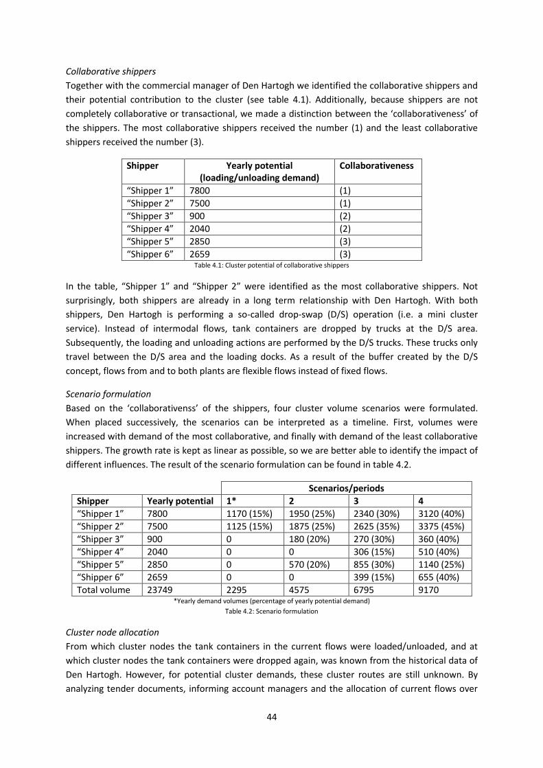
44
Collaborative shippers
Together with the commercial manager of Den Hartogh we identified the collaborative shippers and
their potential contribution to the cluster (see table 4.1). Additionally, because shippers are not
completely collaborative or transactional, we made a distinction between the ‘collaborativeness’ of
the shippers. The most collaborative shippers received the number (1) and the least collaborative
shippers received the number (3).
Shipper Yearly potential (loading/unloading demand)
Collaborativeness
“Shipper 1” 7800 (1)
“Shipper 2” 7500 (1)
“Shipper 3” 900 (2)
“Shipper 4” 2040 (2)
“Shipper 5” 2850 (3)
“Shipper 6” 2659 (3) Table 4.1: Cluster potential of collaborative shippers
In the table, “Shipper 1” and “Shipper 2” were identified as the most collaborative shippers. Not
surprisingly, both shippers are already in a long term relationship with Den Hartogh. With both
shippers, Den Hartogh is performing a so-called drop-swap (D/S) operation (i.e. a mini cluster
service). Instead of intermodal flows, tank containers are dropped by trucks at the D/S area.
Subsequently, the loading and unloading actions are performed by the D/S trucks. These trucks only
travel between the D/S area and the loading docks. As a result of the buffer created by the D/S
concept, flows from and to both plants are flexible flows instead of fixed flows.
Scenario formulation
Based on the ‘collaborativenss’ of the shippers, four cluster volume scenarios were formulated.
When placed successively, the scenarios can be interpreted as a timeline. First, volumes were
increased with demand of the most collaborative, and finally with demand of the least collaborative
shippers. The growth rate is kept as linear as possible, so we are better able to identify the impact of
different influences. The result of the scenario formulation can be found in table 4.2.
Scenarios/periods
Shipper Yearly potential 1* 2 3 4
“Shipper 1” 7800 1170 (15%) 1950 (25%) 2340 (30%) 3120 (40%)
“Shipper 2” 7500 1125 (15%) 1875 (25%) 2625 (35%) 3375 (45%)
“Shipper 3” 900 0 180 (20%) 270 (30%) 360 (40%)
“Shipper 4” 2040 0 0 306 (15%) 510 (40%)
“Shipper 5” 2850 0 570 (20%) 855 (30%) 1140 (25%)
“Shipper 6” 2659 0 0 399 (15%) 655 (40%)
Total volume 23749 2295 4575 6795 9170 *Yearly demand volumes (percentage of yearly potential demand)
Table 4.2: Scenario formulation
Cluster node allocation
From which cluster nodes the tank containers in the current flows were loaded/unloaded, and at
which cluster nodes the tank containers were dropped again, was known from the historical data of
Den Hartogh. However, for potential cluster demands, these cluster routes are still unknown. By
analyzing tender documents, informing account managers and the allocation of current flows over

45
AsIs Scenario 1 Scenario 2 Scenario 3 Scenario 4
Cluster service price €12.85 €12.67 €12.20 €11.97 €11.89
Market price €12.50 €12.50 €12.50 €12.50 €12.50
€11.40
€11.60
€11.80
€12.00
€12.20
€12.40
€12.60
€12.80
€13.00
Pri
ce/h
ou
r
Cluster service rate vs. market rate
terminals, we proposed an allocation of flows from and to the collaborative shippers over terminals
as can be found in Appendix 13. Furthermore, because most tank containers have to be cleaned for
every loading we assumed a cleaning percentage of 80%.
Additional assumptions:
No flows from and to depots are included
In the scenario formulation we do not include potential cluster demands from and to depots.
Flows from cluster nodes to the cleaning station and the other way around are assumed to
be flexible
In the calculation of the scenarios, we assumed the flows from and to the cleaning station are
flexible. Due to variations in waiting and cleaning times, customers will include a time buffer.
Assuming this flow is flexible can therefore be justified.
4.4.2. Scenario results
For every scenario, the cluster service price was calculated and compared with the market price. The
results are presented in figure 4.2. The reader is referred to Appendix 14 for a complete overview of
the results. As showed in figure 4.2, from scenario 2, the cluster service becomes price competitive.
This scenario requires a flexible demand increase of 3825 (59%) tank containers per year and a fixed
demand increase of 750 (28%) tank containers per year. A flexible demand increase of almost 60
percent looks high. However, this increase is based on the positive reactions of “Shipper 1” and
“Shipper 2” on the cluster service.
Figure 4.2: Comparison of the cluster service price with the market price for every demand scenario
# drivers # trucks # chassis # planners
AsIs 15 13 10 2
Scenario 1 17 16 11 2
Scenario 2 20 19 14 2
Scenario 3 23 22 16 2
Scenario 4 25 25 19 2 Table 4.3: Number of resources needed per scenario

46
4.5. Main drivers business case
Volume and matching probabilities were identified as the main potential drivers of the cost savings
per scenario. In this section we analyzed the actual influence of these drivers on the cluster service
price.
Volumes: In the business case, we calculated the cluster service price per hour. We
therefore simply divided the total cluster service costs by the total amount of hours. As a
result, the fixed costs are spread over more hours. Hence, the cost per hour decreases.
However, because the fixed/flexible ratio was different per scenario, the increase in hours
needed to execute the cluster demands were not increased linearly. The growth percentage
compared to the previous scenario is presented in figure 4.3. Additionally, the figure
represents the decline percentage of the cluster service price.
Figure 4.3: Relationship between cluster volumes and cluster price
From observing the figure above, it looks like there is a significant relationship between the
volume and price. An increase in price results in a decrease in costs.
Matching probabilities: In the model, increasing matching probabilities at cluster nodes lead
to lower solo transportation and cluster node times. As mentioned in the detailed
calculation model, matching probabilities are dependent on three factors:
(1) Volumes. Higher volumes result in more matching possibilities and therefore higher
matching probabilities.
(2) The balance between drops and pickups. A balanced number of drops and pickups lead
to lower matching probabilities than an unbalanced number of drops and pickups.
(3) Flexible/fixed ratio. A high flexible/fixed ratio leads to higher matching probabilities.
In the figure below we present the matching probabilities of the six flexible/fixed groups in a
balanced situation (i.e. number of drops equals the number of pickups). The balanced
situation represents the lower bound of the matching probabilities.
0%
5%
10%
15%
20%
25%
30%
1 2 3 4
Ch
ange
co
mp
are
d t
o p
revi
ou
s sc
en
ario
Scenarios
Cluster time vs. cluster price
Total cluster service time
Cluster service price
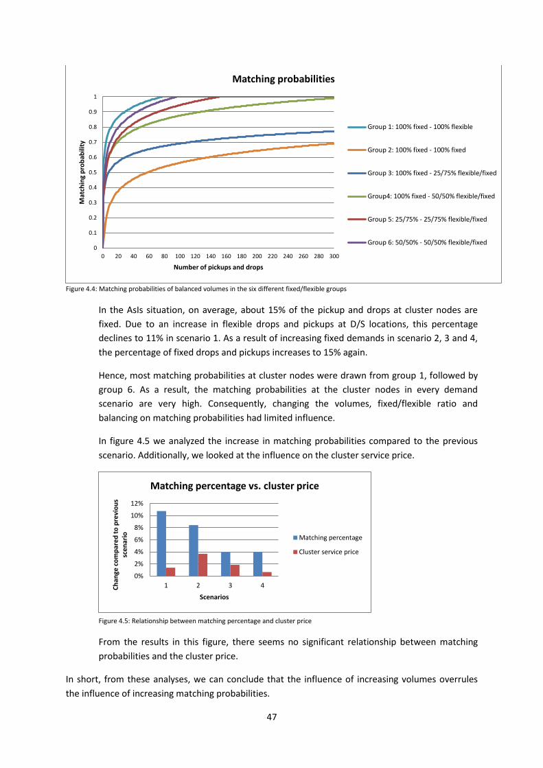
47
Figure 4.4: Matching probabilities of balanced volumes in the six different fixed/flexible groups
In the AsIs situation, on average, about 15% of the pickup and drops at cluster nodes are
fixed. Due to an increase in flexible drops and pickups at D/S locations, this percentage
declines to 11% in scenario 1. As a result of increasing fixed demands in scenario 2, 3 and 4,
the percentage of fixed drops and pickups increases to 15% again.
Hence, most matching probabilities at cluster nodes were drawn from group 1, followed by
group 6. As a result, the matching probabilities at the cluster nodes in every demand
scenario are very high. Consequently, changing the volumes, fixed/flexible ratio and
balancing on matching probabilities had limited influence.
In figure 4.5 we analyzed the increase in matching probabilities compared to the previous
scenario. Additionally, we looked at the influence on the cluster service price.
Figure 4.5: Relationship between matching percentage and cluster price
From the results in this figure, there seems no significant relationship between matching
probabilities and the cluster price.
In short, from these analyses, we can conclude that the influence of increasing volumes overrules
the influence of increasing matching probabilities.
0
0.1
0.2
0.3
0.4
0.5
0.6
0.7
0.8
0.9
1
0 20 40 60 80 100 120 140 160 180 200 220 240 260 280 300
Mat
chin
g p
rob
abili
ty
Number of pickups and drops
Matching probabilities
Group 1: 100% fixed - 100% flexible
Group 2: 100% fixed - 100% fixed
Group 3: 100% fixed - 25/75% flexible/fixed
Group4: 100% fixed - 50/50% flexible/fixed
Group 5: 25/75% - 25/75% flexible/fixed
Group 6: 50/50% - 50/50% flexible/fixed
0%
2%
4%
6%
8%
10%
12%
1 2 3 4Ch
ange
co
mp
are
d t
o p
revi
ou
s sc
en
ario
Scenarios
Matching percentage vs. cluster price
Matching percentage
Cluster service price

48
4.6. Robustness
In this section, we elaborate on the robustness of the business case results. The robustness of the
business case results is checked by challenging the underlying assumptions which could have a
negative impact on the business case.
Strategic assumptions:
Collaborative shippers will always have the same degree of collaborativeness
The collaborative attitude on quality and safety of shippers is critical to the success of the
cluster service. According to the interviewees, this collaborative attitude is part of the
culture of a shipper and will therefore not behave very dynamically. However, changes in the
market will influence the mindset of a shipper in a certain degree. For example, the credit
crisis of 2008 made the shippers focus more on short-term cost advantages, which resulted
in an increase of contracting low cost carriers. However, in the upcoming years, the market
is expected to grow again which may have a positive influence on the collaborativeness of
the shippers.
Initial cluster volumes and fixed/flexible composition remain stable
Although the AsIs situation is determined by the current cluster volumes and their
fixed/flexible composition, if Den Hartogh decides to invest next year or in two years in the
cluster service, these volumes may be changed dramatically. As mentioned several times in
the interviews, the network of a carrier is a ‘living’ creature. Every year, the network changes
due to the tendering of shippers. These changes have also impact on the volumes of the
cluster service. However, the impact is expected to stay with the fixed volumes. Den Hartogh
will always have the need to clean and to store tank containers. As these flexible demands
turned out to be essential to a good cluster service performance, this assumption is defined
as robust.
The market price remains stable
In the different scenarios, we assumed the market price to remain stable. However, when
Den Hartogh introduces the cluster service and starts to take over demand from trucking
operators, the resource utilization of these trucking operators decreases. Consequently,
trucking operators will decrease their prices to fill up this free capacity. The results of the
business case may therefore not be robust to these market forces.
Operational assumptions:
Cluster demands do not overlap with each other
Although we assumed no overlaps between cluster demands, in reality, the overlap
probability is rather big. Due to the fixed loading/unloading moment and their long duration,
fixed demands are expected to overlap when their numbers increase. To determine the
influence of overlapping demands on the cluster service price we performed a small analysis
on the expected maximal amount of overlaps in the AsIs situation and the four different
scenarios. The analysis can be found in Appendix 15. The results are presented in table 4.4.

49
Scenario Price (excluding overlap) Price (including overlap) Difference
AsIs € 12.85 € 12.85 +0.05%
1 € 12.67 € 12.70 +0.28%
2 € 12.20 € 12.22 +0.18%
3 € 11.97 € 11.99 +0.17%
4 € 11.89 € 11.91 +0.18% Table 4.4: Difference between cluster service price including overlap and excluding overlap
From these results, we concluded that overlapping demands do not have a significant impact
on the cluster service price. This conclusion can be explained by the large amount of flexible
demands. Due to the large number of flexible demands, the gaps that are created by fixed
demands can easily be filled. Hence, the utilization of trucks and drivers increases, and the
effect of overlapping demands decreases. In case the number of fixed demands are much
larger, the assumption of ‘no overlapping demands’ cannot be justified anymore.
4.7. Discussion
We finalize this chapter with a discussion on the results of the business case.
Relevance of a 2.8% price disadvantage
As turned out from the calculation of the cluster service price in the AsIs situation, the current price
gap with the market standard is 2.8%. But, how relevant is a gap of ‘just’ 2.8%? On a yearly basis,
this 2.8% represents €11.550 euros of extra costs compared to the outsourcing option. For a
company with an annual turnover of more than 200 million euros, this yearly gap of €11.550 looks
rather small. Hence, the company may decide to compete on price from the start, take the first
losses and focus on the whole market (instead of only collaborative shippers) to create volume.
Although this strategy might seem attractive, the reaction of the market has to be taken into
account. As mentioned in the robustness analysis, trucking companies are likely to react with
decreasing prices as a result of (the potential danger of) increasing resource availability. If the cluster
service decides to focus on the complete market, due to short-term price advantages, transactional
shippers are expected to react first. Consequently, volume is created at transactional shipper
demands, which is subtracted from the volume of trucking operators. In turn, these companies will
react with a lower market price to win back business. In the end, the cluster service has to offer even
lower transportation prices in order to compete with the market. All in all, with a price disadvantage
of 2.8%, a ‘capture-all’ strategy is not expected to be beneficial.
Instead, increasing the volumes at collaborative shippers might create a much more ‘sustained’
competitive advantage. As turned out from the RBV, volumes at collaborative shippers only come
within reach when the carrier is able to create the expectation that long-term benefits (i.e. on
quality and safety) exceed the short-term benefits (i.e. price). However, when a relationship with a
collaborative shipper can be established by the cluster service, it becomes much harder for a
trucking operator to compete. Hence, before focusing on the whole market, it might we more
beneficial to first focus on the demand of collaborative shippers. Due to its long-term characteristic,
the demand of the collaborative shippers creates a stronger foundation to start competing on price
with the trucking operators.

50
Practical influences
Furthermore we identified some practical influences which are not included in the model, but could
have an influence on the results of the business case:
Drivers
As turned out from figure 4.1, driver wages have the highest impact on the cluster service
price. However, these driver costs could be overestimated as a result of the assumption
cluster drivers cannot be used outside the cluster. Because demand is stochastic and the
number of drivers is fixed, drivers can become unutilized. When the cluster service is
integrated with Den Hartogh, these drivers might also be used in the operations of the
company. Consequently, the drivers remain utilized and driver cost decreases.
On the other hand, drivers can become sick or go on vacation. As a result, more drivers have
to be hired than only the number of drivers needed to execute the cluster demands. Driver
wages might therefore be underestimated.
Long-haul transportation
From the cluster demands of Den Hartogh, not every demand is outsourced to trucking
operators. Some cluster flows are used to fill up the gap between two long-distance
transportation jobs. For example, a driver just unloaded his tank container at a chemical
facility and has to perform a next job within 2 hours. Usually, this driver is able to perform a
flexible cluster demand instead of waiting for the next job. As a result, the utilization of this
driver increases. However, when all these cluster demands are performed by the cluster
service, the driver is not able to fill this gap anymore. Hence, the cost of long-haul
transportation drivers and trucks increases. These consequences are not included in the
price gap of 2.8%.
Relevance of fixed/flexible ratio for Den Hartogh
Although the insights of the fixed/flexible ratio are not relevant for the results of this business case,
they might be interested for other operations of Den Hartogh. As turned out from figure 4.4, only a
small number of flexible drops and pickups are necessary to significantly increase the matching
probabilities. Hence, weak spots in the network should be a target for planners, key account
managers and commercial managers to increase the flexible volumes. Flexible volumes may be
created by more flexible customer requirements or local transportation flows (i.e. demands from-
and-to cleanings, terminals or D/S locations).
Another impact of the fixed/flexible ratio insights on the operations of Den Hartogh might be to
reconsider the current cost model. The current cost model charges the customer with a fixed rate on
loading/unloading, pickup/drop, full/empty and solo kilometers, etc. Which may be adjusted a little
bit per region. Consequently, a customer sometimes pays Den Hartogh too much due to high
matching probabilities and sometimes pays Den Hartogh too little due to low matching probabilities.
Hence, there is a lack of visibility and incentive to increase matching probabilities when the rates are
fixed.

51
5. Conclusions & Recommendations In this final chapter, we draw conclusions from our study to the business case of the cluster service
and present our recommendations to Den Hartogh. We first present the conclusions by answering
the research questions from chapter 1. Next, recommendations are formulated based on the
findings of this study.
5.1. Conclusions
1. Is the cluster service able to create a competitive advantage in the chemical cluster of
Rotterdam?
This question needed to be answered for the two phases of the cluster service. The cluster service
has in the first phase a price disadvantage and in the second phase a price advantage.
In the first phase, the cluster service should focus on increasing quality and safety and primarily try
to commit the collaborative shippers. The potential to increase performance on quality and safety
turned out to be mainly dependent on experienced and well-trained cluster drivers. As collaborative
shippers indicated to prefer a cultural and personal match that already has been established with
the provider of the service, the cluster service should be closely connected to name and
performance of Den Hartogh. Because the impact of the threats (i.e. monopoly, opportunistic
behavior and information accessibility) remains low in phase one, the fact Den Hartogh provides the
service will not cause any problems.
In the second phase, besides the collaborative shippers, the cluster service becomes interesting to
the transactional shippers. As the cluster volumes are growing, so are the negative influences of the
threats. To overcome these negative influences, we proposed the cluster service should be
performed by an independent party. Because the cluster service already established a reputation in
the first phase, collaborative shippers will not be deterred.
2. How should the calculation model be designed to calculate the business case of the cluster
service?
A model was designed to determine the total cluster service time to execute the daily demand. The
model consists of three parts: (1) An optimization model that minimizes the time of transportation
within the cluster. As the performance of cluster service is dependent on solo transportation time
and waiting time at cluster nodes, the model tries to match the drop of a tank container with the
pickup of a tank container of two consecutive transportation jobs. (2) To avoid the problem
becoming a VRP, we kept the one-day planning horizon and determined the matching probabilities
of two consecutive transportation demands in a separate model. In this model, we divided the
cluster demands into fixed and flexible demands. Fixed demands are executed on fixed moments of
the day. Flexible demands have more planning freedom. Hence, flexible demands increase the
matching probabilities significantly. In the end, the matching probabilities were used in the
optimization model to capacitate the number of matches. (3) Finally, a simulation program was
designed to approach the stochastic behavior of the demands. 200 demands scenarios were created
and solved by the optimization model.

52
3. What is the business case of the cluster service?
Based on the output of the calculation model, we determined the required number of resources.
Consequently, the cluster service price was calculated and compared with the market price.
In the AsIs situation, the price gap between the cluster service price and the market price turned out
to be 2.8% (i.e. a gap of €11.550 on yearly basis). Based on the findings from the first research
question, we identified the collaborative shippers and determined their potential cluster demand.
Subsequently, we formulated four potential demand scenarios. In the second scenario, with a
flexible demand increase of 3825 tank containers (59%) per year and a fixed demand increase of
750 tank containers (28%) per year, the cluster service reached the critical mass to become price
competitive.
The main driver of this cost decrease turned out to be the increase of volumes. Fixed costs are
allocated over more hours, which resulted in a lower cost per hour. On the other hand, the increase
in matching probabilities appeared to be low. Hence, the impact on the cluster service price was
marginal. The low increase in matching probabilities was explained by the already high matching
probabilities in the AsIs situation. Due to the large number of flexible demands in the cluster,
additional volumes only have a small impact on the probabilities.
5.2. Recommendations
In this section, we discuss the recommendations for implementation of the cluster service. We split
the recommendations into strategic and operational recommendations.
Strategic recommendations
1. Although the gap of 2.8% seems small, the focus should remain on committing collaborative
shippers
As mentioned in the discussion of the business case results, the cluster service does not have
a stable foundation to focus on transactional shippers. Trucking operators are expected to
react on the introduction of the cluster service by offering sharper market prices. As a result,
the gap of 2.8% becomes larger. Instead, when cluster demands are enlarged by volumes of
collaborative shippers, the cluster service will create a more sustained competitive
advantage.
2. Good commercial skills are necessary in the start-up phase of the cluster service
In the start-up phase, the commercial department of Den Hartogh has a large influence on
the success of the cluster service. First of all, collaborative shippers tend to select carriers on
soft organizational criteria. Secondly, the relationship between cause and effect on safety
and quality is harder to quantify. Therefore, the commercial department has to sell safety
and quality more on commitment. Although the collaborative shippers indicated to believe
in the added value of experienced and well-trained drivers, the commitment on safety and
quality can be enlarged by emphasizing the difference between a regular and cluster driver.
For example, by highlighting the different training programs.

53
3. In the start-up phase, the cluster service should focus on the drop-swap operations of
“Shipper 1” and “Shipper 2”
Demand from the D/S operation is perceived as the most favorable demand of the cluster
service. First of all, “Shipper 2” and “Shipper 1” are identified as collaborative shippers.
Secondly, because the demands are not fixed but flexible. This provides a very good
foundation to potential changes in volumes of the cluster service.
4. Introduce a rewarding system
As well as in the current cluster demands as in the four demand scenarios, the demands are
allocated over the same cluster nodes (see Appendix 13). However, when other shippers
become interested in the model, the cluster node allocation may change. If these shipper
make use of cluster nodes with low current volumes and high waiting times (e.g. Uniport),
this could have a significant impact on the matching probabilities. Hence, to increase the
matching probabilities at these cluster nodes, flexible demands have to be introduced. It
might be beneficial to steer customer on their cluster node choice to increase the matching
probabilities.
5.3. Further research
To finalize this chapter, we formulated the following limitations of the study that require further
research.
1. The value of safety and quality
In the RBV model we stated that collaborative shippers are willing to invest in quality and
safety. However, we did not investigate how much shippers are willing to pay extra for these
services. Besides this fee is different among the collaborative shippers, it is very difficult to
quantify the additional value of quality and safety. As mentioned before in this study,
collaborative shippers have to ‘believe’ the additional fee on quality and safety is beneficial
to them on the long term. Hence, the larger the price gap and the lower the quantitative
support, the lower expected willingness of a collaborative shipper to pay the additional fee.
2. Define gain sharing rules
As already mentioned in the final section of the RBV model, gain sharing rules have to be
defined before starting the cluster service. In the start-up phase, only collaborative shippers
are expected to be interested in the cluster service. These shippers have to pay an additional
fee and expect to benefit from the cluster service on the long-term. However, when the
service becomes competitive on price, transactional shippers are not only benefitting from
the lower price, but (in the end) also from a higher quality and safety standards. Because the
collaborative shippers do not have additional benefits from the cluster service compared to
the transactional shippers, this will be perceived as unfair. Hence, from the start, clear and
fair gain sharing rules have to be defined based on the additional fee the shipper has to pay
in the start-up phase.
54
3. Validation
An important limitation of this study is the lack of validation of the calculation model.
Because we designed a model to solve a unique practical problem by integrating several
techniques, the model was not able to be validated.
4. Lack of sequentiality
Another important shortcoming of the model is the lack of sequentiality. We determined the
matching probabilities primarily by the fact demands are fixed or flexible. Hence, a flexible
pickup of a tank container was not restricted by a flexible drop of the same tank container,
or the other way around. Both pickup and drop were used independently by the matching
model to optimize the number of matchings. In short, the flexible pickups and drops are in
fact too flexible. As a result, the calculated matching probabilities are too positive. Further
research, probably on VRP, might be necessary.

55
Written invitation to
tender
•Action taken by shipper:
•A tender procedure always starts with a written invitation by the shipper to tender.
Written reaction on invitation
• Stage 1:
•Action taken by carrier
•The carrier writes a proposal or quotation for a part or all tendered transportation lanes. Additionally, when the RFI is not part of the tender, the carrier writes a commercial text to promote the company and its capabilities. These documents are submitted by the carrier before the formulated deadline.
First selection
•Stage 1:
•Action taken by shipper:
•In the next step, the shipper usually makes a first selection. Furthermore, the selected carriers are provided with feedback on the transportation rates. Normally, the shipper provides a comparison between the transportation rates of the carrier and the lowest rates of the competitors. The feedback can either be communicated by e-mail or at a contact meeting during the second round.
Oral presentatio
n/ negotiation
•Stage 2:
•Action taken by shipper and carrier:
•Based on this feedback, carriers have the opportunity to submit their new proposed rates by e-mail on short term. During the second round, most of the shippers invite the selected carriers for a company presentation and/or a negotiation round.
Second selection
•Stage 3:
•Action taken by shipper:
•Carriers are once again provided with feedback on the transportation rates by e-mail or at a contact meeting during the third round.
Negotiation
•Stage 3:
•Action taken by shipper and carrier:
Final selection
•Action by shipper
•At the third round, as a result of the last negotiation meeting, a final selection was made by the shipper.
Appendix 1: RFP/RFQ procedure

56
Appendix 2: Complaints
Code of cause Name of cause Code of cause Name of cause
002 Customer satisfaction info 049 Equipment breakdown TC's and roadbarrel
011 Human: incorrect behavior 052 Hose rupture
012 Human: customer's instructions not adhered to 061 Wrong equipment planned
013 Human: DH working instruction not adhered to 063 Special equipment missing
016 Human: sudden illness 064 Previous load or cleaning incorrect
022 DH instructions not up-to-date, incorrect or insufficient 071 Non-available: equipment shortage
023 Customer's instructions not up-to-date, incorrect or insufficient 072 Non-available: vehicle delayed on previous assignment
024 Language problem 073 Non-available: drivers shortage
025 EDI or IT issue 091 Traffic/maneuvering accident
031 Documentation incorrect 101 Theft or vandalism
032 Documentation missing 111 Unsafe equipment customer or DH
042 Equipment breakdown chassis 112 Unsafe working environment
043 Equipment breakdown other equipment 134 Traffic violations
045 Equipment incorrect maintenance 151 Traffic delay
046 Equipment breakdown truck 161 Strike
171 Weather conditions
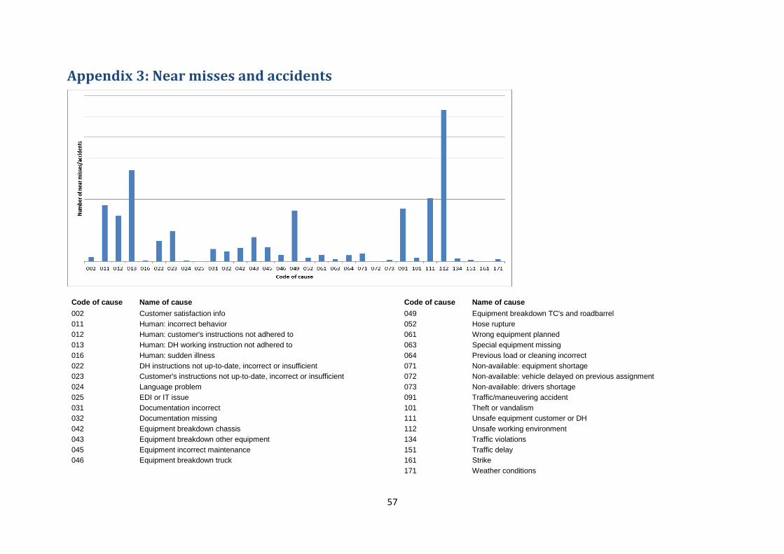
57
Appendix 3: Near misses and accidents
Code of cause Name of cause Code of cause Name of cause
002 Customer satisfaction info 049 Equipment breakdown TC's and roadbarrel
011 Human: incorrect behavior 052 Hose rupture
012 Human: customer's instructions not adhered to 061 Wrong equipment planned
013 Human: DH working instruction not adhered to 063 Special equipment missing
016 Human: sudden illness 064 Previous load or cleaning incorrect
022 DH instructions not up-to-date, incorrect or insufficient 071 Non-available: equipment shortage
023 Customer's instructions not up-to-date, incorrect or insufficient 072 Non-available: vehicle delayed on previous assignment
024 Language problem 073 Non-available: drivers shortage
025 EDI or IT issue 091 Traffic/maneuvering accident
031 Documentation incorrect 101 Theft or vandalism
032 Documentation missing 111 Unsafe equipment customer or DH
042 Equipment breakdown chassis 112 Unsafe working environment
043 Equipment breakdown other equipment 134 Traffic violations
045 Equipment incorrect maintenance 151 Traffic delay
046 Equipment breakdown truck 161 Strike
171 Weather conditions

58
Sh
ipp
er
Ca
rrie
rC
lust
er
serv
ice
Send order to carrier
Book modality at subcontractors
Receive order from shipper
Send order to CS
Receive order from carrier
Send confirmation and book slot at
shipper
Receive confirmation and slot booking from
carrier
Send confirmation to carrier
Receives confirmation from
CS
Provides CS driver with transportation
documents
CS driver receives transportation
documents from shipper
CS driver provides carrier with
transportation documents
Carrier receives transportation
documents from CS
Carrier sends invoice to shipper
CS sends invoice to shipper
Shipper receives invoice from carrier
Shipper receives invoice from carrier
Order process Loading process Invoice process
Appendix 4: Information flow cluster service

59
Loading/unloading at chemical facility
Moving to chemical facility
Waiting at chemical facility
Service at chemical facility
Full/empty transportationSolo
transportation
Pickup tank container at cluster node
Arrival at cluster node
Waiting at cluster node
Container is placed on
chassis
Leaving cluster node
Drop tank container at cluster node
Moving to cluster node
Waiting at cluster node
Remove container from
chassis
Moving to next cluster node
Appendix 5: Typical cluster demand

60
Appendix 6: Cluster nodes and chemical facilities Confidential

61
Appendix 7: Transportation distance In this appendix the distance in time between cluster nodes and chemical facilities is represented. We decided to place the cluster nodes in groups, based
on their location. The average driving distance between adjacent groups is 15 minutes and within a group 7.5 minutes. Two cluster nodes where not able to
place in one of these groups: (1) The chemical plant of “Shipper 3” and (2) the chemical plant of “Shipper 7”. These are treated as exceptions. The grouping
was performed to make adjustments to the number of cluster nodes and chemical plants less time consuming. Furthermore, compared to the plant and
cluster times, transportation time is expected to have a large impact on the performance. Making the distance less exact is therefore not expected to have
significant influences. In the figure the grouping is represented and distance can be found in the table.
From-to (time zones) Shipper 3 BCW Rotterdam Terminal Bontrans Cobelfret DH Cleaning DH ChemiehavenDH Rozenburg De Rijke Botlek DH Trucking Shipper 7 Shipper 6 Shipper 1 DS Shipper 8 Shipper 2 DS P&O RSC RST Noord RST Zuid Uniport Shipper 9 Waalhaven Botlek Terminal Shipper 5 Shipper 4
Shipper 3 0 15 30 30 30 30 30 30 30 30 15 30 15 15 45 15 15 15 15 30 30 30 15
BCW Rotterdam Terminal 15 0 30 30 30 30 30 30 30 45 15 30 15 15 45 7.5 7.5 7.5 7.5 30 30 30 15
Bontrans 30 30 0 7.5 7.5 7.5 7.5 7.5 7.5 60 15 7.5 15 15 15 30 30 30 30 7.5 7.5 7.5 15
Cobelfret 30 30 7.5 0 7.5 7.5 7.5 7.5 7.5 60 15 7.5 15 15 15 30 30 30 30 7.5 7.5 7.5 15
DH Cleaning 30 30 7.5 7.5 0 7.5 7.5 7.5 7.5 60 15 7.5 15 15 15 30 30 30 30 7.5 7.5 7.5 15
DH Chemiehaven 30 30 7.5 7.5 7.5 0 7.5 7.5 7.5 60 15 7.5 15 15 15 30 30 30 30 7.5 7.5 7.5 15
DH Rozenburg 30 30 7.5 7.5 7.5 7.5 0 7.5 0 60 15 7.5 15 15 15 30 30 30 30 7.5 7.5 7.5 15
De Rijke Botlek 30 30 7.5 7.5 7.5 7.5 7.5 0 7.5 60 15 7.5 15 15 15 30 30 30 30 7.5 7.5 7.5 15
DH Trucking 30 30 7.5 7.5 7.5 7.5 0 7.5 0 60 15 7.5 15 15 15 30 30 30 30 7.5 7.5 7.5 15
Shipper 7 30 45 60 60 60 60 60 60 60 0 45 60 45 45 75 45 45 45 45 60 60 60 45
Shipper 6 15 15 15 15 15 15 15 15 15 45 0 15 15 7.5 30 15 15 15 15 15 15 15 7.5
Shipper 1 DS 30 30 7.5 7.5 7.5 7.5 7.5 7.5 7.5 60 15 0 15 15 15 30 30 30 30 7.5 7.5 7.5 15
Shipper 8 15 15 15 15 15 15 15 15 15 45 7.5 15 0 7.5 30 15 15 15 15 15 15 15 7.5
Shipper 2 DS 15 15 15 15 15 15 15 15 15 45 7.5 15 7.5 0 30 15 15 15 15 15 15 15 7.5
P&O 30 45 15 15 15 15 15 15 15 45 30 15 30 30 0 45 45 45 45 15 15 15 30
RSC 15 7.5 30 30 30 30 30 30 30 45 15 30 15 15 45 0 7.5 7.5 7.5 30 30 30 15
RST Noord 15 7.5 30 30 30 30 30 30 30 45 15 30 15 15 45 7.5 0 0 7.5 30 30 30 15
RST Zuid 15 7.5 30 30 30 30 30 30 30 45 15 30 15 15 45 7.5 0 0 7.5 30 30 30 15
Uniport 15 7.5 30 30 30 30 30 30 30 45 15 30 15 15 45 7.5 7.5 7.5 0 30 30 30 15
Shipper 9 30 30 7.5 7.5 7.5 7.5 7.5 7.5 7.5 60 15 7.5 15 15 15 30 30 30 30 0 7.5 7.5 15
Waalhaven Botlek Terminal 30 30 7.5 7.5 7.5 7.5 7.5 7.5 7.5 60 15 7.5 15 15 15 30 30 30 30 7.5 0 7.5 15
Shipper 5 30 30 7.5 7.5 7.5 7.5 7.5 7.5 7.5 60 15 7.5 15 15 15 30 30 30 30 7.5 7.5 0 15
Shipper 4 15 15 15 15 15 15 15 15 15 45 7.5 15 7.5 7.5 30 15 15 15 15 15 15 15 0

62
Chemical facility Waiting + service time (in min)
Shipper 3 199
Shipper 7 120
Shipper 6 280
Shipper 8 240
Shipper 9 60
Shipper 5 112
Shipper 4 191
Appendix 8: Cluster node and chemical facility time In this appendix the waiting + service times of cluster nodes and chemical facilities are represented. Because the data of waiting + service times of cluster
nodes are missing, we base this information on the knowledge of planners of Den Hartogh. Instead, data of waiting + service times of chemical facilities are
based on historical data of Den Hartogh over 2014. We use data of both loading and unloading times, which are assumed to be normal distributed, and
place it in a single distribution. As input value for the model, we use the time which is closest to the 75th percentile of the distribution. This method is also
used by the planning system of Den Hartogh. In this appendix we give an example of this process for one chemical facility.
Example service + waiting times of “Shipper 3”
Cluster nodes Waiting + service times (in min)
BCW Rotterdam Terminal 30
Bontrans 15
Cobelfret 45
DH Cleaning 60
DH Chemiehaven 20
DH Rozenburg 5
De Rijke Botlek 20
DH Trucking 5
Shipper 1 20
Shipper 2 30
P&O 45
RSC 45
RST Noord 75
RST Zuid 75
Uniport 105
Waalhaven Botlek Terminal 30
Chemical facility Average St. dev # loadings Average St. dev # unloadings
Shipper 3 170 132.5236 5 159.504 57.88712 2236
Waiting + service time (in min)
The 75th percentile of the combination of these distributions = 199 minutes

63
From-to BCWROT BONBOT COBROZ DENBOT DENCHE DENROZ DERBOT DHRCHEM Shipper 1 Shipper 2 POEURO RSCROT RSTROT-N RSTROT-Z UNIPROT WAABOT1 pickup (total) drop (total)
BCWROT 0 0 0 0 0 0 0 0 0 0 0 0 0 0 0 0 0 0
BONBOT 0 0 0 0 0 0 0 0 0 0 0 0 0 0 0 0 0 0
COBROZ 0 0 0 1 1 0 0 1 0 0 0 0 0 0 0 0 3 2
DENBOT 0 0 0 5 3 3 4 1 4 0 1 3 0 0 0 0 24 23
DENCHE 0 0 0 1 0 0 2 0 1 0 0 1 0 0 0 0 5 5
DENROZ 0 0 0 1 0 0 0 0 1 0 0 0 0 0 0 0 2 3
DERBOT 0 0 0 1 1 0 0 1 4 0 0 0 0 0 0 0 7 9
DHRCHEM 0 0 0 1 0 0 0 0 0 0 0 0 0 0 0 0 1 4
Shipper 1 0 0 0 5 0 0 3 1 0 0 0 3 0 0 0 0 12 12
Shipper 2 0 0 0 0 0 0 0 0 0 0 0 0 0 0 0 0 0 0
POEURO 0 0 0 0 0 0 0 0 0 0 0 0 0 0 0 0 0 2
RSCROT 0 0 2 0 0 0 0 0 1 0 0 0 0 0 0 0 4 7
RSTROT-N 0 0 0 2 0 0 0 0 0 0 1 0 0 0 0 0 2 0
RSTROT-Z 0 0 0 4 0 0 0 0 0 0 0 0 0 0 0 0 4 0
UNIPROT 0 0 0 2 0 0 0 0 0 0 0 0 0 0 0 0 2 0
WAABOT1 0 0 0 0 0 0 0 0 0 0 0 0 0 0 0 0 1 0
Cluster node Expected # matchings
BCWROT 0
BONBOT 0
COBROZ 2
DENBOT 23
DENCHE 5
DENROZ 2
DERBOT 7
DHRCHEM 1
Shipper 1 12
Shipper 2 0
POEURO 0
RSCROT 4
RSTROT-N 0
RSTROT-Z 0
UNIPROT 0
WAABOT1 0
Appendix 9: Verification of basic model Technique: Tracing
Step 1: We determined the full and empty runs based on an arbitrary demand scenario.
Step 2: The total amount of drops and pickups are presented in the last two columns of the table above. Based on the 100 percent matching assumption,
we expected min(𝑝𝑖𝑐𝑘𝑢𝑝𝑠, 𝑑𝑟𝑜𝑝𝑠) = # 𝑚𝑎𝑡𝑐ℎ𝑖𝑛𝑔𝑠.
Step 3: We verified if number of expected matchings equals the number of calculated matchings by the model

64
From-to BCWROT BONBOT COBROZ DENBOT DENCHE DENROZ DERBOT DHRCHEM Shipper 1 Shipper 2 POEURO RSCROT RSTROT-N RSTROT-Z UNIPROT WAABOT1
BCWROT 0 0 0 0 0 0 0 0 0 0 0 0 0 0 0 0
BONBOT 0 0 0 0 0 0 0 0 0 0 0 0 0 0 0 0
COBROZ 0 0 2 0 0 0 0 0 0 0 0 0 0 0 0 0
DENBOT 0 0 0 23 0 0 0 0 0 0 0 0 0 0 0 0
DENCHE 0 0 0 0 5 0 0 0 0 0 0 0 0 0 0 0
DENROZ 0 0 0 0 0 2 0 0 0 0 0 0 0 0 0 1
DERBOT 0 0 0 0 0 0 7 0 0 0 0 0 0 0 2 0
DHRCHEM 0 0 0 0 0 0 0 1 0 0 0 0 2 1 0 0
Shipper 1 0 0 0 0 0 0 0 0 12 0 0 0 0 0 0 0
Shipper 2 0 0 0 0 0 0 0 0 0 0 0 0 0 0 0 0
POEURO 0 0 1 1 0 0 0 0 0 0 0 0 0 0 0 0
RSCROT 0 0 0 0 0 0 0 0 0 0 0 4 0 3 0 0
RSTROT-N 0 0 0 0 0 0 0 0 0 0 0 0 0 0 0 0
RSTROT-Z 0 0 0 0 0 0 0 0 0 0 0 0 0 0 0 0
UNIPROT 0 0 0 0 0 0 0 0 0 0 0 0 0 0 0 0
WAABOT1 0 0 0 0 0 0 0 0 0 0 0 0 0 0 0 0
Step 4: We verified if the solo transportation time and full/empty transportation time calculated by the model equals the manually calculated times
Manually calculated
o Solo: 210 minutes
o Full/empty: 1365 minutes
Calculated by the model
o Solo 210 minutes
o Full/empty: 1365 minutes
Step 5: We verified if the total cluster node time calculated by the model equals the manually calculated total cluster node time. (Note: As a result of a
match, the waiting time can be neglected). See Appendix 8 for cluster node times.
Manually calculated: 3225 minutes (see table below)

65
Calculated by the model: 3225 minutes
Step 6: We verified if the total plant time calculated by the model equals the manually calculated total plant time
Manually calculated: 2414 minutes (multiplying demand with the waiting + service times at chemical plants in Appendix 8)
Calculated by the model: 2414 minutes
Step 7: We verify if the total cluster service time calculated by the model equals the manually calculated total service time
Manually calculated: 7214 minutes (solo + full/empty + node + chemical facility)
Calculated by the model: 7214 minutes
From-to BCWROT BONBOT COBROZ DENBOT DENCHE DENROZ DERBOT DHRCHEM Shipper 1 Shipper 2 POEURO RSCROT RSTROT-N RSTROT-Z UNIPROT WAABOT1
BCWROT 0 0 0 0 0 0 0 0 0 0 0 0 0 0 0 0
BONBOT 0 0 0 0 0 0 0 0 0 0 0 0 0 0 0 0
COBROZ 0 0 90 0 0 0 0 0 0 0 0 0 0 0 0 0
DENBOT 0 0 0 1380 0 0 0 0 0 0 0 0 0 0 0 0
DENCHE 0 0 0 0 100 0 0 0 0 0 0 0 0 0 0 0
DENROZ 0 0 0 0 0 10 0 0 0 0 0 0 0 0 0 35
DERBOT 0 0 0 0 0 0 140 0 0 0 0 0 0 0 250 0
DHRCHEM 0 0 0 0 0 0 0 5 0 0 0 0 160 80 0 0
Shipper 1 0 0 0 0 0 0 0 0 240 0 0 0 0 0 0 0
Shipper 2 0 0 0 0 0 0 0 0 0 0 0 0 0 0 0 0
POEURO 0 0 90 105 0 0 0 0 0 0 0 0 0 0 0 0
RSCROT 0 0 0 0 0 0 0 0 0 0 0 180 0 360 0 0
RSTROT-N 0 0 0 0 0 0 0 0 0 0 0 0 0 0 0 0
RSTROT-Z 0 0 0 0 0 0 0 0 0 0 0 0 0 0 0 0
UNIPROT 0 0 0 0 0 0 0 0 0 0 0 0 0 0 0 0
WAABOT1 0 0 0 0 0 0 0 0 0 0 0 0 0 0 0 0
Chemical facility Demand
Shipper 3 6
Shipper 7 0
Shipper 6 2
Shipper 8 2
Shipper 9 3
Shipper 5 0
Shipper 4 0

66
Appendix 10: Combining groups of different fixed/flexible ratios Group Drop Pickup Equals Description
1 100% flexible 100% fixed -
2 100% flexible 25% flexible/75% fixed Group 1 When the total amount of drops is flexible, the ratio of pickups is not relevant anymore. Whether a pickup is fixed or flexible, the matching conditions stay the same (i.e. if the drop occurs before the pickup = no match, if the drop occurs after the pickup = match).
3 100% flexible 50% flexible/50% fixed Group 1 See description group 2
4 100% flexible 75% flexible/25% fixed Group 1 See description group 2
5 100% flexible 100% flexible Group 1 See description group 2
6 75% flexible/25% fixed 100% fixed Group 1 The absolute value of the difference between matching probabilities in this group with group 1 were <0.1
7 75% flexible/25% fixed 25% flexible/75% fixed Group 1 See description group 6
8 75% flexible/25% fixed 50% flexible/50% fixed Group 1 See description group 6
9 75% flexible/25% fixed 75% flexible/25% fixed Group 1 See description group 6
10 75% flexible/25% fixed 100% flexible Group 1 Same as group 4
11 50% flexible/50% fixed 100% fixed -
12 50% flexible/50% fixed 25% flexible/75% fixed Group 13 The absolute value of the difference between matching probabilities in this group with group 13 were <0.1
13 50% flexible/50% fixed 50% flexible/50% fixed -
14 50% flexible/50% fixed 75% flexible/25% fixed Group 1 Same as group 8
15 50% flexible/50% fixed 100% flexible Group 1 Same as group 3
16 25% flexible/75% fixed 100% fixed -
17 25% flexible/75% fixed 25% flexible/75% fixed -
18 25% flexible/75% fixed 50% flexible/50% fixed Group 13 The absolute value of the difference between matching probabilities in this group with group 13 were <0.1
19 25% flexible/75% fixed 75% flexible/25% fixed Group 1 Same as group 7
20 25% flexible/75% fixed 100% flexible Group 1 Same as group 2
21 100% fixed 100% fixed -
22 100% fixed 25% flexible/75% fixed Group 16 Same as group 16
23 100% fixed 50% flexible/50% fixed Group 17 Same as group 17
24 100% fixed 75% flexible/25% fixed Group 1 Same as group 6
25 100% fixed 100% flexible Group 1 Same as group 1

67
Lower bound
Simulated
probabilities
1 0.04
2 0.1
3 0.173333333
4 0.1825
5 0.206
6 0.218333333
7 0.23
8 0.24375
9 0.27
10 0.275
11 0.314545455
12 0.33
13 0.310769231
14 0.343571429
15 0.354
16 0.364375
17 0.378235294
18 0.371666667
19 0.377368421
20 0.382
Upper bound
Simulated
probabilities
1 0.04
2 0.12
3 0.2
4 0.17
5 0.24
6 0.28
7 0.3
8 0.34
9 0.42
10 0.42
11 0.4
12 0.44
13 0.5
14 0.4
15 0.43
16 0.43
17 0.43
18 0.59
19 0.54
20 0.45
y = 0.1675ln(x) + 0.0024R² = 0.9012
0
0.1
0.2
0.3
0.4
0.5
0.6
0.7
1 2 3 4 5 6 7 8 9 10 11 12 13 14 15 16 17 18 19 20
Pro
bab
ility
Upper bound (1 drop and # pickups)
Simulated probabilities
Log. (Simulated probabilities)
y = 0.1192ln(x) + 0.021R² = 0.9771
0
0.05
0.1
0.15
0.2
0.25
0.3
0.35
0.4
0.45
1 2 3 4 5 6 7 8 9 10 11 12 13 14 15 16 17 18 19 20
Pro
bab
ility
Lower bound (# drops = # pickups)
Simulated probabilities
Log. (Simulated probabilities)
Appendix 11: Determining matching probabilities In the following steps, we show the process of determining the matching probabilities. We used
Group 2 (100% fixed drops/100% fixed pickups) as example.
Step 1: We simulated the matching probabilities of the upper and lower bound and determined the
logarithmic function.
Step 2: We calculated the maximum number of the lower bound (i.e. up to a matching probability of
0.9). However, as can already be observed from the figure above, the matching probabilities of the
lower bound will never reach 0.9. This can be explained by the fact fixed pickups cannot be matched
in the first hours of the time horizon by the fixed drops. We therefore used a maximum value of 300
drops and pickups. A higher number of drops and pickups is not expected at a cluster node.
Due to the lack of space, we provide the matching probabilities up to 10 drops and pickups in the
table below.

68
Step 3: Finally, we filled up the gaps between upper and lower bound. This is done linearly (see the
table below).
1 2 3 4 5 6 7 8 9 10
1 0.04 0.118502 0.186418 0.234604 0.271981 0.30252 0.32834 0.350706 0.370435 0.388083
2 0.118502 0.109966
3 0.186418 0.156919
4 0.234604 0.190233
5 0.271981 0.216073
6 0.30252 0.237186
7 0.32834 0.255036
8 0.350706 0.270499
9 0.370435 0.284139
10 0.388083 0.296339
# Drops
# Pickups
1 2 3 4 5 6 7 8 9 10
1 0.04 0.118502 0.186418 0.234604 0.271981 0.30252 0.32834 0.350706 0.370435 0.388083
2 0.118502 0.109966 0.316123
3 0.186418 0.156919 0.303905
4 0.234604 0.190233 0.291688
5 0.271981 0.216073 0.279471
6 0.30252 0.237186 0.267254
7 0.32834 0.316123 0.303905 0.291688 0.279471 0.267254 0.255036
8 0.350706 0.270499
9 0.370435 0.284139
10 0.388083 0.296339
# Drops
# Pickups

69
Appendix 12: Cost structure Fixed costs
Confidential
Flexible costs
Confidential

70
Appendix 13: Terminal allocation
Customer Cleaning (%)
Shipper 1 80%
Shipper 2 80%
Shipper 3 80%
Shipper 4 80%
Shipper 5 80%
Shipper 6 80%
Cluster node allocation
Customer BCW Rotterdam Terminal Bontrans Cobelfret DH Cleaning DH Chemiehaven DH Rozenburg De Rijke Botlek DH Trucking Shipper 1 Shipper 2 P&O RSC RST Noord RST Zuid Uniport Waalhaven Botlek Terminal
Shipper 1 18% 12% 40% 1% 28% 1%
Shipper 2 9% 6% 70% 1% 14% 1%
Shipper 3 29% 20% 2% 47% 2%
Shipper 4 22% 15% 25% 1% 35% 2%
Shipper 5 29% 20% 2% 47% 2%
Shipper 6 21% 14% 30% 1% 33% 1%

71
Appendix 14: Scenario result overview
Solo transportation
time (in min)
Empty/full transportation
time (in min) Nodes time (in min) Plant time (in min) Total time (in min) Node visits Plant visits KMs Cluster service rate Market rate
AsIs 334 1330 4115 1912 7691 164.82 11.43 886.75 12.85€ 12.50€
Scenario 1 358 1745 5151 1858 9112 206.36 11.18 1163.64 12.67€ 12.50€
Scenario 2 404 2293 6484 2382 11563 256.20 14.67 1528.98 12.20€ 12.50€
Scenario 3 415 2702 7476 3155 13748 291.05 18.50 1801.18 11.97€ 12.50€
Scenario 4 430 3177 8565 3768 15940 334.92 22.04 2118.10 11.89€ 12.50€
Average results per demand scenario

72
Appendix 15: Cluster demand overlap analysis In the cluster demand overlap analysis we determined the expected maximal amount of overlaps for
every of the 200 different runs in the AsIs situation and the four demand scenarios. We determined
the maximal number instead of the average number, because the expected maximal number of
overlaps will determine the amount of drivers and trucks needed. In the end, we compared the
expected maximal amount of overlaps with the trucks that were needed to execute the demand
sequentially.
At every scenario, the following steps were performed to identify the expected maximal amount of
overlaps (we use the AsIs situation as example):
1. A time horizon and time intervals was introduced
a. AsIs situation: 16 hour time horizon and time intervals of 30 minutes
2. The average duration of a fixed and flexible was determined
a. AsIs situation: 4 hours (8 time intervals) for fixed duration and 1 hour (2 time
intervals) for flexible duration
3. The last possible starting point of a fixed demand was determined
a. AsIs situation: The last starting point was the 25th time interval. The fixed demand
has therefore 25 possible intervals to start.
4. Assuming a uniform distribution, the probabilities a fixed demand could occur at a time
interval was determined
a. AsIs situation:
1st time interval: 1/25
2nd time interval: 2/25 (when a fixed demand starts at the first time interval,
also the second interval is covered)
3rd time interval: 3/25, etc.
8th – 25th time interval: 8/25
26th time interval: 7/25
27th time interval: 6/25, etc.
5. The probabilities were multiplied by the amount of fixed demands to determine the
expected number of fixed demands at every time interval.
a. AsIs situation (1st run):
Fixed demand: 13

73
Time interval
1 2 3 4 5 6 7 8 9 10 11 12 13 14 15 16
Expected demand
0.52 1.04 1.56 2.08 2.6 3.12 3.64 4.16 4.16 4.16 4.16 4.16 4.16 4.16 4.16 4.16
Time interval
17 18 19 20 21 22 23 24 25 26 27 28 29 30 31 32
Expected demand
4.16 4.16 4.16 4.16 4.16 4.16 4.16 4.16 4.16 3.64 3.12 2.6 2.08 1.56 1.04 0.52
6. Next, the flexible demands were included. In this overlap calculation, we assumed the
flexible demands to be completely flexible. These flexible demands will therefore be used to
fill up the gaps at the end and the beginning of the time horizon. If the number of flexible
demands exceeds the number of gaps, the remaining demands are evenly spread over the
time horizon.
a. AsIs situation (1st run):
Flexible demands: 73
The maximum amount of overlaps is determined by:
𝑖𝑓 (𝐹𝑙𝑒𝑥𝑖𝑏𝑙𝑒 𝑑𝑒𝑚𝑎𝑛𝑑 − ∑ 𝐸𝑥𝑝𝑒𝑐𝑡𝑒𝑑 𝑓𝑖𝑥𝑒𝑑 𝑑𝑒𝑚𝑎𝑛𝑑𝑠𝑡) > 0, 𝑡ℎ𝑒𝑛
𝑇
𝑡=1
max (𝐸𝑥𝑝𝑒𝑐𝑡𝑒𝑑 𝑓𝑖𝑥𝑒𝑑 𝑑𝑒𝑚𝑎𝑛𝑑𝑠𝑡) +(𝐹𝑙𝑒𝑥𝑖𝑏𝑙𝑒 𝑑𝑒𝑚𝑎𝑛𝑑∗𝐹𝑙𝑒𝑥𝑖𝑏𝑙𝑒 𝑑𝑢𝑟𝑎𝑡𝑖𝑜𝑛)−(max(𝐸𝑥𝑝𝑒𝑐𝑡𝑒𝑑 𝑓𝑖𝑥𝑒𝑑 𝑑𝑒𝑚𝑎𝑛𝑑𝑠𝑡)∗𝑇𝑖𝑚𝑒 ℎ𝑜𝑟𝑖𝑧𝑜𝑛−∑ 𝐸𝑥𝑝𝑒𝑐𝑡𝑒𝑑 𝑓𝑖𝑥𝑒𝑑 𝑑𝑒𝑚𝑎𝑛𝑑𝑠𝑡)𝑇
𝑡=1
𝑇𝑖𝑚𝑒 ℎ𝑜𝑟𝑖𝑧𝑜𝑛
𝑒𝑙𝑠𝑒
max (𝐸𝑥𝑝𝑒𝑐𝑡𝑒𝑑 𝑓𝑖𝑥𝑒𝑑 𝑑𝑒𝑚𝑎𝑛𝑑𝑡)
Expected maximal number of overlaps:
4.16 +(73 ∗ 2) − (4.16 ∗ 32 − 104)
32= 7.81
7. Finally, the expected maximal number of overlaps is compared with the required amount of
trucks needed to execute the regular cluster demand. If the number of overlaps exceeds the
amount of trucks, additional trucks have to be used
AsIs situation: Regular amount of trucks = 7.92. We therefore do not need additional trucks to
overcome the number of overlaps.

74
Bibliography
Amit, R., & Schoemaker, P. (1993). Strategic assets and organizational rent. Strategic Management Journal, 14(1), 33–46.
Barney, J. (1991). Firm Resources and Sustained Competitive Advantage. Journal of Management, 17(1), 99–120.
Barney, J. (1995). Looking inside for competitive advantage. The Academy of Management Executive, 9(4), 49–61.
Barney, J. (2002). Gaining and sustaining competitive advantage (p. 570). Upper Saddle River, NJ: Prentice Hall.
Bertrand, J. W. M., & Fransoo, J. C. (2002). Operations management research methodologies using quantitative modeling. International Journal of Operations & Production Management, 22(2), 241–264.
Castaneda, J. (2014). Revenue Management Opportunities in the Rotterdam Chemical Port. Erasmus University Rotterdam.
Coates, T. T., & McDermott, C. M. (2002). An exploratory analysis of new competencies: a resource based view perspective. Journal of Operations Management, 20(5), 435–450.
Hoopes, D. G., Madsen, T. L., & Walker, G. (2003). Guest editors’ introduction to the special issue: Why is there a resource-based view? Toward a theory of competitive heterogeneity. Strategic Management Journal, 24(10), 889–902.
Kraaijenbrink, J., Spender, J.-C., & Groen, A. J. (2010). The Resource-Based View: A Review and Assessment of Its Critiques. Journal of Management, 36(1), 349–372.
Law, A. M., & Kelton, W. D. (2000). Simulation modeling and analysis (3rd editio., p. 760). McGraw-Hill.
Lippman, S. A., & Rumelt, R. P. (1982). Uncertain imitability: An analysis of interfirm differences in efficiency under competition. The Bell Journal of Economics, 13(2), 418–438.
Mitroff, I. I., Betz, F., Pondy, L. R., & Sagasti, F. (1974). On managing science in the systems age: Two schemas for the sutudy of science as a whole systems phenomenon. Interfaces, 4(3), 46–58.
Olavarrieta, S., & Ellinger, A. E. (1997). Resource-based theory and strategic logistics research. International Journal of Physical Distribution & Logistics Management, 27(9), 559–587.
Penrose, E. T. (1959). The theory of the growth of the firm (p. 272). Oxford: Blackwell.
Peteraf, M. (1993). The cornerstones of competitive advantage: A resource-based view. Strategic Management Journal, 14(3), 179–191.
Porter, M. E. (1980). Competitive strategy: Techniques for analyzing industries and competitors. New York: Free Press.

75
Porter, M. E. (1981). The contribution of industrial organization to strategic management. The Academy of Management Review, 6(4), 609–620.
Porter, M. E. (1985). Competitive advantage. New York: Free Press.
Porter, M. E. (2007). Clusters and Economic Policy: Aligning Public Policy with the New Economics of Competition [White paper]. Retrieved from http://www.hbs.edu/faculty/Publication Files/Clusters_and_Economic_Policy_White_Paper_8e844243-aa23-449d-a7c1-5ef76c74236f.pdf
Priem, R. L., & Butler, J. E. (2001). Is the resource-based view a useful persective for strategic management research? The Academy of Management Review, 26(1), 22–40.
Rumelt, R. P. (1987). Theory, strategy and entrepreneurship. In D. Teece (Ed.), The competitive challenge. New York, NY: Harper & Row.
Thunnissen, S. K., Van de Bunt, L. G., & Vis, I. F. A. (2015). Sustainable fuels for the transport and maritime sector: A Blueprint of the LNG distribution network. In Bridging the Gap: Theory and Practice in Logistics and Supply Chain Innovation (Zijm, W.H.).
Toni, A. De, & Tonchia, S. (2003). Strategic planning and firms’ competencies: Traditional approaches and new perspectives. International Journal of Operations & Production Management, 23(9), 947–976.
Van Aken, J. E. (1994). De bedrijfskunde als ontwerpwetenschap: De regulatieve en de reflective cyclus. Tijdschrift voor Modern Management, 66(1), 16–26.
Van Aken, J. E. (2004). Management Research Based on the Paradigm of the Design Sciences: The Quest for Field-Tested and Grounded Technological Rules. Journal of Management Studies, 41(2), 219–246.
Van de Bunt, L. G. (2014). Literature review: Resource-based view in Logistic Alliances. Eindhoven University of Technology.
Vasconcellos, J. A., & Hambrick, D. C. (1989). Key success factors: Test of a general framework in the mature industrial-product sector. Strategic Management Journal, 10(4), 453–458.
Wernerfelt, B. (1984). A resource-based view of the firm. Strategic Management Journal, 5(2), 171–180.
Woodside, A. (2010). Case Study Research: Theory, Methods and Practice (1st editio., p. 455). Emerald Group Publishing Limited.