grupo de investigación de mecánica de fluidos … · ∗grupo de investigación de mecánica de...

CFD & OPTIMIZATION 2011 - 000

An ECCOMAS Thematic Conference

23-25 May 2011, Antalya TURKEY

AERODYNAMIC OPTIMIZATION OF HIGH-SPEED TRAINS NOSE

USING A GENETIC ALGORITHM AND ARTIFICIAL NEURAL

NETWORKS

J. Muñoz-Paniagua∗, J. García∗ and A. Crespo∗

∗Grupo de Investigación de Mecánica de Fluidos apicada a la Ingeniería IndustrialEscuela Técnica Superior de Ingenieros Industriales, Universidad Politécnica de Madrid

C/ José Gutiérrez Abascal 2, 28006, Madrid, Spaine-mail: [email protected]

Key words: Shape Optimization, High-speed train, Genetic Algorithm, Metamodel,Arti�cial Neural Network, Bèzier Curves

Abstract. An aerodynamic optimization of the train aerodynamic characteristics in termof front wind action sensitivity is carried out in this paper. In particular, a genetic algo-rithm (GA) is used to perform a shape optimization study of a high-speed train nose. Thenose is parametrically de�ned via Bèzier Curves, including a wider range of geometriesin the design space as possible optimal solutions. Using a GA, the main disadvantage todeal with is the large number of evaluations need before �nding such optimal. Here it isproposed the use of metamodels to replace Navier-Stokes solver. Among all the posibili-ties Response Surface Models and Arti�cial Neural Networks (ANN) are considered. Bestresults of prediction and generalization are obtained with ANN and those are applied inGA code. The paper shows the feasibility of using GA in combination with ANN for thisproblem, and solutions achieved are included.

1

J. Muñoz-Paniagua, J. García and A. Crespo

1 INTRODUCTION

The increasing importance of trains as an alternative means of transport, which alsocomplements reducing the tra�c of an already overwhelmed communications network,justi�es the need to carry out studies related to improve its performance. Even when thetrain makes the most economical use of energy form of public transport, reducing energyconsumption is pretended. Consumption is directly related to its aerodynamic. Then, itis necessary to perform aerodynamic studies of the train in order to improve its e�ciency.The aim of the research is the de�nition of optimal nose shapes which involve a minimaldrag coe�cient. This is traditionally done by a trial-and-error procedure, but it is veryexpensive in terms of machine and designer time, and rely heavily on previous analyses.Instead, an automatic method of optimization of aerodynamic shapes is proposed here.This method involves the use of genetic algorithms (GA) as the optimization tool1.

GA are a technique that mimic the mechanics of natural evolution. Once a popula-tion of potential solutions is de�ned, it combines survival-of-the-�ttest concept to elimi-nate un�t characteristics and utilizes random information exchange, with exploitation ofknowledge contained in old solutions, to e�ect a search mechanism with power and speed2.Iteratively, better results are obtained until a solution closer to globally optimal solutionis reached. However, the main drawback when using GA is their need of a large numberof evaluations of the objective function. Furthermore, this problem is considerably moreimportant when evaluations are computational cost-e�ective.

To remedy this inconvenience, the use of metamodels is proposed here. The basic ideaof metamodels is to construct approximations of the analysis codes or numerical solversthat are more e�cient to run, enabling a faster evaluation and optimization process.Metamodeling involves choosing an experimental design for generating data, choosing amodel to represent the data, and then �tting the model to the observed data. ResponseSurface Models3 (RSM) and Kriging models4 have been already applied as metamodels inhigh-speed train optimization. In this paper, a comparative study of RSM and Arti�cialNeural Networks is performed.

2 OPTIMIZATION METHODS

As it has been indicated, the objective is to geometrically optimize the nose of a high-speed train by minimizing its drag coe�cient when it is exposed to a frontal wind. Thissingle-objective optimization problem can be de�ned by5

Minimize f(~x)

subject to gj(~x) ≤ 0 j = 1...m (1)

hl(~x) = 0 l = 1...n

xli ≤ xi ≤ xu

i i = 1...k

being ~x the vector of design variables and f(~x) the objective function. The optimaldesign minimize this function. The inequality and equality constraints represent respec-

2


tively constraints to be satis�ed by the optimal candidate and relations between its designvariables. The di�erent optimization methods existing are classi�ed depending on the or-der of derivatives of the objective function used. Zero-order methods, such as randomsearch, simulated annealing and evolutionary algorithms (among which GA are included)use only the function values in their search for the minimum, while �rst and second ordermethods use respectively the �rst and second derivatives, commonly known as gradientmethods and Newton method. Although the latter are more precise, they require somegradient information of the objective function, which can be a numerically intensive task,especially if the number of design variables is large and if one single evaluation is nu-merically expensive5. Moreover, the reliability and success of gradient methods generallyrequires a smooth design space and the existence of only a single global extremum, or aninitial guess close enough to the global extremum that will ensure proper convergence6.Since in the �eld of aerodynamics, objective functions often have multi-peaks7, it is ex-pected that non-gradient methods will work more e�ciently. Then, for a multimodal andhigh-dimensional design space GA are proposed as optimization method.

2.1 Genetic Algorithm

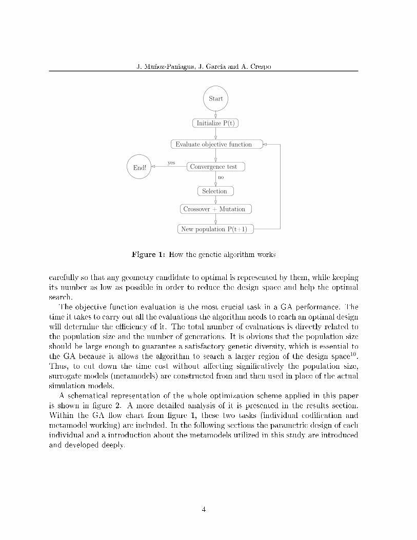
A GA is a stochastic optimization method based on darwinian natural evolution. Itrepeatedly modi�es a set of individuals (population) considered as optimal candidatesby means of three operators, selection, crossover and mutation. At each iteration thealgorithm selects individuals at random from the current population to be parents, anduse them to produce the children for the next generation. Although such operation worksrandomly it is driven in such a way that bene�cts the selection of those individuals whoresult in the �ttest candidates. Children are produced either by making random changesto a single parent (mutation operator) or by combining a couple of parents (crossover).There are a large number of di�erent de�nitions of each operator1. Both operations areperformed with an speci�c probability, mutation probability Pm and crossover probabilityPc respectively. Once new individuals are obtained, the algorithm replaces the currentpopulation with the children to form the next generation, and the population size remainsconstant. The optimal values is always searched for within a group of possible solutions,which is an important di�erence from other one-by-one basis search methods. Figure 1shows schematically how the GA works. In order to stop the iterative process, a conver-gence test according to a pre�xed stopping criteria is done after every new population isevaluated. If this is satis�ed, it ends the cycle. Otherwise, it continues until convergenceis observed.

Each individual is de�ned as a codi�ed structure. The most common way to representeach one is by binary code, so an individual is a bit string. This string is created byconcatenating a number of genes, being each one the codi�cation of each design variable.Therefore, it is necessary to represent each possible optimal design (i.e. a high-speed trainnose shape) as a design vector. The design vector consists out of parameters that de�nethe shape of the geometry. These parameters, and their respective range, must be chosen

3


Evaluate objective function

Initialize P(t)

Convergence test

Selection

Crossover + Mutation

New population P(t+1)

Start

End!yes

no

Figure 1: How the genetic algorithm works

carefully so that any geometry candidate to optimal is represented by them, while keepingits number as low as possible in order to reduce the design space and help the optimalsearch.

The objective function evaluation is the most crucial task in a GA performance. Thetime it takes to carry out all the evaluations the algorithm needs to reach an optimal designwill determine the e�ciency of it. The total number of evaluations is directly related tothe population size and the number of generations. It is obvious that the population sizeshould be large enough to guarantee a satisfactory genetic diversity, which is essential tothe GA because it allows the algorithm to search a larger region of the design space10.Thus, to cut down the time cost without a�ecting signi�catively the population size,surrogate models (metamodels) are constructed from and then used in place of the actualsimulation models.

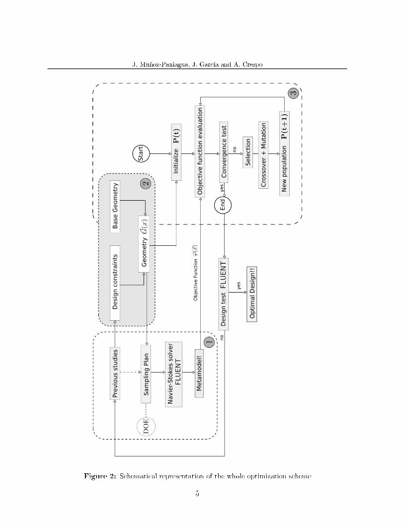
A schematical representation of the whole optimization scheme applied in this paperis shown in �gure 2. A more detailed analysis of it is presented in the results section.Within the GA �ow chart from �gure 1, these two tasks (individual codi�cation andmetamodel working) are included. In the following sections the parametric design of eachindividual and a introduction about the metamodels utilized in this study are introducedand developed deeply.

4


Figure 2: Schematical representation of the whole optimization scheme

5


3 OPTIMIZATION APPROACH

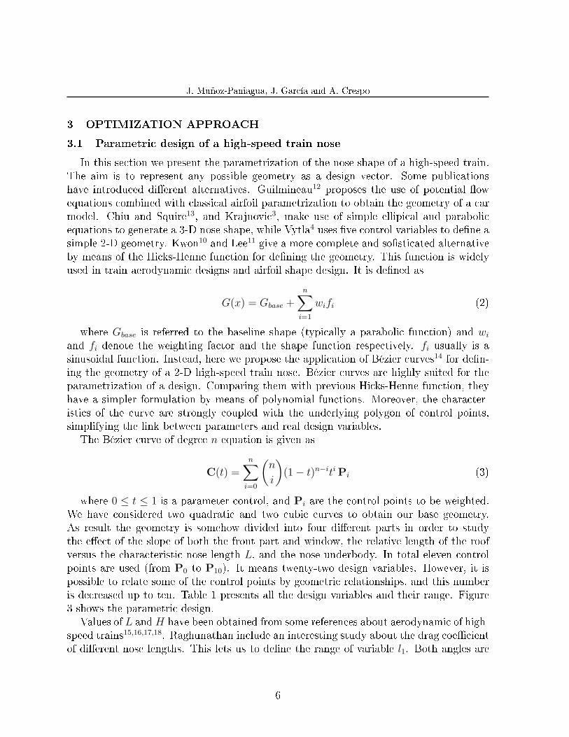
3.1 Parametric design of a high-speed train nose

In this section we present the parametrization of the nose shape of a high-speed train.The aim is to represent any possible geometry as a design vector. Some publicationshave introduced di�erent alternatives. Guilmineau12 proposes the use of potential �owequations combined with classical airfoil parametrization to obtain the geometry of a carmodel. Chiu and Squire13, and Krajnovic3, make use of simple ellipical and parabolicequations to generate a 3-D nose shape, while Vytla4 uses �ve control variables to de�ne asimple 2-D geometry. Kwon10 and Lee11 give a more complete and so�sticated alternativeby means of the Hicks-Henne function for de�ning the geometry. This function is widelyused in train aerodynamic designs and airfoil shape design. It is de�ned as

G(x) = Gbase +n∑

i=1

wifi (2)

where Gbase is referred to the baseline shape (typically a parabolic function) and wi

and fi denote the weighting factor and the shape function respectively. fi usually is asinusoidal function. Instead, here we propose the application of Bézier curves14 for de�n-ing the geometry of a 2-D high-speed train nose. Bézier curves are highly suited for theparametrization of a design. Comparing them with previous Hicks-Henne function, theyhave a simpler formulation by means of polynomial functions. Moreover, the character-istics of the curve are strongly coupled with the underlying polygon of control points,simplifying the link between parameters and real design variables.

The Bézier curve of degree n equation is given as

C(t) =n∑

i=0

(n

i

)(1 − t)n−iti Pi (3)

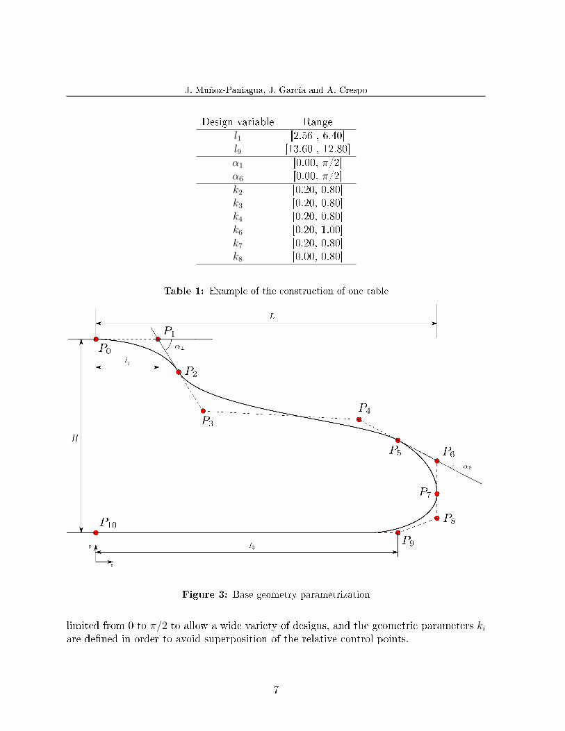
where 0 ≤ t ≤ 1 is a parameter control, and Pi are the control points to be weighted.We have considered two quadratic and two cubic curves to obtain our base geometry.As result the geometry is somehow divided into four di�erent parts in order to studythe e�ect of the slope of both the front part and window, the relative length of the roofversus the characteristic nose length L, and the nose underbody. In total eleven controlpoints are used (from P0 to P10). It means twenty-two design variables. However, it ispossible to relate some of the control points by geometric relationships, and this numberis decreased up to ten. Table 1 presents all the design variables and their range. Figure3 shows the parametric design.

Values of L and H have been obtained from some references about aerodynamic of high-speed trains15,16,17,18. Raghunathan include an interesting study about the drag coe�cientof di�erent nose lengths. This lets us to de�ne the range of variable l1. Both angles are

6


Design variable Rangel1 [2.56 , 6.40]l9 [13.60 , 12.80]α1 [0.00, π/2]α6 [0.00, π/2]k2 [0.20, 0.80]k3 [0.20, 0.80]k4 [0.20, 0.80]k6 [0.20, 1.00]k7 [0.20, 0.80]k8 [0.00, 0.80]

Table 1: Example of the construction of one table

Figure 3: Base geometry parametrization

limited from 0 to π/2 to allow a wide variety of designs, and the geometric parameters ki

are de�ned in order to avoid superposition of the relative control points.

7


3.2 Metamodels. Response Surface Model and Arti�cial Neural Network

The expensive cost of running complex engineering simulations makes it impracticalto rely exclusively on numerical codes for the purpose of aerodynamic optimization. Al-though it is possible to perform all the evaluations on a processors cluster18 for a simpli�edgeometry, it still results in a too long process. By using approximation models, we re-place the expensive simulation model and speed up the genetic algorithm performance.A variety of metamodelling techniques exist, and an excelent comparison and review ofthese methods can be found in some references19,20. Jin20 points out that there is no bestone, although some works better than others for a speci�c application. To compare themaccuracy, e�ciency, robustness, model transparency and simplicity must be taken intoaccount. Therefore, the simplest one, Response Surface Model, is compared in this paperwith Arti�cial Neural Networks, which is a well-considered technique for large-scale prob-lems (ten or more design variables) and low-order nonlinearity (square regression around0.99 when using �rst or second-order polynomial model).

The classical polynomial response surface model (RSM) is still probably the mostwidely used form of surrogate model in engineering design. A second-order polynomialmodel can be expressed as

y(~x) = ϕ(~x) = β0 +k∑

i=1

βixi +k∑

i=1

βiix2i +

∑i

∑j

βijxixj (4)

The coe�cients β are determined by least squares regression analysis by �tting theresponse surface approximations ϕ(~x) to already evaluated designs y(~x). A more completediscussion of RSM is found in Myers22. The main drawback is that for a second-orderpolynomial, the number of unknowns (coe�cients) is proportional to (k + 1)(k + 2)/2,so it is clear that it is not the best method to apply when a high-dimensional design spaceis considered.

An arti�cial neural network (ANN) is composed of many very simple processing units(neurons) connected to form a network. Each connection is characterized by the corre-sponding weight, which speci�es the e�ect of each unit on the overall model. Amongall di�erent types of neural networks, multi-layer percepton (MLP) is considered in thispaper. In an MLP, the network is arranged in layers of processing units: an input layer,one or more hidden layers, and an output one. In our ANN the input layer, composed ofas many input units as dimensions of the design space, is connected to the unique hiddenlayer with nh hidden neurons, which �nally is connected to the output layer of just oneoutput unit. Then, the approximation function is given as

ϕ(~x) =

nh∑j=1

wojzj(~x) + bo

j (5)

where woj is the weight given to the connection of the j-th hidden neuron and the

8


output unit, boj the error or bias associated to the j-th hidden neuron and zj(~x) is the base

function. While in the case of polynomial models this function is pre�xed, in ANN zj(~x)is de�ned as

zj(~x) = g(k∑

i=0

whijxi) (6)

being whij the intensity of the connection between the i-th unit of the input layer and

the j-th one in the hidden layer. Function g(·) is known as the activation function. A widevariety of activation functions exists. Here sigmoidal function is applied. It is expressedas g(a) = 1

1+e−a . The composition of both functions gives the relation between inputs andoutputs for a ANN.

ϕ(~x) =

nh∑j=0

wojg

(k∑

i=0

whijxi

)(7)

Consequently, the unknowns to be adjusted are the connection weights woj and wh

ij,and the number of hidden neurons nh. The determination of the unknown parametersis called the training of the ANN. Back-propagation is the most commonly used methodfor training of multilayer networks. It is a form of supervised learning method. Thedesired output for a given set of input (Ntrn) is known during training. The error at eachneuron is calculated as the di�erence btween the approximated solution and the desiredoutput. This error is then asigned to each of the hidden neurons according to the outputvalues of each hidden neuron and its relative connecting weight. In order to minimize sucherror, the connecting weights are modi�ed and corrected. Training process continues untiltraining error is minimal. However, sometimes the network is able to learn the trainingdata, and laterly it is unable to predict new unobserved data. To avoid it, another set ofdata, Nval is considered to compute the validation error and to indicate if over�tting isobserved while training process is running. Finally, a third set of data is used to checkthe prediction capability of the metamodel once the training has �nished. In this way, theexisting or evaluated designs to �t the metamodel have to be divided into three di�erentsubsets.

4 RESULTS

Metamodel building involves choosing an `experimental' design for generating a databaseand �tting the model to the observed data. The accuracy of the approximation predic-tions depends on the information contained in the database. To maximize this informationand �t the model by a representative sample of the design space Design of Experiments(DOE) method is applied. Traditionally, experimental designs like factorial or fractionalfactorial designs, developed for e�ective physical experiments, have been used. However,because of the deterministic nature of the response, no random error exists in a computer

9


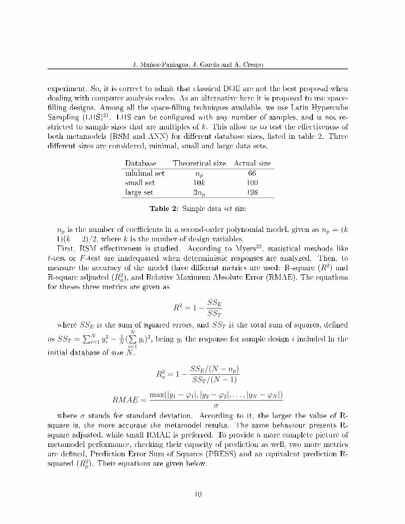
experiment. So, it is correct to admit that classical DOE are not the best proposal whendealing with computer analysis codes. As an alternative here it is proposed to use space-�lling designs. Among all the space-�lling techniques available, we use Latin HypercubeSampling (LHS)21. LHS can be con�gured with any number of samples, and is not re-stricted to sample sizes that are multiples of k. This allow us to test the e�ectiveness ofboth metamodels (RSM and ANN) for di�erent database sizes, listed in table 2. Threedi�erent sizes are considered, minimal, small and large data sets.

Database Theoretical size Actual sizeminimal set np 66small set 10k 100large set 3np 198

Table 2: Sample data set size

np is the number of coe�cients in a second-order polynomial model, given as np = (k+ 1)(k + 2)/2, where k is the number of design variables.

First, RSM e�ectiveness is studied. According to Myers22, statistical methods liket-test or F -test are inadequated when deterministic responses are analyzed. Then, tomeasure the accuracy of the model three di�erent metrics are used: R-square (R2) andR-square adjusted (R2

a), and Relative Maximum Absolute Error (RMAE). The equationsfor theses three metrics are given as

R2 = 1 − SSE

SST

where SSE is the sum of squared errors, and SST is the total sum of squares, de�ned

as SST =∑N

i=1 y2i − 1

N(

N∑i=1

yi)2, being yi the response for sample design i included in the

initial database of size N .

R2a = 1 − SSE/(N − np)

SST /(N − 1)

RMAE =max(|y1 − ϕ1|, |y2 − ϕ2|, . . . , |yN − ϕN |)

σ

where σ stands for standard deviation. According to it, the larger the value of R-square is, the more accurate the metamodel results. The same behaviour presents R-square adjusted, while small RMAE is preferred. To provide a more complete picture ofmetamodel performance, checking their capacity of prediction as well, two more metricsare de�ned, Prediction Error Sum of Squares (PRESS) and an equivalent prediction R-squared (R2

p). Their equations are given below.

10


PRESS =N∑

i=1

(yi − ϕ(i))2

R2p = 1 − PRESS

SST

(8)

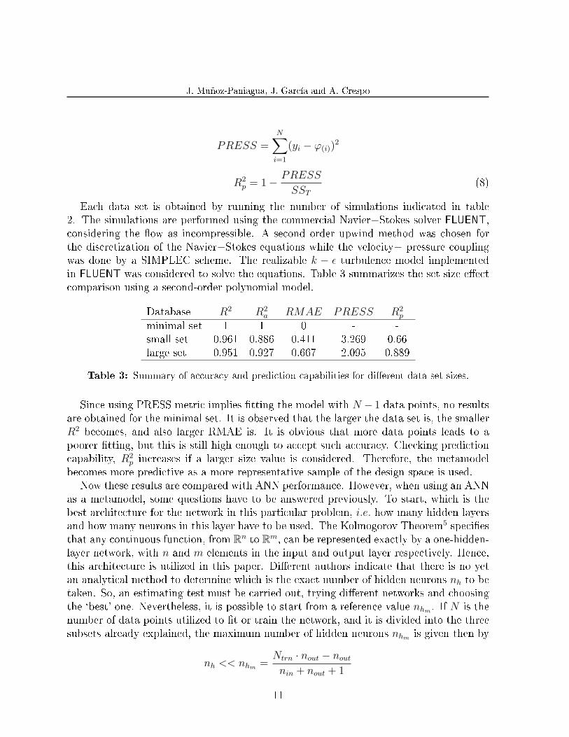
Each data set is obtained by running the number of simulations indicated in table2. The simulations are performed using the commercial Navier−Stokes solver FLUENT,considering the �ow as incompressible. A second order upwind method was chosen forthe discretization of the Navier−Stokes equations while the velocity− pressure couplingwas done by a SIMPLEC scheme. The realizable k − ε turbulence model implementedin FLUENT was considered to solve the equations. Table 3 summarizes the set size e�ectcomparison using a second-order polynomial model.

Database R2 R2a RMAE PRESS R2

p

minimal set 1 1 0 - -small set 0.961 0.886 0.411 3.269 0.66large set 0.951 0.927 0.667 2.095 0.889

Table 3: Summary of accuracy and prediction capabilities for di�erent data set sizes.

Since using PRESS metric implies �tting the model with N − 1 data points, no resultsare obtained for the minimal set. It is observed that the larger the data set is, the smallerR2 becomes, and also larger RMAE is. It is obvious that more data points leads to apoorer �tting, but this is still high enough to accept such accuracy. Checking predictioncapability, R2

p increases if a larger size value is considered. Therefore, the metamodelbecomes more predictive as a more representative sample of the design space is used.

Now these results are compared with ANN performance. However, when using an ANNas a metamodel, some questions have to be answered previously. To start, which is thebest architecture for the network in this particular problem, i.e. how many hidden layersand how many neurons in this layer have to be used. The Kolmogorov Theorem5 speci�esthat any continuous function, from Rn to Rm, can be represented exactly by a one-hidden-layer network, with n and m elements in the input and output layer respectively. Hence,this architecture is utilized in this paper. Di�erent authors indicate that there is no yetan analytical method to determine which is the exact number of hidden neurons nh to betaken. So, an estimating test must be carried out, trying di�erent networks and choosingthe `best' one. Nevertheless, it is possible to start from a reference value nhm . If N is thenumber of data points utilized to �t or train the network, and it is divided into the threesubsets already explained, the maximum number of hidden neurons nhm is given then by

nh << nhm =Ntrn · nout − nout

nin + nout + 1

11


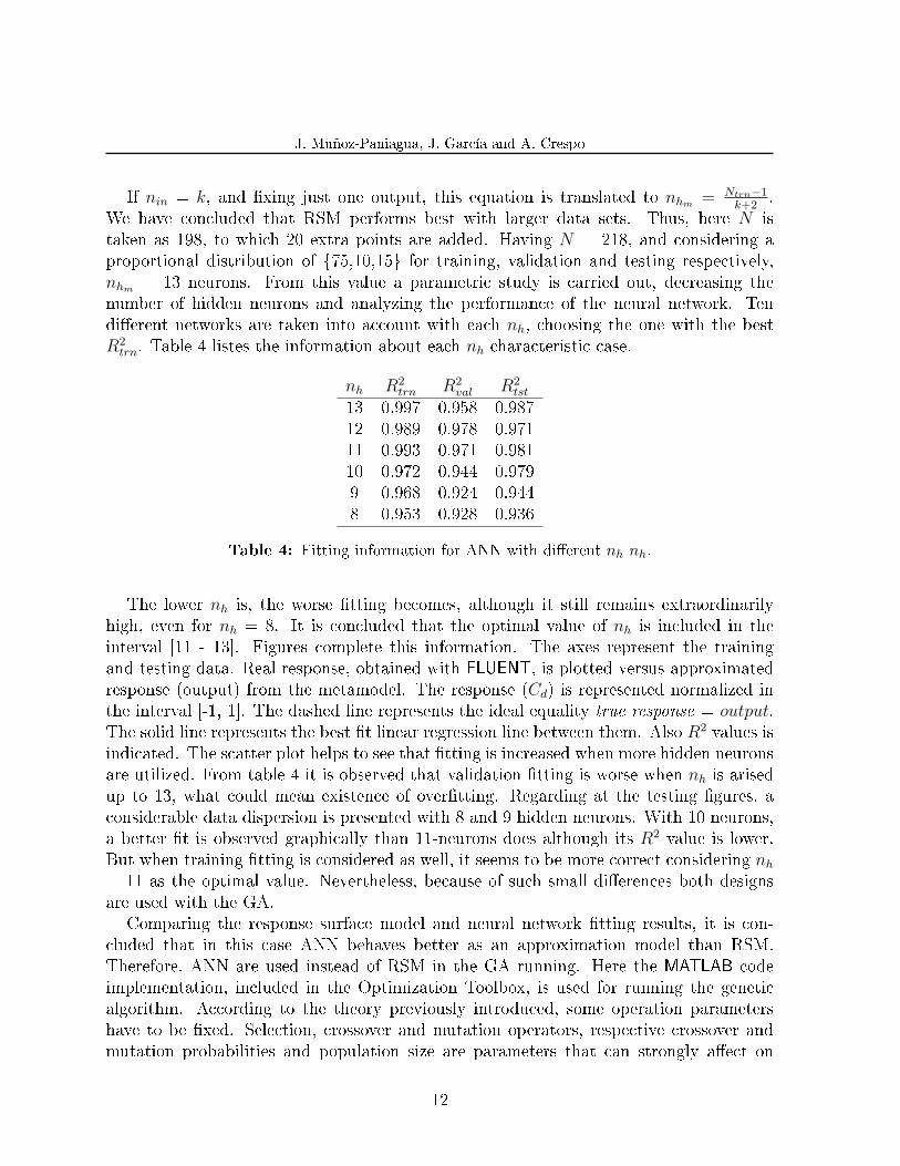
If nin = k, and �xing just one output, this equation is translated to nhm = Ntrn−1k+2

.We have concluded that RSM performs best with larger data sets. Thus, here N istaken as 198, to which 20 extra points are added. Having N = 218, and considering aproportional distribution of {75,10,15} for training, validation and testing respectively,nhm = 13 neurons. From this value a parametric study is carried out, decreasing thenumber of hidden neurons and analyzing the performance of the neural network. Tendi�erent networks are taken into account with each nh, choosing the one with the bestR2

trn. Table 4 listes the information about each nh characteristic case.

nh R2trn R2

val R2tst

13 0.997 0.958 0.98712 0.989 0.978 0.97111 0.993 0.971 0.98110 0.972 0.944 0.9799 0.968 0.924 0.9448 0.953 0.928 0.936

Table 4: Fitting information for ANN with di�erent nh nh.

The lower nh is, the worse �tting becomes, although it still remains extraordinarilyhigh, even for nh = 8. It is concluded that the optimal value of nh is included in theinterval [11 - 13]. Figures complete this information. The axes represent the trainingand testing data. Real response, obtained with FLUENT, is plotted versus approximatedresponse (output) from the metamodel. The response (Cd) is represented normalized inthe interval [-1, 1]. The dashed line represents the ideal equality true response = output.The solid line represents the best �t linear regression line between them. Also R2 values isindicated. The scatter plot helps to see that �tting is increased when more hidden neuronsare utilized. From table 4 it is observed that validation �tting is worse when nh is arisedup to 13, what could mean existence of over�tting. Regarding at the testing �gures, aconsiderable data dispersion is presented with 8 and 9 hidden neurons. With 10 neurons,a better �t is observed graphically than 11-neurons does although its R2 value is lower.But when training �tting is considered as well, it seems to be more correct considering nh

= 11 as the optimal value. Nevertheless, because of such small di�erences both designsare used with the GA.

Comparing the response surface model and neural network �tting results, it is con-cluded that in this case ANN behaves better as an approximation model than RSM.Therefore, ANN are used instead of RSM in the GA running. Here the MATLAB codeimplementation, included in the Optimization Toolbox, is used for running the geneticalgorithm. According to the theory previously introduced, some operation parametershave to be �xed. Selection, crossover and mutation operators, respective crossover andmutation probabilities and population size are parameters that can strongly a�ect on

12


(a) nh = 8 (b) nh = 9

(c) nh = 10 (d) nh = 11

(e) nh = 12 (f) nh = 13

Figure 4: Training regression plots for neural networks considered in table 4.13


(a) nh = 8 (b) nh = 9

(c) nh = 10 (d) nh = 11

(e) nh = 12 (f) nh = 13

Figure 5: Testing regression plots for neural networks considered in table 4.14


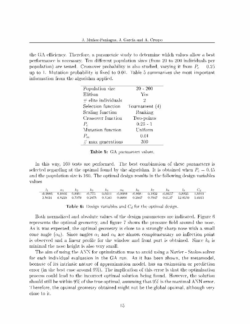
the GA e�ciency. Therefore, a parametric study to determine which values allow a bestperformance is necessary. Ten di�erent population sizes (from 20 to 200 individuals perpopulation) are tested. Crossover probability is also studied, varying it from Pc = 0.25up to 1. Mutation probability is �xed to 0.01. Table 5 summarizes the most importantinformation from the algorithm applied.

Population size 20 - 200Elitism Yes# elite individuals 2Selection function Tournament (4)Scaling function RankingCrossover function Two-pointsPc 0.25 - 1Mutation function UniformPm 0.01# max generations 300

Table 5: GA parameters values.

In this way, 160 tests are performed. The best combination of these parameters isselected regarding at the optimal found by the algorithm. It is obtained when Pc = 0.45and the population size is 160. The optimal design results in the following design variablesvalues

l1 α1 k2 k3 k4 α6 k6 k7 k8 l9 Cd

-0.9993 0.0466 0.9901 -0.7751 0.0611 -0.9989 -0.9981 0.1822 -0.9657 0.8025 1.0013

2.5614 0.8229 0.7970 0.2675 0.5183 0.0009 0.2047 0.5547 0.0137 12.6159 1.0013

Table 6: Design variables and Cd for the optimal design.

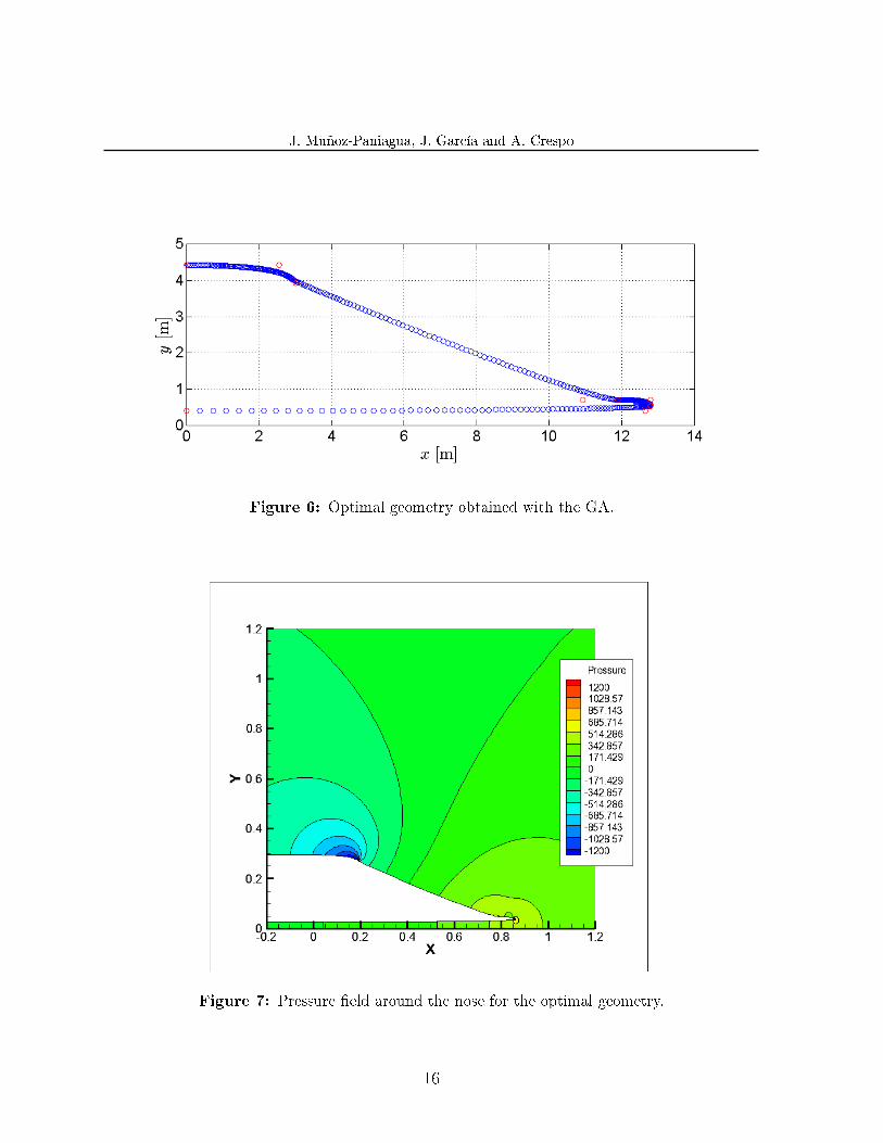
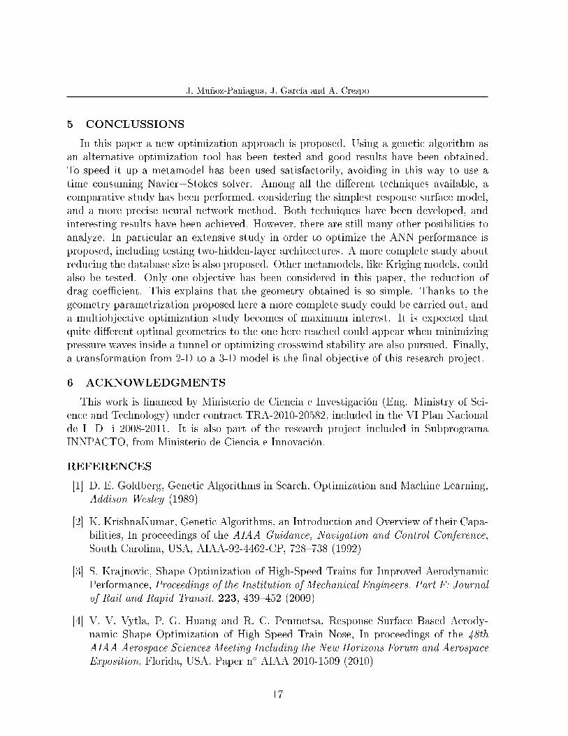
Both normalized and absolute values of the design parameters are indicated. Figure 6represents the optimal geometry, and �gure 7 shows the pressure �eld around the nose.As it was expected, the optimal geometry is close to a strongly sharp nose with a smallcone angle (α6). Since angles α1 and α6 are almost complementary no in�ection pointis observed and a linear pro�le for the window and front part is obtained. Since k6 isminimal the nose height is also very small.

The aim of using the ANN for optimization was to avoid using a Navier - Stokes solverfor each individual evaluation in the GA run. As it has been shown, the metamodel,because of its intrinsic nature of approximation model, has an estimation or predictionerror (in the best case around 9%). The implication of this error is that the optimizationprocess could lead to the incorrect optimal solution being found. However, the solutionshould still be within 9% of the true optimal, assuming that 9% is the maximal ANN error.Therefore, the optimal geometry obtained might not be the global optimal, although veryclose to it.

15


Figure 6: Optimal geometry obtained with the GA.

Figure 7: Pressure �eld around the nose for the optimal geometry.

16


5 CONCLUSSIONS

In this paper a new optimization approach is proposed. Using a genetic algorithm asan alternative optimization tool has been tested and good results have been obtained.To speed it up a metamodel has been used satisfactorily, avoiding in this way to use atime consuming Navier−Stokes solver. Among all the di�erent techniques available, acomparative study has been performed, considering the simplest response surface model,and a more precise neural network method. Both techniques have been developed, andinteresting results have been achieved. However, there are still many other posibilities toanalyze. In particular an extensive study in order to optimize the ANN performance isproposed, including testing two-hidden-layer architectures. A more complete study aboutreducing the database size is also proposed. Other metamodels, like Kriging models, couldalso be tested. Only one objective has been considered in this paper, the reduction ofdrag coe�cient. This explains that the geometry obtained is so simple. Thanks to thegeometry parametrization proposed here a more complete study could be carried out, anda multiobjective optimization study becomes of maximum interest. It is expected thatquite di�erent optimal geometries to the one here reached could appear when minimizingpressure waves inside a tunnel or optimizing crosswind stability are also pursued. Finally,a transformation from 2-D to a 3-D model is the �nal objective of this research project.

6 ACKNOWLEDGMENTS

This work is �nanced by Ministerio de Ciencia e Investigación (Eng. Ministry of Sci-ence and Technology) under contract TRA-2010-20582, included in the VI Plan Nacionalde I+D+i 2008-2011. It is also part of the research project included in SubprogramaINNPACTO, from Ministerio de Ciencia e Innovación.

REFERENCES

[1] D. E. Goldberg, Genetic Algorithms in Search, Optimization and Machine Learning,Addison Wesley (1989)

[2] K. KrishnaKumar, Genetic Algorithms, an Introduction and Overview of their Capa-bilities, In proceedings of the AIAA Guidance, Navigation and Control Conference,South Carolina, USA, AIAA-92-4462-CP, 728�738 (1992)

[3] S. Krajnovic, Shape Optimization of High-Speed Trains for Improved AerodynamicPerformance, Proceedings of the Institution of Mechanical Engineers. Part F: Journalof Rail and Rapid Transit, 223, 439�452 (2009)

[4] V. V. Vytla, P. G. Huang and R. C. Penmetsa, Response Surface Based Aerody-namic Shape Optimization of High Speed Train Nose, In proceedings of the 48thAIAA Aerospace Sciences Meeting Including the New Horizons Forum and AerospaceExposition, Florida, USA, Paper n◦ AIAA 2010-1509 (2010)

17


[5] T. Verstraete, Multidisciplinary Turbomachinery Component Optimization Consid-ering Performance, Stress and Internal Heat Transfer, Ph.D Thesis, Universiteit Gent,Belgium (2008)

[6] T. L. Holst and T. H. Pulliam, Aerodynamic Shape Optimization using a Real-number-encoded Genetic Algorithm, In proceedings of the 19th AIAA Applied Aero-dynamics Conference, California, USA, Paper n◦ A01-31030 (2001)

[7] M. Suzuki, M. Ikeda and K. Yoshida, Study on Numerical Optimization of Cross-sectional Panhead Shape for High-Speed Train, Journal of Mechanical Systems forTransportation and Logistics, 1 100�110 (2008)

[8] J. J. Grefenstette, Optimization of Control Parameters for Genetic Algorithms, IEEETransactions on Systems, Man and Cybernetics, 16, 122�128 (1986)

[9] Genetic Algorithm and Direct Search ToolboxTM 2, User's Guide, MATLAB (2008)

[10] H.-B. Kwon, K.-H. Jang, Y.-S. Kim, K.-Y. Yee and D.-H. Lee, Nose Shape Opti-mization of High-Speed Train for Minimization of Tunnel Sonic Boom, JSME Inter-national Journal Series C, 44, 890�899 (2001)

[11] J. Lee and J. Kim, Approximate Optimization of High-Speed Train Nose Shape forReducing Micropressure Wave, Structural Multidiscipline Optimization, 35, 79�87(2008)

[12] E. Guilmineau and F. Chometon, E�ect of Side Wind on a Simpli�ed Car Model.Experimental and Numerical Analysis, Journal of Fluids Engineering, 131 (2009)

[13] T. W. Chiu and L. C. Squire, An Experimental Study of the Flow over a Trainin a Crosswind at large Yaw Angles up to 90◦, Journal of Wind Engineering andIndustrial Aerodynamics, 45, 47�74 (1992)

[14] G. Farin, Curves and Surfaces for Computer-Aided Geometric Design. A PracticalGuide, Academic Press Professional, 3rd ed. (1993)

[15] F. Cheli, F. Ripamonti, D. Rocchi and G. Tomasini, Aerodynamic behaviour inves-tigation of the new EMUV250 train to cross wind, Journal of Wind Engineering andIndustrial Aerodynamics, 98, 189�201 (2010)

[16] R. S. Raghunathan, H.-D. Kim and T. Setoguchi, Aerodynamics of High-Speed Rail-way Train, Progress in Aerospace Sciences, 38, 469�514 (2002)

[17] J. A. Schetz, Aerodynamics of High-Speed Trains, Annual Review of Fluid Mechanics,33, 371�414 (2001)

18


[18] J. B. Doyle, R. J. Hart�eld and C. Roy, Aerodynamic optimization for freight trucksusing a genetic algorithm and CFD, In proceedings of the 48th AIAA AerospaceSciences Meeting and Exhibit, Nevada, USA, Paper n◦ AIAA 2008-323 (2008)

[19] A. A. Giunta, S. F. Wojtkiewicz Jr. and M. S. Eldred, Overview of modern designof experiments methods for computational simulations, In proceedings of the 41stAIAA Meeting, Nevada, USA, Paper n◦ AIAA 2003-649 (2003)

[20] R. Jin, W. Chen and T. W. Simpson, Comparative studies of metamodelling tech-niques under multiple modelling criteria, Journal of Structure and MultidisciplinaryOptimization, 23, 1�13 (2001)

[21] T. W. Simpson and J. D. Peplinski, Metamodels for computer-based engineering de-sign. Survey and recommendations, Engineering with Computers,17, 129�150 (2001)

[22] R. H. Myers and A. I. Khuri and W. H. C. Jr., Response Surface Methodology.1966−1988, Technometrics 31 137�157 (1989)

19

grupo de investigación de mecánica de fluidos … · ∗grupo de investigación de mecánica de...

Documents