journal of comparative economics - hongliang zhang of comparative economics 45 (2017) 246–260 ......

Journal of Comparative Economics 45 (2017) 246–260

Contents lists available at ScienceDirect

Journal of Comparative Economics

journal homepage: www.elsevier.com/locate/jce

Does population control lead to better child quality? Evidence

from China’s one-child policy enforcement �

Bingjing Li a , Hongliang Zhang

b , ∗

a Department of Economics, National University of Singapore, 1 Arts Link, 117570, Singapore b Department of Economics, Hong Kong Baptist University, Hong Kong

a r t i c l e i n f o

Article history:

Available online 20 September 2016

JEL Classification:

J13

I2

O1

Keywords:

Quantity-quality trade-off

Family planning

Child education

a b s t r a c t

Li, Bingjing , and Zhang, Hongliang —Does population control lead to better child quality?

Evidence from China’s one-child policy enforcement

Scholarly evidence on the quantity-quality trade-off is mixed in part because of the identi-

fication challenge due to endogenous family size. This paper provides new evidence of the

causal effect of child quantity on child quality by exploiting regional differences in the en-

forcement intensity of China’s one-child policy (OCP) as an exogenous source of variation

in family size. Using the percentage of current mothers of primary childbearing age who

gave a higher order birth in 1981, we construct a quantitative indicator of the extent of lo-

cal violation of the OCP, referred to as the excess fertility rate (EFR). We then use regional

differences in EFRs, net differences in pre-existing fertility preferences and socio-economic

characteristics, to proxy for regional differences in OCP enforcement intensity. Using micro

data from the Chinese Population Censuses, we find that prefectures with stricter enforce-

ment of the OCP have experienced larger declines in family size and also greater improve-

ments in children’s education. Despite the evident trade-off between family size and child

quality in China, our quantitative estimates suggest that China’s OCP makes only a modest

contribution to the development of its human capital. Journal of Comparative Economics 45

(2017) 246–260. Department of Economics, National University of Singapore, 1 Arts Link,

117570, Singapore; Department of Economics, Hong Kong Baptist University, Hong Kong.

© 2016 Association for Comparative Economic Studies. Published by Elsevier Inc. All rights

reserved.

1. Introduction

The relationship between child quantity and child quality has long been questioned in social science and public policy.

Beginning with the seminal work by Gary Becker and his associates ( Becker, 1960; Becker and Lewis, 1973; Becker and

Tomes, 1976 ), economists have developed a rich theoretical framework to understand the interaction between child quan-

tity and child quality by seeing both as utility-maximizing choices of households (see, e.g., Hazan and Berdugo (2002) ;

Moav (2005) . A direct implication of this framework is a trade-off between quantity and quality: an exogenous reduction

� We thank Jungmin Lee, Pak Wai Liu, Wallace Mok, Mark Rosenzweig, Junsen Zhang, and four anonymous referees for their helpful comments and

suggestions. Hongliang Zhang acknowledges financial support from the Natural Science Foundation of China (No. 71403233 ). All remaining errors are ours. ∗ Corresponding author.

E-mail addresses: [email protected] (B. Li), [email protected] (H. Zhang).

http://dx.doi.org/10.1016/j.jce.2016.09.004

0147-5967/© 2016 Association for Comparative Economic Studies. Published by Elsevier Inc. All rights reserved.


http://www.ScienceDirect.com

http://www.elsevier.com/locate/jce

http://crossmark.crossref.org/dialog/?doi=10.1016/j.jce.2016.09.004&domain=pdf

http://dx.doi.org/10.13039/501100001809

mailto:[email protected]

mailto:[email protected]


B. Li, H. Zhang / Journal of Comparative Economics 45 (2017) 246–260 247

in family size increases parental investment per child and therefore improves child quality. Although a negative quantity-

quality relationship has been widely observed (for surveys, see King (1987) ; Blake (1989) ), the cross-sectional association

cannot be interpreted as the causal effect of quantity on quality because of the endogeneity issues plaguing this relationship.

First, child quantity and child quality are simultaneously determined parental choices, and both are affected by unobserved

parental heterogeneity. Second, not only can family size affect child quality, but child quality can also affect family size. For

both sources of endogeneity, the effect on the observed quantity-quality relationship is a priori ambiguous. 1

To tackle the endogeneity problems, the literature exploits plausibly exogenous variation in family size caused by either

the natural occurrence of twin births or the sibling sex composition, but yields mixed results. For example, on the one

hand, an adverse effect of family size on children’s outcomes is evidenced by Rosenzweig and Wolpin (1980) for India, by

Stafford (1987) and Cáeres-Delpiano (2006) for the US, by Lee (2008) for South Korea, and by Millimet and Wang (2011) for

Indonesia. On the other hand, Black et al. (2005) , Angrist et al. (2010) , and Fitzsimons and Malde (2014) find no causal link

between child quantity and child quality in Norway, Israel, and Mexico, respectively.

The Chinese context attracts the most scholarly attention in the empirical quantity-quality trade-off literature because of

the availability of high-quality twins’ data and the country’s distinct family planning policy. Using twinning among siblings

as an instrument for the family size of non-twin children, Li et al. (2008) find that twinning increases the family size

and decreases the education of non-twin siblings. Also exploiting twinning as an exogenous variation in family size but

examining the human capital outcomes of both twins and non-twins, Rosenzweig and Zhang (2009) find that both the own

and cross-sib effects of twinning are negative and demonstrate that they yield, respectively, the upper and lower bounds

on the quantity-quality trade-off. Although China’s national family planning policy is often referred to as the “one-child

policy” (OCP), additional births are not always strictly prohibited, and there exist substantial geographical variations in OCP

enforcement. In two previous studies, Qian (2009) and Liu (2014) both exploit differences in local statutory fertility control

policies as exogenous variations for family size to test the quantity-quality trade-off in China, but yield contradictory results.

Making use of regional differences in relaxation rules that allow rural couples to have a second child if the first child is a

girl, Qian (2009) finds that an additional child increases school enrollment of firstborn girls. In contrast, using regional

differences in eligibility criteria for having two children and fines on unsanctioned births, Liu (2014) finds that family size

exerts an adverse effect on child quality when measured by child height.

An important difference between the current paper and prior research is that we use a de facto measure of local OCP

enforcement intensity that takes into account not only the harshness of local statutory fertility policy, as is the studies

of both Qian (2009) and Liu (2014) , but also the stringency of policy compliance in practice. We construct a quantitative

indicator of the extent of local violation of the OCP using the percentage of current Han mothers (i.e., women with at

least one surviving child) of primary childbearing age who gave a higher order birth in 1981. This quantitative indicator,

which we refer to as the “excess fertility rate” (EFR), is analogous to the general fertility rate in definition, except that

both the numerator and denominator are restricted to current mothers. We then measure geographical variations in OCP

enforcement intensity based on the differences in EFRs across localities, net differences in pre-existing fertility preferences

and socio-economic characteristics. Note that this measurement of program intensity follows the spirit of Duflo (2001) , who

gauges regional differences in the intensity of Indonesia’s school construction program in the 1970s by differences in the

number of schools constructed, net differences in the number of children of primary school age.

Using the 1% sample of the 1982 and 1990 Chinese Population Censuses, we find that prefectures with stricter enforce-

ment of the OCP experienced larger declines in family size, but also greater improvements in child education. Under the

assumption that there are no omitted time-varying, region-specific determinants of children’s education that are correlated

with local OCP enforcement intensity, we use the interaction between local OCP enforcement intensity and census year as

the instrument to estimate the causal effect of family size on the education of firstborn children aged 14–17. Our instrumen-

tal variable (IV) estimates show that having an additional sibling decreases the education level by 0.12 for boys and 0.07 for

girls. When junior secondary school attendance is used as the outcome measure, our estimates indicate that an additional

sibling lowers the probability of attending junior secondary school by 13.3 and 11.1 percentage points for boys and girls,

respectively.

Using local OCP enforcement intensity as an instrument for family size to identify the quantity-quality trade-off is not

without potential problems. First, OCP enforcement intensity may be correlated with unobserved concurrent region-specific

shocks to children’s education, such as local school provision and enforcement of nine-year universal education. To address

this potential concern, we further investigate the relationship between the EFR and education of children in the 1990 census

by mother’s age. We find a significant negative relationship only for children whose mother is aged 45 or below in 1990

(i.e., aged 35 or below when the OCP was enacted in 1980), but no apparent relationship for children whose mother is aged

46 or above in 1990 (i.e., aged above 36 or above in 1980). That the EFR is not associated with the education of children of

older mothers whose fertility was barely affected by the OCP is evidence suggesting that our IV estimates of the quantity-

quality trade-off are not confounded by a spurious correlation between the EFR and improvement in child education across

regions.

1 First, omitted parental heterogeneity can result in a spurious (positive or negative) correlation between family size and child education if parental

preferences for child quantity and child quality are correlated with each other. Second, owing to two competing mechanisms with opposite effects, the

overall effect of child quality on family size is also ambiguous. A higher quality child raises parental expectation of the quality of subsequent births, which

may increase fertility. However, a higher quality child also decreases the marginal utility of an additional birth, which may decrease fertility.

248 B. Li, H. Zhang / Journal of Comparative Economics 45 (2017) 246–260

Second, the stringency of local OCP enforcement may affect the education of firstborn children through channels other

than family size. For example, Ebenstein (2010) , Li et al. (2011) , and Chen et al. (2013) all find that stricter fertility control

policy induces a more male-biased sex ratio in China. 2 Although the own sexes of children in our analysis sample are not

affected by OCP enforcement as all of these children were born before the launch of the OCP, the sexes of their younger sib-

lings (if any) are affected. To the extent that sibling sex can affect a child’s education, the validity of using OCP enforcement

intensity as an instrument for family size is challenged when differences in the stringency of local OCP enforcement also

lead to different sibling sex compositions. Similar to Ebenstein (2010) , we find that in our sample stricter OCP enforcement

leads to a more distorted sex ratio at higher parity births only if the first child is a daughter. Thus, our IV estimates for

firstborn boys are not confounded by the omission of the channel of sibling sex composition. Moreover, we argue that if

for girls a male sibling generates a larger negative effect than a female sibling, as is likely to be the case in the Chinese

context, our IV estimates for girls are biased upward. This may explain our estimates of a smaller adverse family size effect

for girls than boys. By comparing the difference in the school enrollment of firstborn girls and firstborn boys in regions

allowing a second birth if a first child is a girl to that in regions without such a relaxation, Qian (2009) finds that having

an additional child has a positive effect on the schooling of firstborn girls. As we demonstrate in this paper, compared with

their counterparts in more strict regions, firstborn girls in less strict regions are exposed to both a larger sibling size and a

less distorted sibling sex selection, the latter of which is beneficial to their human capital investment. Omitting the second

force leads to an upward biased estimate of the quantity-quality trade-off for girls, which may explain the positive estimate

of the family size effect on the relative school enrollment of girls compared with boys in the study by Qian (2009) .

The remainder of this paper is organized as follows. Section 2 introduces the background of China’s family planning pol-

icy and the geographic variations in its enforcement. Section 3 describes the data and illustrates the identification strategy in

a difference-in-differences framework. Section 4 presents the estimated effects of OCP enforcement intensity on family size

and child education. Section 5 uses OCP enforcement intensity as an instrument to estimate the effect of family size on child

education. Section 6 investigates the heterogeneous effects of family size on agricultural and non-agricultural households.

Section 7 discusses the potential bias that may arise from sibling sex selection and measurement error. Section 8 concludes

the paper.

2. Local OCP enforcement

After three decades of rapid population growth, China enacted the OCP as a national policy in 1979 to curb its population

explosion and promote economic growth. In the 1980s, except for Xinjiang and Tibet, the two provincial-level autonomous

regions with the most lenient fertility control, the remaining 28 provincial-level divisions adopted provincial family plan-

ning regulations, setting explicit exemption rules for the issuance of permits for a second child (and under very rare cir-

cumstances a third child). These provincial-level family planning regulations generally do not allow urbanites to have a

second child, but vary in their exemption rules for rural couples to have a second child. 3 Based on these exemption rules

and provincial population composition, Gu et al. (2007) summarize the stringency of provincial-level fertility control poli-

cies using a policy fertility rate calculated as the weighted average birth quota per family, which ranges from 1.06 to 2.37.

Scharping (2003) compiles the provincial-level fine rates imposed on unsanctioned births, which also vary substantially.

Although the national and provincial policies provide the basis for implementing the OCP, there exists a wide variation

in local enforcement when the national and provincial policies are carried out by local governments adapting to local con-

ditions. Differences in local enforcement come from two sources. First, local governments at the prefecture or county level

have drawn up particular regulations that account for the local economic conditions, population density, arable land per

capita, fertility preference, etc. 4 For example, using community survey data from the China Health and Nutrition Survey

(CHNS), Qian (2009) and Liu (2014) both illustrate that even within the same province, there are substantial variations in

local statutory fertility regulations. Second, localities with similar statutory fertility regulations also differ in their extent of

compliance with these regulations because of differences in administrative capacities, implementation methods, work styles,

etc. However, local differences in the enforcement intensity of statutory fertility regulations are largely ignored in the litera-

ture because of data shortages and measurement challenges. An exception is Poston and Gu (1987) , who measure the extent

of OCP compliance at the province level using the percentage share of first parity births among all births and refer to it as

the “first-birth rate”.

In contrast to the first-birth rate used in Poston and Gu (1987) , the EFR constructed in the current paper reflects instead

the extent of local violation of the OCP. Using the 1982 Census microdata, we calculate the EFR as the percentage of current

2 In a similar cultural context, Lin et al. (2014) also find that access to sex-selective abortion increases the male-biased sex ratio in Taiwan, although no

fertility control policy is enforced there. 3 Feng and Hao (1992) summarize the provincial-level family planning regulations of these 28 provinces and classify them into three categories according

to their exemption rules for issuing permits for a second child for rural couples: (i) a strict 1-child policy in five provinces that do not allow rural couples

to have a second child (Beijing, Jiangsu, Shanghai, Sichuan, and Tianjin); (ii) a 1.5-child policy in 18 provinces that allow rural couples to have a second

child if the first child is a girl; and (iii) a 2-child policy in five provinces that authorize rural couples to have two children (Guangdong, Hainan, Ningxia,

Qinghai, and Yunnan). 4 For a more detailed discussion, see Greenhalgh (1986) .


Han mothers aged 25–44 who gave a higher order birth in 1981. 5 Appendix A provides the formula and a detailed discussion

for calculating the EFR. EFR should be 0 if the OCP is strictly enforced with no exception. A positive EFR reflects imperfect

compliance with the OCP, with a larger value corresponding to more relaxed enforcement. Among the prefectures in our

sample, the median EFR is 6.8%, suggesting that compliance with the OCP is far from perfect. There is also a wide variation

in EFR across prefectures, with the standard deviation and interquartile range equaling 4.5% and 5.6%, respectively.

3. Data and identification strategy

3.1. Data

The data used in this paper are taken from the 1% sample of the 1982 and 1990 Chinese Population Censuses. The

census microdata contain information about each individual’s age, sex, region of residence, education, and relationship to

the household head. Because there are no questions in the census that directly link parents to children, we can infer the

parent-child relationship only if the parents are labeled as “head” or “spouse” and the children are labeled as “child” in the

relationship identifier. We thus restrict our sample to households consisting of a “head,” a “spouse,” and at least one “child.”

For women aged 15–64, the censuses asked their number of births and number of surviving children. To get an accurate

account of family size and birth order, we further restrict our sample to households for which the number of children

still staying in the household (i.e., the number of individuals labeled as “child”) equals the number of surviving children

reported by the female head (i.e., the female individual labeled as “head” or “spouse”). For concern over measurement error,

we exclude households for which the age gap between the female head and the eldest child is less than 15. Moreover, we

exclude households with multiple births, as twinning may affect the outcomes of both twins and non-twins ( Rosenzweig

and Zhang, 2009 ). Finally, we exclude households from Xinjiang and Tibet, which have very different OCP enforcement and

economic conditions than the rest of China.

In our analysis of family size and education, the child sample is restricted to firstborn Han children aged 14–17 in the two

censuses. Note that although China adopted its Compulsory Schooling Law in 1986, setting the target for nine-year universal

education, the law tailored the deadlines to attain the target under local conditions and required only the most developed

areas (covering approximately 25% of the country’s population) to achieve nine-year universal education by 1990. 6 Thus, the

quantity-quality trade-off (if any) is likely to be most discernible among those children of secondary school age. Moreover,

we restrict to children below the age of 18 because adult children who have left their parents’ houses are not observed in

the sample.

Our final sample consists of 88,897 households from the 1982 Census and 147,103 households from the 1990 Census.

Table 1 provides summary statistics of the two census samples, both for all children (Columns 1 and 2) and for boys

(Columns 3 and 4) and girls (Columns 5 and 6) separately. There is no significant distinction between the two census

samples in terms of the age and sex of firstborn children. The average number of children per household decreased from

3.59 in 1982 to 2.60 in 1990. This decline is largely attributable to the sharp drop in the proportion of families with four

or more children, from more than half in 1982 to less than one sixth in 1990. The census uses an ordered discrete variable

education level to indicate the highest level of education attained: 1 for illiterate or semi-illiterate, 2 for primary school, 3

for junior secondary school, and 4 for senior secondary school or above. 7 , 8 The average education level of firstborn children

aged 14–17 increased only slightly from 2.64 in 1982 to 2.70 in 1990, and the rise was entirely due to educational improve-

ment of girls (from 2.51 to 2.63). The distribution of children’s education level became less dispersed from 1982 to 1990,

with shifts from both the bottom (i.e., illiterate/semi-literate) and top (i.e., senior middle school) categories to the middle

two categories (i.e., primary school and junior middle school).

3.2. Identification strategy

In this subsection, we illustrate our identification strategy in a difference-in-differences framework. The family size of the

1990 sample (i.e., children born in 1973 and 1976) was subject to much greater influence of the OCP than the 1982 sample

(i.e., children born in 1965 and 1968) for two reasons. First, the period of exposure was much longer for the 1990 sample

than the 1982 sample. Second, when the OCP was officially enacted in 1980, mothers in the 1990 sample (with a median

age of 28) were much younger than those in the 1982 sample (with a median age of 35) and thus had much higher chances

5 We believe that as a proxy for local OCP enforcement intensity, our proposed EFR measure, which normalizes the number of higher parity births by

the number of women (i.e., current mothers) at potential risk of violating the OCP, improves upon that used by Poston and Gu (1987) , which normalizes

the number of higher-parity births by the number of first births. 6 These areas include cities, economically developed areas in coastal provinces, and a small number of developed areas in the hinterland provinces. 7 In addition to these four categories, the census codes for education level include two other categories: 5 for college certificate and 6 for bachelor’s

degree. As the number of respondents with an education level above senior secondary school is very small (less than 2% among parents), we combine

junior college and university with senior secondary school into a pooled category of senior secondary school or above. Note that this grouping should have

no effect on our child sample, as the 14- to 17-year-olds are not expected to have college education. 8 Although the 1990 Census asked about the completion status of the respondent’s highest education level (i.e., still attending, graduated, attended but

dropped out without graduation), there was no such question in the 1982 Census. We thus use only the information about education level to compare the

two censuses and interpret it as the highest level of educational institution attended (but not necessarily graduated).


Table 1

Summary sample statistics for firstborn children aged 14–17.

All Boys Girls

Variables 1982 1990 1982 1990 1982 1990

(1) (2) (3) (4) (5) (6)

% Male 50 .9 51 .0 – – – –

Age 15 .5 15 .4 15 .5 15 .4 15 .5 15 .4

Education level 2 .64 2 .70 2 .77 2 .76 2 .51 2 .63

% Illiterate or semi-illiterate (1) 6 .90 2 .48 2 .79 1 .22 11 .2 3 .80

% Primary school (2) 31 .4 32 .9 28 .6 29 .3 34 .3 36 .6

% Junior middle school (3) 52 .2 57 .1 57 .7 61 .4 46 .4 52 .6

% Senior middle school+ (4) 9 .51 7 .52 10 .9 8 .02 8 .08 7 .00

Number of children 3 .59 2 .60 3 .45 2 .46 3 .74 2 .75

% 1 2 .58 6 .51 2 .85 7 .90 2 .30 5 .06

% 2 12 .30 45 .74 14 .18 51 .08 10 .34 40 .18

% 3 33 .54 33 .27 37 .39 31 .06 29 .56 35 .58

% 4+ 51 .58 14 .47 45 .58 9 .96 57 .80 19 .17

Mother’s age 37 .6 38 .3 37 .6 38 .3 37 .6 38 .3

Mother’s age at first birth 22 .1 22 .9 22 .1 22 .9 22 .1 22 .9

Mother’s education level 1 .71 1 .96 1 .72 1 .96 1 .71 1 .96


% Primary school (2) 36 .3 49 .4 36 .1 49 .5 36 .5 49 .3



Mother in agriculture sector 68 .7 68 .4 68 .4 68 .4 68 .9 68 .4

Father’s age 40 .9 40 .8 40 .9 40 .8 40 .9 40 .8

Father’s education level 2 .27 2 .48 2 .27 2 .48 2 .27 2 .48


% Primary school (2) 47 .36 49 .9 47 .12 50 .0 47 .6 49 .8



Father in agriculture sector 72 .0 67 .5 71 .8 67 .5 72 .3 67 .5

N 88,897 147,013 45,232 75,041 43,665 71,972

of getting pregnant. As a result, we observe a sharp decline in the number of children per household from 3.59 in the 1982

sample to 2.60 in the 1990 sample. The identification strategy of this paper exploits the fact that the extent of the fertility

decline from the 1982 sample to the 1990 sample in a region depends on the local enforcement intensity of the OCP, i.e., on

average, regions with more stringent enforcement of the OCP experienced larger declines in family size than regions with

more relaxed enforcement.

To illustrate the basic idea behind this identification strategy using simple 2 ×2 tables, we separate prefectures with

different OCP enforcement intensities into two categories: “strict” and “non-strict” regions. Specifically, we run a regression

of a prefecture’s EFR in 1981 on a set of prefecture-level controls for pre-existing fertility preferences and socio-economic

characteristics constructed from the 1982 Census, 9 and classify prefectures with negative residuals as strict regions and

those with positive residuals as non-strict regions. 10 Columns 1–3 in Panel A of Table 2 compare the means of family size

for firstborn boys aged 14–17 by census year and type of region. The average family size dropped in both types of regions.

However, the decline was more salient in strict regions (1.074) than non-strict regions (0.885). The difference-in-differences

suggests that children in the 1990 sample from strict regions on average experienced a reduction in family size by 0.190

compared with those from non-strict regions. Columns 4–6 in Panel A of Table 2 compare the means of education level

for firstborn boys in our sample by census year and type of region. The difference-in-differences indicates that children

in the 1990 sample from strict regions on average experienced an increase in education level by 0.023 compared with

those from non-strict regions. Under the assumption that in the absence of differences in OCP enforcement intensity the

change in education level would not have differed systematically between strict and non-strict regions, the ratio of these

two difference-in-differences estimates can form a Wald estimate ( 0 . 023 −0 . 190 = −0 . 12 ) of the causal effect of family size on

education level for firstborn boys. Panel B of Table 2 compares the means of family size and education level for firstborn

girls in our sample and yields results similar to those for firstborn boys in Panel A. While the difference-in-differences

estimates are slightly larger in magnitude for both family size ( −0.213) and education level (0.035), they yield a Wald

9 The set of prefecture-level control variables include the average total number of births of females aged 45–54; the shares of females aged 25–44 with

1, 2, 3, and 4+ births, respectively; the shares of females aged 25–29, 30–34, 35–39, 40–44, respectively; the agricultural sector’s employment share among

adults aged 25–49 by gender; and the shares of each education level category among adults aged 25–49 by gender. 10 This classification is analogous to the way that Duflo (2001) defines “high program” regions and “low program” regions for Indonesia’s school construc-

tion program.


Table 2

Means of number of children and education level by census years and policy enforcement

intensity.

Family size Education level

Strict Non-strict Difference Strict Non-strict Difference

(1) (2) (3) (4) (5) (6)

Panel A: Boys

1982 3 .4 4 4 3 .455 −0 .011 2 .755 2 .783 −0 .028

(0 .006) (0 .007) (0 .009) (0 .004) (0 .004) (0 .006)

1990 2 .370 2 .570 −0 .200 2 .761 2 .765 −0 .005

(0 .005) (0 .005) (0 .007) (0 .003) (0 .003) (0 .005)

Difference −1 .074 −0 .885 −0 .190 0 .006 −0 .017 0 .023

(0 .008) (0 .008) (0 .011) (0 .005) (0 .006) (0 .008)

Panel B: Girls

1982 3 .717 3 .759 −0 .042 2 .494 2 .540 −0 .045

(0 .007) (0 .008) (0 .010) (0 .005) (0 .005) (0 .007)

1990 2 .645 2 .900 −0 .255 2 .624 2 .634 −0 .011

(0 .005) (0 .006) (0 .008) (0 .004) (0 .004) (0 .005)

Diff −1 .072 −0 .859 −0 .213 0 .129 0 .094 0 .035

(0 .008) (0 .010) (0 .013) (0 .007) (0 .006) (0 .009)

Notes: Standard errors are in parenthesis.

estimate ( 0 . 035 −0 . 213 = −0 . 16 ) of the causal effect of family size on education level for firstborn girls similar to that for firstborn

boys.

4. Effects of policy enforcement intensity on family size and education

4.1. Effect of policy enforcement intensity on family size

The strategy to exploit regional variations in policy enforcement intensity to account for exogenous variations in family

size can be extended to the following regression framework:

FamilySize i jt = (EF R j × T i ) α1 + X i γ1 + ( C j × T i ) δ1 + φ j + λt + u i jt , (1)

where FamilySize i jt is the family size of firstborn child i from prefecture j in census year t; T i is a dummy that equals 1 if

the child belongs to the 1990 sample; X i contains a set of individual controls, including mother’s age at first birth, mother’s

age at first birth squared, and dummy indicators for child’s age, mother’s education level, father’s education level, mother’s

employment sector, and father’s employment sector; C j is a vector of prefecture-specific control variables that account for

pre-existing fertility preferences and socio-economic characteristics; 11 and φj and λt are the prefecture and census year

fixed effects, respectively. Note that we include the interaction term C j × T i to net out regional EFR differences attributable

to their differences in pre-existing fertility preferences and socio-economic characteristics.

Columns 1 and 4 of Table 3 report separate estimation results of Eq. (1) for boys and girls. The estimates of the coefficient

α1 imply that a one-percentage-point increase in EFR is associated with a 0.040 higher family size for boys and a 0.057

higher family size for girls, both of which are significant at the 1% level. Moreover, the coefficient for the girl sample is

statistically larger than that for the boy sample, suggesting that girls’ family size is more sensitive to OCP enforcement

intensity. Given these coefficients, the difference in the mean EFR between non-strict regions (i.e., 9.1%) and strict regions

(i.e., 5.8%) would result in a difference in family size of 0.132 for boys and of 0.188 for girls, both of which are similar in

magnitude to the difference-in-differences estimates in Table 2 (i.e., 0.190 for boys and 0.213 for girls).

For estimates of the coefficient α1 to have a causal interpretation requires unobserved prefecture-specific shocks to fer-

tility to be uncorrelated with their differences in OCP enforcement. With the inclusion of the interaction term C j × T i , Eq.

(1) already captures the prefecture-specific fertility shocks that may be correlated with their initial conditions. Therefore,

the identification hinges on the conditional exogeneity of the EFR given the prefecture’s initial conditions C j . To further in-

vestigate whether our estimates are driven by a possible correlation between prefecture-specific fertility shocks and OCP

enforcement intensity, we examine the relationship between the EFR and women’s fertility by age. If differences in OCP

enforcement intensity are indeed the reason for stricter regions to experience larger declines in family size from 1982 to

1990, then we expect the fertility response to EFR to be larger among younger women than older women, as the former

group was subject to greater influence by the OCP. However, if instead our estimates of α1 are driven by prefecture-specific

fertility shocks that are more or less persistent across age cohorts, then we do not expect the relationship between the EFR

and fertility to vary substantially by age.

11 See footnote 9 for the list of these prefecture-level control variables.


Table 3

Effect of policy enforcement intensity on family size and firstborn children’s education.

Boys Girls

Junior Junior

Family Education secondary Family Education secondary

size level school size level school

attendance attendance

(1) (2) (3) (4) (5) (6)

EFR ×Year1990 4.045 ∗∗∗ −0.482 ∗∗ −0.539 ∗∗∗ 5.660 ∗∗∗ −0.397 † −0.626 ∗∗∗

(0.367) (0.189) (0.146) (0.390) (0.245) (0.160)

Control variables:

Individual controls Y Y Y Y Y Y

Prefecture initial Y Y Y Y Y Y

controls ×Year1990

N 120,273 120,273 120,273 115,637 115,637 115,637

Notes: 1 All regressions include prefecture fixed effects and census fixed effects. 2 Individual controls

include mother’s age at first birth, mother’s age at first birth squared, mother’s education level, father’s

education level, mother’s employment sector, father’s employment sector, and child age fixed effects. 3 Prefecture-specific initial control variables include the average total number of births of females aged

45–54; the shares of females aged 25–44 with 1, 2, 3, and 4+ births, respectively; the shares of females

aged 25–29, 30–34, 35–39, and 40–44, respectively; the agricultural sector’s employment share among

adults aged 25–49 by gender; and the shares of each education level category among adults aged 25–

49 by gender. 4 Robust standard errors clustered at prefecture × year level are reported in parentheses. 5 ∗∗∗ p < 0.01, ∗∗ p < 0.05, ∗ p < 0.1, † p < 0.15.

−.3

−.2

−.1

0.1

35 36 37 38 39 40 41 42 43 44 45 46 47 48 49 50 51 52 53 54 55 56 57 58 59Age

Fig. 1. EFR and intercensus change in fertility by women’s age.

Notes: The figure displays the estimated coefficients and 95% confidence intervals of θ l of Eq. (2) using all Han females aged 33–57 in the 1982 and 1990

Censuses.

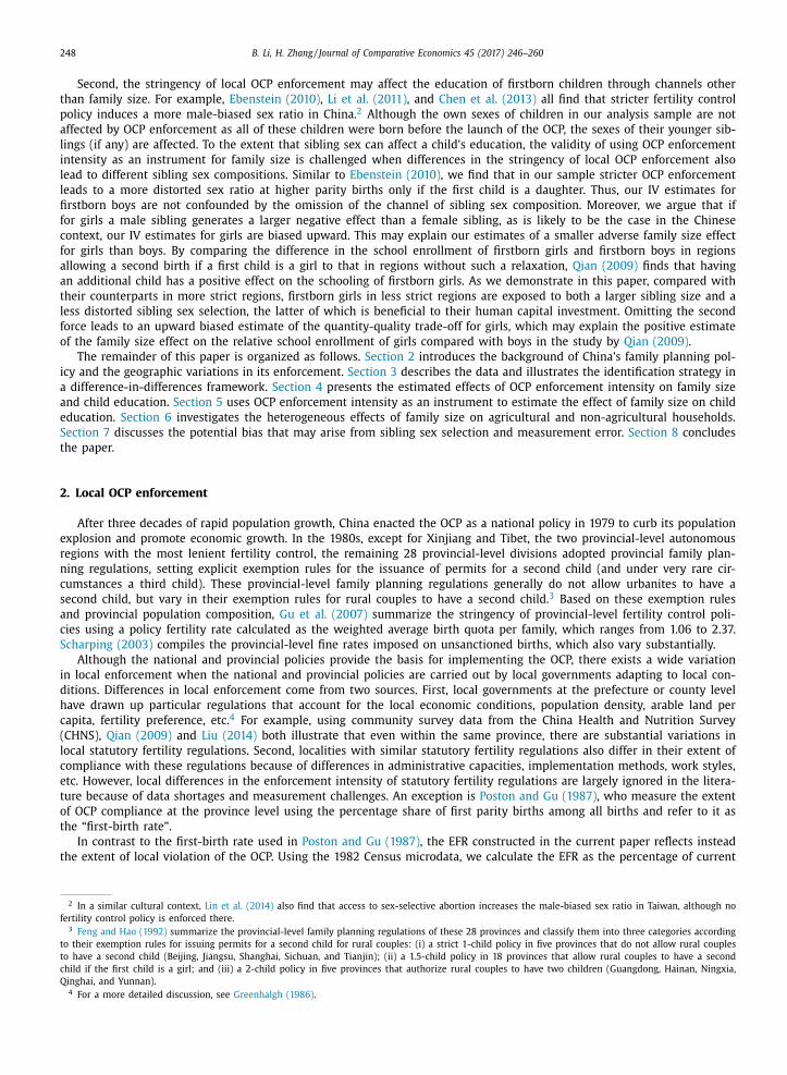
To examine whether the EFR-fertility link indeed differs by age, we estimate the following regression using all Han

females aged 33–57 in the two census years: 12

TotalBirths i jt =

57 ∑

l=33

(EF R j × T i × d il ) θl + W 1 i ζ +

57 ∑

l=33

( C j × T i × d il ) κl + φ j + λt + v i jt , (2)

where TotalBirths i jt is the total number of births of female i in prefecture j from census year t; d il is a dummy that equals

1 if she is aged l ; W 1i contains dummy indicators for education level and employment sector; and C j , T i , φj , and λt are the

same as defined for Eq. (1) . The coefficient θ l reflects the age-specific relationship between a prefecture’s change in fertility

of women aged l from 1982 to 1990 and its EFR. Fig. 1 plots the point estimates and 95% confidence intervals of θ l , which

12 This age range includes 99% of the mothers in our sample.


shows a clear pattern of heterogeneous responses by age. The coefficients are positive and significant for all women aged 45

or below in 1990, who were at their primary childbearing age (i.e., aged 35 or below) when the OCP was officially enacted

in 1980. Moreover, the coefficients almost decrease monotonically with a woman’s age in 1990, which is adversely related

to the length of her childbearing period exposed to the OCP. Third, OCP enforcement intensity is found to have a much

smaller and often insignificant effect on the fertility of women aged 46 or above in 1990, who had passed their primary

childbearing age when the OCP was enacted. We take the results in Fig. 1 as evidence in favor of a causal interpretation of

the first-stage relationship between the EFR and family size.

4.2. Effect of policy enforcement intensity on education

In this subsection, we evaluate the effect of policy enforcement intensity on a firstborn child’s educational outcome by

estimating the following equation:

y i jt = (EF R j × T i ) α2 + X i γ2 + ( C j × T i ) δ2 + φ j + λt + μi jt , (3)

where y ijt denotes the educational outcome of firstborn child i from prefecture j in census year t. T i , X i , C j , φj , and λt are

the same as defined for Eq. (1) . Our measures of educational outcomes include both a discrete indicator for the highest

education level attained and a dummy indicator for junior secondary school attendance. We include an indicator for junior

secondary school attendance separately because it is likely to be the most discernible margin for a child’s education invest-

ment decision made by parents in our sample, as most areas in the country had not achieved nine-year universal education

during our analysis period.

The gender-specific estimation results are reported in Columns 2- and 3, and 5 and 6 of Table 3 . The EFR has a significant

negative effect on a firstborn child’s education level for both genders. The estimates of the coefficient α2 imply that a one-

percentage-point increase in the EFR decreases the education level by 0.005 for firstborn boys and 0.004 for firstborn girls.

The former estimate is significant at the 5% level; the latter estimate, although not significant at conventional levels, has

a p -value of 0.106. More precise estimates are obtained when junior secondary school attendance is used as the outcome

measure: a one-percentage-point higher EFR is associated with a 0.54-percentage-point lower probability of attending junior

secondary school for boys and a 0.63-percentage-point lower probability for girls, both of which are significant at the 1%

level.

Our estimates of the coefficient α2 would be confounded if OCP enforcement intensity were correlated with other omit-

ted time-varying, region-specific determinants of children’s education, such as changes in local school provision and enforce-

ment of nine-year universal education prescribed by the Compulsory Schooling Law. To address this concern, we further

investigate the relationship between the EFR and children’s education level by mother’s age. As the fertility response to the

EFR is larger for younger women than older women, if the negative relationship between a prefecture’s EFR and children’s

education level is driven by the quantity-quality trade-off, then we expect a more lenient OCP enforcement (i.e., higher EFR)

to exert a more severe adverse effect on children of younger mothers than on those of older mothers. Otherwise, if the

negative relationship between a prefecture’s EFR and children’s education level is instead driven by the correlation between

the EFR and other time-varying, region-specific determinants of education, then we expect the spurious negative correlation

between the EFR and education level to hold for all children, regardless of their mother’s age (i.e., the extent to which their

family size might have been affected by the OCP).

We use all 14- to 17-year-old Han children (regardless of birth order) with mothers aged between 33 and 57 in the two

census years to estimate the following regression:

EduLevel i jt =

57 ∑

l=33

(EF R j × T i × d il ) δl + W 2 i ψ +

57 ∑

l=33

( C j × T i × d il ) τl + φ j + λt + υi jt , (4)

where EduLevel i jt is the education level of child i from prefecture j in census year t; d il is a dummy that equals 1 if the

mother is aged l ; W 2i contains a set of individual controls, including dummy indicators for child’s gender and age, mother’s

age, mother’s age squared, and mother’s education level and employment sector; and C j , T i , φj , and λt are the same as

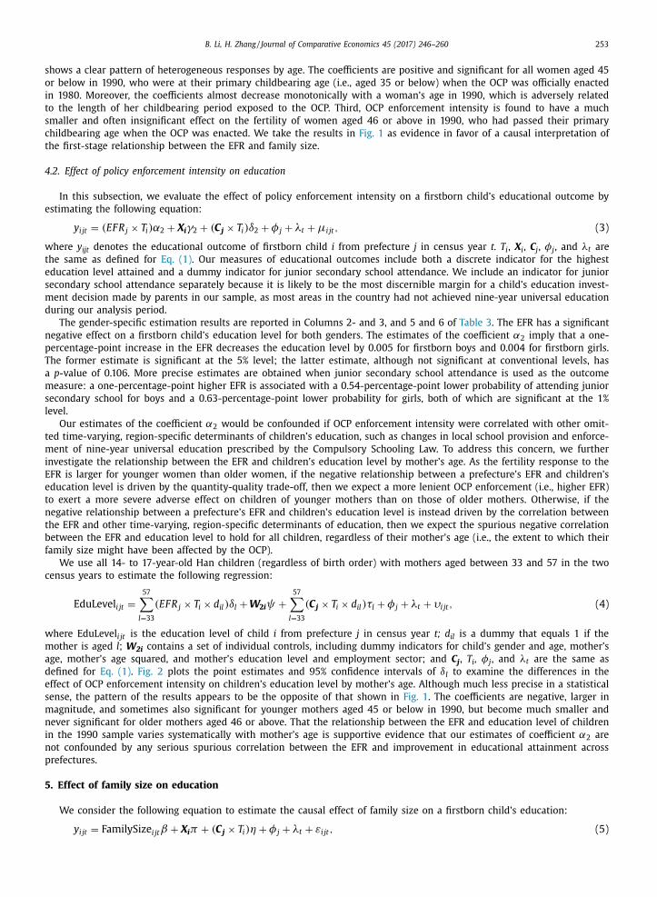
defined for Eq. (1) . Fig. 2 plots the point estimates and 95% confidence intervals of δl to examine the differences in the

effect of OCP enforcement intensity on children’s education level by mother’s age. Although much less precise in a statistical

sense, the pattern of the results appears to be the opposite of that shown in Fig. 1 . The coefficients are negative, larger in

magnitude, and sometimes also significant for younger mothers aged 45 or below in 1990, but become much smaller and

never significant for older mothers aged 46 or above. That the relationship between the EFR and education level of children

in the 1990 sample varies systematically with mother’s age is supportive evidence that our estimates of coefficient α2 are

not confounded by any serious spurious correlation between the EFR and improvement in educational attainment across

prefectures.

5. Effect of family size on education

We consider the following equation to estimate the causal effect of family size on a firstborn child’s education:

y i jt = FamilySize i jt β + X i π + ( C j × T i ) η + φ j + λt + ε i jt , (5)


−2

−1.

5−

1−

.50

.51

33 34 35 36 37 38 39 40 41 42 43 44 45 46 47 48 49 50 51 52 53 54 55 56 57Mother’s Age

Fig. 2. EFR and intercensus change in children’s education level by mother’s age.

Notes: The figure displays the estimated coefficients and 95% confidence intervals of δl of Eq. (4) using 14- to 17-year-old Han children with mothers aged

between 33 and 57 in the 1982 and 1990 Censuses.

Table 4

Effect of family size on firstborn children’s education.

Boys Girls

Education Junior secondary Education Junior secondary

level school attendance level school attendance

(1) (2) (3) (4) (5) (6) (7) (8)

OLS 2SLS OLS 2SLS OLS 2SLS OLS 2SLS

Family size −0.033 ∗∗∗ −0.119 ∗∗ −0.020 ∗∗∗ −0.133 ∗∗∗ −0.078 ∗∗∗ −0.070 ∗ −0.047 ∗∗∗ −0.111 ∗∗∗

(0.003) (0.048) (0.002) (0.039) (0.003) (0.042) (0.002) (0.027)

Control variables:

Individual controls Y Y Y Y Y Y Y Y

Prefecture initial Y Y Y Y Y Y Y Y

controls ×Year1990

Kleibergen and Paap rk statistic 121.26 121.26 210.64 210.64

Stock- Y ogo critical 16.38 16.38 16.38 16.38

value 10% maximal IV size

N 120,273 120,273 120,273 120,273 115,637 115,637 115,637 115,637

Notes: 1 All regressions include prefecture fixed effects and census fixed effects. 2 Individual controls include mother’s age at first birth,

mother’s age at first birth squared, mother’s education level, father’s education level, mother’s employment sector, father’s employment

sector, and child age fixed effects. 3 Pref ecture-specific initial control variables include the average total number of births of females aged

45–54; the shares of females aged 25–44 with 1, 2, 3, and 4+ births, respectively; the shares of females aged 25–29, 30–34, 35–39, and 40–

44, respectively; the agricultural sector’s employment share among adults aged 25–49 by gender; and the shares of each education level

category among adults aged 25–49 by gender. 4 Robust standard errors clustered at prefecture × year level are reported in parentheses. 5 ∗∗∗ p < 0.01, ∗∗ p < 0.05, ∗ p < 0.1.

where y ijt and FamilySize i jt denote, respectively, the educational outcome and family size of firstborn child i from prefecture

j in census year t , and X i , C j , T i , φj , and λt are the same as defined for Eq. (1) .

The odd columns of Table 4 report the gender-specific OLS estimates of Eq. (5) using both the highest education level

attained and junior secondary school attendance as the educational outcome measures. Having an additional sibling is as-

sociated with a lower education level and a lower probability of attending junior secondary school for both boys and girls.

However, the results obtained by OLS may be confounded by the endogeneity between FamilySize i jt and error term ε ijt , as

they are both subject to influences of unobserved parental heterogeneity. However, under the identification assumption that

OCP enforcement intensity has no effect on a firstborn child’s education other than through the channel of family size, we

use the exogenous variation in family size induced by the interaction between local OCP enforcement intensity and census

cohort to estimate the causal effect of family size. The results in Columns 1 and 4 of Table 3 also demonstrate that this

instrument has a good explanatory power in the first stage.

The even columns of Table 4 present the two-stage least squares (2SLS) estimates of Eq. (5) using EFR j × T i as the

instrument. Regardless of the outcome variable and subsample used, the IV estimates of β are always negative and signif-

icant, suggesting that a larger family size always decreases a firstborn child’s education. For boys, the 2SLS point estimates


Table 5

Effect of family size on firstborn children’s education, agricultural households vs. non-agricultural households.

Agricultural households Non-agricultural households

Boy Girl Boy Girl

Family size Family size Family size Family size

(1) (2) (3) (4)

Panel A: First stage

EFR ×Year1990 4.626 ∗∗∗ 6.252 ∗∗∗ 2.179 ∗∗∗ 3.808 ∗∗∗

(0.463) (0.436) (0.535) (0.639)


Stock-Yogo critical 16.38 16.38 16.38 16.38


N 83,129 80,143 37,144 35,494

Junior Junior Junior Junior

Education secondary Education secondary Education secondary Education secondary

level school level school level school level school

attendance attendance attendance attendance

(5) (6) (7) (8) (9) (10) (11) (12)

Panel B: Second stage

Family size −0.091 ∗ −0.112 ∗∗∗ −0.066 ∗ −0.097 ∗∗∗ −0.364 ∗∗ −0.211 ∗∗ −0.101 −0.155 ∗∗∗

(0.047) (0.041) (0.038) (0.027) (0.165) (0.100) (0.096) (0.056)

Control variables:



controls ×Year1990

N 83,129 83,129 80,143 80,143 37,144 37,144 35,494 35,494

Notes: 1 All regressions include prefecture fixed effects and census fixed effects. 2 Individual controls include mother’s age at first birth, mother’s

age at first birth squared, mother’s education level, father’s education level, mother’s employment sector, father’s employment sector, and child age

fixed effects. 3 Pref ecture-specific initial control variables include the average total number of births of females aged 45–54; the shares of females

aged 25–44 with 1, 2, 3, and 4+ births, respectively; the shares of females aged 25–29, 30–34, 35–39, and 40–44, respectively; the agricultural

sector’s employment share among adults aged 25–49 by gender; and the shares of each education level category among adults aged 25–49 by gender. 4 Robust standard errors clustered at prefecture × year level are reported in parentheses. 5 ∗∗∗ p < 0.01, ∗∗ p < 0.05, ∗ p < 0.1.

imply that having an additional sibling decreases their education level by 0.12 and probability of attending junior secondary

school by 13.3 percentage points. The corresponding estimates for girls are somewhat smaller: 0.07 for education level and

11.1 percentage points for junior middle school attendance.

6. Heterogeneous effects between agricultural and non-agricultural households

In Table 5 , we further explore the heterogeneous effects of family size for agricultural and non-agricultural households.

The distinction is based on whether the male head of the household is employed in the agricultural sector. Panel A presents

the first-stage results for different samples. Consistent with our baseline results in Table 3 , a positive relationship between

the EFR and family size is found for all of the samples. However, regardless of gender, the effect is estimated to be much

larger for the agricultural households than the non-agricultural households. For example, a one-percentage-point increase in

the EFR is associated with a 0.063 higher family size among agriculture households with a firstborn girl but only a 0.038

higher family size among non-agricultural households with a firstborn girl.

Panel B presents the IV regression results across the samples. Consistent with the results in Table 4 , we find that family

size has negative effects across all of the samples. For girls, the estimated effect of family size is similar between agricultural

households and non-agricultural households. For boys, although the effect of family size is always quantitatively larger for

non-agricultural households than agricultural households, their equality can never be rejected with statistical significance.

However, the estimated quantity-quality trade-off for boys in non-agricultural households must be interpreted with caution:

the Kleibergen-Paap rk Wald F statistic falls below the Stock-Yogo critical value for 10% maximal IV size (both of which are

reported in the bottom of Panel A of Table 5 ), suggesting that the estimate may be subject to a weak instrument problem.

7. Robustness

7.1. Sex selection

As we restrict our sample to children born before the launch of the OCP, i.e., the 1965–1968 birth cohorts in the 1982

Census and the 1973–1976 birth cohorts in the 1990 Census, their own sexes were not affected by the OCP. Moreover,

ultrasound machines were not adopted in scale in China until the early 1980s ( Zeng et al., 1993; Chen et al., 2013 ), which

also renders it impossible to conduct prenatal sex selection based on sex-determination technology for these birth cohorts.


Table 6

Sex selection.

Boys Girls

2nd child 3rd child % of male 2nd child 3rd child % of male

is a boy is a boy siblings is a boy is a boy siblings

(1) (2) (3) (4) (5) (6)

EFR ×Year1990 0.052 0.166 0.146 −0.137 −0.288 ∗∗∗ −0.178 ∗∗

(0.117) (0.159) (0.095) (0.107) (0.111) (0.081)

Control variables:



controls ×Year1990

N 113,056 68,311 113,056 110,988 77,553 110,988

Notes: 1 All regressions include prefecture fixed effects and census fixed effects. 2 Individual controls

include mother’s age at first birth, mother’s age at first birth squared, mother’s education level, father’s

education level, mother’s employment sector, father’s employment sector, and child age fixed effects. 3 Prefecture-specific initial control variables include the average total number of births of females aged

45–54; the shares of females aged 25–44 with 1, 2, 3, and 4+ births, respectively; the shares of females

aged 25–29, 30–34, 35–39, and 40–44, respectively; the agricultural sector’s employment share among

adults aged 25–49 by gender; and the shares of each education level category among adults aged 25–

49 by gender. 4 Robust standard errors clustered at prefecture × year level are reported in parentheses. 5 ∗∗∗ p < 0.01, ∗∗ p < 0.05, ∗ p < 0.1.

As a result, for both census samples, the sex ratio was around 104 boys per 100 girls among firstborn children aged 14–

17, showing no evidence of social and behavioral interference. 13 However, the sexes of their younger siblings (if any) were

subject to sex selection due to OCP enforcement and the accessibility of sex-determination technology. For example, the sex

ratio of their younger siblings was 107.9 for the 1982 sample and 111.3 for the 1990 sample, suggesting the existence and

rise of prenatal sex selection among their siblings. Several prior studies find that the extent of sex selection also depends on

the strictness of local fertility control enforcement. Exploiting variations in the fines levied for unauthorized births across

provinces and years, Ebenstein (2010) shows that higher fine regimes are associated with not only lower fertility levels but

also higher sex ratios. Using birth rate as a proxy for county-level intensity of fertility control, Chen et al. (2013) find that

higher-order births are more likely to be male in counties governed by more stringent fertility control enforcement. 14

The literature documents several possible channels through which sibling sex can affect parental human capital invest-

ment in a child (see, e.g., Behrman et al., 1982; 1986; Butcher and Case, 1994 ). The validity of our IV strategy to identify

the causal effect of family size on child education hinges on the assumption that family size is the only channel through

which prefectural differences in OCP enforcement intensity affect child education. However, if differences in the strictness

of local OCP enforcement also lead to differences in the sibling sex composition, which has its own effect on a child’s ed-

ucation, then the 2SLS estimates reported in Table 4 are biased due to the omission of the sibling sex channel. Ebenstein

(2010) documents that sex ratio distortions exist at higher parity births only if the first child is a daughter. If that is indeed

the case, we will only be concerned about biases in the estimates for firstborn girls. To examine the empirical relationship

between the sexes of younger siblings (if any) and local OCP enforcement intensity based on the firstborn child’s gender, we

estimate the following regression:

SibSex i jt = (EF R j × T i ) α3 + X i γ3 + ( C j × T i ) δ3 + φ j + λt + u i jt . (6)

The specification of Eq. (6) is the same as that of Eq. (1) except that the dependent variable is a measure of sibling sex, for

which we use a dummy indicator for a male second/third birth or the fraction of male siblings.

Table 6 shows the results estimated separately for firstborn boys (Columns 1–3) and firstborn girls (Columns 4–6) in our

sample. Like Ebenstein (2010) , we find no relationship between sibling sexes and the stringency of local OCP enforcement

when the first child is a son, suggesting that our IV estimates of the quantity-quality trade-off for boys are not confounded

by the omission of sibling sex composition. While we do find evidence that stricter fertility control leads to a more distorted

sex ratio at higher parity births when the first child is a daughter, the magnitude of the effect of the EFR on sibling sex

composition is much smaller than that on family size. A one-percentage-point reduction in the EFR is associated with a

0.14(0.29)-percentage-point higher probability of having a male second (third) birth or a 0.18-percentage-point increase in

the percentage of male siblings. Given the latter estimate, the difference in the mean EFR between strict regions (i.e., 5.8%)

and non-strict regions (i.e., 9.1%) increases the fraction of male siblings by only 0.69 percentage point. Although sex selection

is widespread in the country, the bias from such a small extent of differential sex selection caused by local OPC enforcement

13 According to statistics from developed countries with reliable data covering over the past 200 years, Johansson and Nygren (1991) indicate that the

expected sex ratio among live births under normal circumstances is between 105 and 106 boys per 100 girls. 14 In addition, Chen et al. (2013) also find that local access to ultrasound technology has a larger positive effect on male probability for higher-order births

in areas with stricter enforcement of OCP.


intensity in the estimated family size effect on a firstborn child’s education is likely to be modest at most. Moreover, in the

Chinese context, it is plausible to assume that, for firstborn girls, having a male sibling generates a more negative effect

on human capital investment than having a female sibling. As more relaxed fertility control (i.e., a higher EFR) leads to a

larger family size but lower chances of having a male sibling, our IV estimates of the family size effect for firstborn girls,

which omit the effect through the second channel, are biased upward. That is, given the negative sign of our IV estimator,

its absolute value puts a lower bound on the magnitude of the adverse effect of family size on firstborn girls’ education.

The presence of upward bias in the IV estimator for the firstborn girl sample may explain why we always obtain a smaller

estimate of the adverse effect of family size for girls than for boys.

7.2. Measurement

As shown in Appendix A , the EFR is measured as the percentage of current mothers of primary childbearing age who

gave a higher order birth in 1981. One may be concerned about a mechanical correlation between the EFR and family size

in our analysis as mothers in our sample (some of whom actually gave birth in 1981) are also used in calculating the EFR.

To alleviate this concern, we construct an alternative EFR measure excluding mothers in our sample. That is, this alternative

EFR is calculated as the percentage of current mothers of primary childbearing age with firstborn children not in the age

groups 6–9 15 and 14–17 in 1982 who gave a higher order birth in 1981. 16 We replicate the regressions in Tables 3 and

4 using this alternative EFR and report the results in Tables A1 and A2 . All estimates in Tables A1 and A2 are qualitatively

the same as those in Tables 3 and 4 , showing that our findings are robust to the use of this alternative EFR.

Another measurement concern for the EFR is that it may be subject to measurement error due to birth underreporting, a

phenomenon documented to widely exist in China (e.g., Merli and Raftery, 20 0 0; Scharping, 20 03; Retherford et al., 2005 ).

Moreover, measurement error in the EFR at the prefecture level and that in the reported family size at the household level

are almost certainly positively correlated with each other. In Appendix B , we show that correlated measurement errors in

the endogenous variable and instrument yield a multiplicative bias to the IV estimate but do not change its sign. Therefore,

our finding of the existence of a quantity-quality trade-off is robust to the potential presence of such a multiplicative bias.

Moreover, the bias is likely to be attenuative in nature under some plausible assumption about households’ underreporting

behavior, making the IV estimate yield an upper bound for the extent of the quantity-quality trade-off when it exists.

8. Conclusion

In this paper, we investigate the effect of family size on children’s education in China using the 1982 and 1990 Census

microdata. Exploiting the fact that family size in the 1990 sample was subject to much greater influence of the OCP than

the 1982 sample, we use a prefecture’s OCP enforcement intensity, measured by its EFR in 1981, as an exogenous source of

variation for its family size in the 1990 sample. Complementary to the earlier literature, we find evidence of the existence

of the quantity-quality trade-off in the Chinese context. When education level is used as the outcome measure, our results

indicate that an additional sibling decreases the education level by 0.12 for boys and 0.07 for girls. These estimates are

most directly comparable to those of Li et al. (2008) , who also use the 1990 Census to examine the effect of family size on

children’s education level, but instead exploit exogenous variations in family size from the natural occurrences of twins. They

find that additional sibling due to a twin birth lowers a non-twin child’s education level by 0.04. The disparity between our

estimates and theirs is most likely due to differences in sample selection. Their child sample consists of all children aged

7–17, and we restrict our sample to older children aged 14–17 only. As the schooling decisions of primary-school-aged

children (i.e., 7–13 years of age) are likely to be much less sensitive to family size than those of secondary-school-aged

children (i.e., 14–17 years of age), the quantity-quality trade-off is expected to be more discernible in our sample.

While our results support the claim that China’s OCP enhances the human capital investment in children through the

quantity-quality trade-off channel, to estimate the effect of the OCP on human capital accumulation, one also needs to gauge

the effect of the OCP on fertility. As Table 1 shows, the average family size in our analysis sample decreased from 3.59 in

1982 to 2.60 in 1990. Although we probably cannot attribute this decline entirely to the OCP, it nevertheless provides an

upper bound for the policy effect. As obtaining a higher education level beyond primary school on average requires three

extra years of schooling, our estimated effect of family size on education level indicates that an additional sibling decreases

years of schooling by 0.36 years for boys and 0.21 years for girls. Using the observed fertility decline between the two

census years (i.e., one less child) as the upper bound of the OCP effect on fertility, our estimates imply that the OCP at

most increased years of schooling by 0.36 years for boys and 0.21 years for girls. Zhang et al. (2005) estimate the returns

to an additional year of schooling in urban China at 10.2% in 2001, which is among the highest estimates in the literature.

Combining the estimate of the rate of returns to schooling in Zhang et al. (2005) and our upper-bound estimate of the

policy effect on schooling suggests that the OCP at most increased men’s income by 3.7% and women’s income by 2%. Using

fertility survey data, McElroy and Yang (20 0 0) show that after controlling for county-level monetary penalties on above-

quota births, women married during the OCP regime (1980–1991) averaged only half a child less than those married before

15 Firstborn children aged 6–9 in 1982 turned 14–17 in 1990 and belong to the 1990 sample. 16 By excluding mothers in our sample from both the numerator and denominator in calculating it, this alternative EFR is no longer mechanically corre-

lated with the family size in our sample.


1971. If we use their estimate that the OCP decreased family size by only half a child, then the corresponding policy effect

on both education and income will also be halved. Overall, despite evidence for the existence of the quantity-quality trade-

off in China, our quantitative estimates suggest that China’s OCP made only a modest contribution to the human capital

development and income growth of its labor force, which is in line with the conclusions reached by Rosenzweig and Zhang

(2009) and Liu (2014) .

Appendix A. EFR calculation

As discussed in Section 2 , the EFR in a locality is defined as the percentage of its current Han mothers (i.e., women

with at least one surviving child) aged 25–44 who gave a higher order birth in 1981. Thus, to calculate the EFR, we need

to identify both the number of second or higher parity births by Han women aged 25–44 in 1981 (i.e., the numerator)

and the number of Han women aged 25–44 with at least one surviving child born before 1981 (i.e., the denominator). This

Table A1

Effect of policy enforcement intensity on family size and firstborn children’s education (alternative EFR).

Boys Girls

Junior Junior

Family Education secondary Family Education secondary

size level school size level school

attendance attendance

(1) (2) (3) (4) (5) (6)

Alternative EFR ×Year1990 3.227 ∗∗∗ −0.494 ∗∗∗ −0.555 ∗∗∗ 4.991 ∗∗∗ −0.437 ∗ −0.704 ∗∗∗

(0.367) (0.183) (0.146) (0.409) (0.238) (0.149)

Control variables:



controls ×Year1990

N 120,273 120,273 120,273 115,637 115,637 115,637

Notes: 1 All regressions include prefecture fixed effects and census fixed effects. 2 Individual controls include

mother’s age at first birth, mother’s age at first birth squared, mother’s education level, father’s education

level, mother’s employment sector, father’s employment sector, and child age fixed effects. 3 Prefecture-specific

initial control variables include the average total number of births of females aged 45–54; the shares of females

aged 25–44 with 1, 2, 3, and 4+ births, respectively; the shares of females aged 25–29, 30–34, 35–39, and

40–44, respectively; the agricultural sector’s employment share among adults aged 25–49 by gender; and the

shares of each education level category among adults aged 25–49 by gender. 4 Robust standard errors clustered

at prefecture × year level are reported in parentheses. 5 ∗∗∗ p < 0.01, ∗∗ p < 0.05, ∗ p < 0.1.

Table A2

Effect of family size on firstborn children’s education (alternative EFR).

Boys Girls

Education Junior secondary Education Junior secondary

level school attendance level school attendance

(1) (2) (3) (4) (5) (6) (7) (8)

OLS 2SLS OLS 2SLS OLS 2SLS OLS 2SLS

Family size −0.033 ∗∗∗ −0.153 ∗∗ −0.020 ∗∗∗ −0.172 ∗∗∗ −0.078 ∗∗∗ −0.088 ∗ −0.047 ∗∗∗ −0.141 ∗∗∗

(0.003) (0.060) (0.002) (0.051) (0.003) (0.046) (0.002) (0.029)

Control variables:



controls ×Year1990


Stock-Yogo critical 16.38 16.38 16.38 16.38


N 120,273 120,273 120,273 120,273 115,637 115,637 115,637 115,637

Notes: 1 All regressions include prefecture fixed effects and census fixed effects. 2 Individual controls include mother’s age at first birth,

mother’s age at first birth squared, mother’s education level, father’s education level, mother’s employment sector, father’s employment

sector, and child age fixed effects. 3 Pref ecture-specific initial control variables include the average total number of births of females aged

45–54; the shares of females aged 25–44 with 1, 2, 3, and 4+ births, respectively; the shares of females aged 25–29, 30–34, 35–39, and

40–44, respectively; the agricultural sector’s employment share among adults aged 25–49 by gender; and the shares of each education level

category among adults aged 25–49 by gender. 4 Robust standard errors clustered at prefecture × year level are reported in parentheses. 5 ∗∗∗

p < 0.01, ∗∗ p < 0.05, ∗ p < 0.1.


appendix provides the formula and discusses the details for calculating the EFR at the prefecture level using the 1982 Census

microdata.

For woman i from prefecture j , let Birth i j denote a dummy indicator for whether she gave a birth in 1981 and NSC i j

denote her number of surviving children by the end of 1981. Then, the number of excess births (i.e., second or higher

parity births) in prefecture j can be calculated as ∑

i

(Birth i j · 1 ( NSC i j ≥ 2)

)for all Han women aged 25–44. To identify the

number of women at potential risk of violating the OCP at the beginning of 1981, we need to exclude new mothers who

gave their first birth in 1981 (i.e., Birth i j = 1 and NSC i j = 1 ) from all existing mothers at the end of 1981 (i.e., NSC i j ≥ 1 ),

i.e., ∑

i

1 ( NSC i j ≥ 1) − ∑

i

( Birth i j · 1 ( NSC i j = 1)) . Therefore, the EFR of prefecture j can be calculated by applying the following

formula to all women aged 25–44:

EF R j =

∑

i

(Birth i j · 1 ( NSC i j ≥ 2)

)∑

i

1 ( NSC i j ≥ 1) −∑

i

( Birth i j · 1 ( NSC i j = 1)) . (A1)

Although the 1982 Census microdata directly contains information on a woman’s fertility status in 1981 (i.e., Birth i j ), it

only records a woman’s number of surviving children at the time of the census (i.e., July 1, 1982). So in practice, we have to

make an approximation to use NSC i j at mid-1982 to proxy for NSC i j at end-1981. As the results of this approximation, the

numerator used is the number of women who gave a birth in 1981 and had two or more children at mid-1982 (ideally at

end-1981), and the denominator used is the number of mothers at mid-1982 (ideally at end-1981) minus those who gave a

birth in 1981 and had only one child at mid-1982 (ideally at end-1981).

Appendix B. Measurement error due to birth underreporting

Birth underreporting is documented to widely exist in China, which may lead to measurement errors in both the en-

dogenous variable family size and its instrument EFR. Although measurement errors in the endogenous variable/instrument

alone do not usually lead to inconsistent IV estimates, they do in our context because measurement errors in reported

family size at the household level and measurement errors in the reported EFR at the prefecture level are almost certainly

positively correlated with each other. In this appendix, we show that correlated measurement errors in family size and EFR

yield a multiplicative bias in the IV estimate, but nonetheless leave its sign unchanged compared with the quantity-quality

trade-off parameter of interest.

Let reported family size (denoted by x ), actual family size (denoted by x ∗), and extent of underreporting at the household

level ( e x ) have the following relationship:

x = x ∗ − e x ,

where e x ≥ 0. Let us assume that the underlying linear relationship between outcome y and actual family size x ∗ is given

by

y = α + βx ∗ + μ,

where u is the individual-level error term. Then, the relationship between outcome y , reported family size x , and underre-

porting e x is given by

y = α + βx + βe x + μ︸︷︷︸ ε

. (A2)

Analogously define z reported EFR, z ∗ actual EFR, and e z underreporting of EFR at the prefecture level, such that

z = z ∗ − e z ,

where e z ≥ 0. Here, we assume that both z ∗ and e z are orthogonal to μ (i.e., σz ∗μ = 0 and σe z μ = 0 ), 17 such that σzu = 0 ,

although we still allow z to be correlated with the error term ε in Eq. (A2) through βe x .

Then, the IV estimator can be expressed as

β IV =

Cov (z, y )

Cov (z, x ) =

Cov (z, α + βx ∗ + μ)

Cov (z, x ) =

σzx ∗

σzx β. (A3)

Our estimate of a strong positive first-stage relationship between reported family size ( x ) and reported EFR ( z ) indicates σ zx

> 0. It is also plausible to assume that actual family size ( x ∗) is positively correlated with reported EFR ( z ), i.e., σzx ∗ > 0 .

(Note that a negative correlation between x ∗ and z would imply that actual family sizes are larger in prefectures with lower

reported EFRs but smaller in prefectures with higher reported EFRs, which seems highly implausible.) When σzx ∗ and σ zx

are both positive, Eq. (A3) indicates that correlated measurement errors in x and z yield a multiplicative bias only, which

makes the sign of β IV the same as that of β . Thus, our finding of the existence of a quantity-quality trade-off (i.e., β < 0)

is unaffected by the presence of this multiplicative bias, although it may affect the magnitude of our IV estimate.

17 Specific to our context, this requires that both the actual EFR and its measurement error be uncorrelated with the time-varying, region-specific deter-

minants of children’s educational outcomes.


To consider the size effect of the multiplicative bias on the IV estimate, we can rewrite Eq. (A3) as follows:

β IV =

σzx ∗

σzx β = (1 +

σze x

σzx ) β = (1 +

σz ∗e x − σe z e x

σzx ) β. (A4)

It is natural to assume that the covariance between e z and e x is positive, i.e., σe z e x > 0 . Therefore, as long as the household-

level birth underreporting ( e x ) has a larger covariance with the prefecture-level EFR underreporting ( e z ) than with the

prefecture-level actual EFR ( z ∗), i.e., σe z e x > σz ∗e x (which includes σz ∗e x = 0 as a special case), the bias in the IV estimator

in Eq. (A4) will be attenuative in nature, making β IV yield an upper bound for β when the quantity-quality trade-off exists

(i.e., β < 0).

References

Angrist, J. , Lavy, V. , Schlosser, A. , 2010. Multiple experiments for the causal link between the quantity and quality of children. J. Labor Econ. 28 (4), 773–823 .

Becker, G.S. , 1960. An economic analysis of fertility. In: Becker, G.S. (Ed.), Demographic and Economic Change in Developed Countries. Princeton UniversityPress, Princeton, NJ .

Becker, G.S. , Lewis, H.G. , 1973. On the interaction between the quantity and quality of children. J. Political Econ. 81 (2), 279–288 . Becker, G.S. , Tomes, N. , 1976. Child endowments and the quantity and quality of children. J. Political Econ. 84 (4), 143–162 .

Behrman, J.R. , Pollak, R.A. , Taubman, P. , 1982. Parental preferences and provision for progeny. J. Political Econ. 90 (1), 52–73 . Behrman, J.R. , Pollak, R.A. , Taubman, P. , 1986. Do parents favor boys? Int. Econ. Rev. 27 (1), 33–54 .

Black, S.E. , Devereux, P.J. , Salvanes, K.G. , 2005. The more the merrier? the effect of family size and birth order on children’s education. Q. J. Econ. 120 (2),

669–700 . Blake, J. , 1989. Family Size and Achievement. University of California Press, Berkeley and Los Angeles, CA .

Butcher, K.F. , Case, A. , 1994. The effect of sibling sex composition on women’s education and earnings. Q. J. Econ. 109 (3), 531–563 . Cáeres-Delpiano, J. , 2006. The impacts of family size on investment in child quality. J. Hum. Resour. 41 (4), 738–754 .

Chen, Y. , Li, H. , Meng, L. , 2013. Prenatal sex selection and missing girls in China. J. Hum. Resour. 48 (1), 36–70 . Duflo, E. , 2001. Schooling and labor market consequences of school construction in indonesia: evidence from an unusual policy experiment. Am. Econ. Rev.

91 (4), 795–813 .

Ebenstein, A. , 2010. The “missing girls” of China and the unintended consequences of the one child policy. J. Hum. Resour. 45 (1), 87–115 . Feng, G. , Hao, L. , 1992. Review of the twenty-eight local family planning regulations. Popul. Studies 4 (3), 381–394 . (in Chinese).

Fitzsimons, E. , Malde, B. , 2014. Empirically probing the quantity-quality model. J. Popul. Econ. 27 (1), 33–68 . Greenhalgh, S. , 1986. Shifts in China’s population policy, 1984–1986: views from the central, provincial, and local levels. Popul. Dev. Rev. 64 (2), 169–187 .

Gu, B. , Wang, F. , Guo, Z. , Zhang, E. , 2007. China’s local and national fertility policies at the end of the twentieth century. Popul. Dev. Rev. 33 (1), 129–147 . Hazan, M. , Berdugo, B. , 2002. Child labour, fertility, and economic growth. Econ. J. 112 (482), 810–828 .

Johansson, S. , Nygren, O. , 1991. The missing girls of China: a new demographic account. Popul. Dev. Rev. 16 (1), 63–83 .

King, E.M. , 1987. The effect of family size on family welfare: what do we know?. In: Johnson, D.G, Lee, R.D. (Eds.) Population Growth and EconomicDevelopment: Issues and Evidence. University of Wisconsin Press, Madison, WI, pp. 373–412 .

Lee, J. , 2008. Sibling size and investment in children’s education: an asian instrument. J. Popul. Econ. 21 (4), 855–875 . Li, H. , Yi, J. , Zhang, J. , 2011. Estimating the effect of the one-child policy on sex ratio imbalance in china: Identification based on the difference-in-differences.

Demography 48 (4), 1535–1557 . Li, H. , Zhang, J. , Zhu, Y. , 2008. The quantity-quality trade-off of children in a developing country: identification using chinese twins. Demography 45 (1),

223–243 .

Lin, M.-J. , Liu, J.-T. , Qian, N. , 2014. More missing women, fewer dying girls: the impact of sex-selective abortion on sex at birth and relative female mortalityin taiwan. J. Eur. Econ. Assoc. 12 (4), 899–926 .

Liu, H. , 2014. The quality-quantity trade-off: evidence from the relaxation of China’s one-child policy. J. Popul. Econ. 27 (2), 565–602 . McElroy, M. , Yang, D.T. , 20 0 0. Carrots and sticks: Fertility effects and China’s population policies. Am. Econ. Rev. 90 (2), 389–392 .

Merli, M.G. , Raftery, A.E. , 20 0 0. Are births underreported in rural China? Manipulation of statistical records in response to China’s population policies.Demography 37 (1), 109–126 .

Millimet, D.L. , Wang, L. , 2011. Is the quantity-quality trade-off a trade-off for all, none, or some? Econ. Dev. Cult. Change 60 (1), 155–159 .

Moav, O. , 2005. Cheap children and the persistence of poverty. Econ. J. 115 (500), 88–110 . Poston, D.L. , Gu, B. , 1987. Socioeconomic development, family planning, and fertility in China. Demography 24 (4), 531–551 .

Qian, N., 2009. Quantity-Quality and The One Child Policy: The Only-Child Disadvantage in School Enrollment in Rural China. National Bureau of EconomicResearch (NBER) Working Paper 14973.

Retherford, R.D. , Choe, M.K. , Chen, J. , Li, X. , Hongyan, C. , 2005. How far has fertility in China really declined? Popul. Dev. Rev. 31 (1), 57–84 . Rosenzweig, M.R. , Wolpin, K.I. , 1980. Testing the quantity-quality fertility model: The use of twins as a natural experiment. Econometrica 48 (1), 227–240 .

Rosenzweig, M.R. , Zhang, J. , 2009. Do population control policies induce more human capital investment? Twins, Birth Weight and China’s ”One-Child”

Policy. Rev. Econ. Stud. 76 (3), 1149–1174 . Scharping, T. , 2003. Birth Control in China, 1949–2000: Population Policy and Demographic Development. Routledge Curzon, New York, NY .

Stafford, F.P. , 1987. Women’s work, sibling competition, and children’s school performance. Am. Econ. Rev. 77 (5), 972–980 . Zeng, Y. , Tu, P. , Gu, B. , Xu, Y. , Li, B. , Li, Y. , 1993. Causes and implications of the recent increase in the reported sex ratio at birth in China. Popul. Dev. Rev.

19 (2), 283–302 . Zhang, J. , Zhao, Y. , Park, A. , Song, X. , 2005. Economic returns to schooling in urban China, 1988 to 2001. J. Comp. Econ. 33 (4), 730–752 .

http://refhub.elsevier.com/S0147-5967(16)30058-0/sbref0001























































































































journal of comparative economics - hongliang zhang of comparative economics 45 (2017) 246–260 ......

Documents