Learning brain regions via large-scale onlinestructured sparse dictionary-learning

Elvis Dohmatob, Arthur Mensch, Gael Varoquaux, Bertrand Thirionfirstname.lastname@inria.fr

Parietal Team, INRIA / CEA, Neurospin, Université Paris-Saclay, France

Abstract

We propose a multivariate online dictionary-learning method for obtaining de-compositions of brain images with structured and sparse components (aka atoms).Sparsity is to be understood in the usual sense: the dictionary atoms are constrainedto contain mostly zeros. This is imposed via an `1-norm constraint. By "struc-tured", we mean that the atoms are piece-wise smooth and compact, thus making upblobs, as opposed to scattered patterns of activation. We propose to use a Sobolev(Laplacian) penalty to impose this type of structure. Combining the two penalties,we obtain decompositions that properly delineate brain structures from functionalimages. This non-trivially extends the online dictionary-learning work of Mairal etal. (2010), at the price of only a factor of 2 or 3 on the overall running time. Justlike the Mairal et al. (2010) reference method, the online nature of our proposedalgorithm allows it to scale to arbitrarily sized datasets. Preliminary xperimentson brain data show that our proposed method extracts structured and denoiseddictionaries that are more intepretable and better capture inter-subject variability insmall medium, and large-scale regimes alike, compared to state-of-the-art models.

1 Introduction

In neuro-imaging, inter-subject variability is often handled as a statistical residual and discarded. Yetthere is evidence that it displays structure and contains important information. Univariate models areineffective both computationally and statistically due to the large number of voxels compared to thenumber of subjects. Likewise, statistical analysis of weak effects on medical images often relies ondefining regions of interests (ROIs). For instance, pharmacology with Positron Emission Tomography(PET) often studies metabolic processes in specific organ sub-parts that are defined from anatomy.Population-level tests of tissue properties, such as diffusion, or simply their density, are performed onROIs adapted to the spatial impact of the pathology of interest. Also, in functional brain imaging,e.g function magnetic resonance imaging (fMRI), ROIs must be adapted to the cognitive processunder study, and are often defined by the very activation elicited by a closely related process [18].ROIs can boost statistical power by reducing multiple comparisons that plague image-based statisticaltesting. If they are defined to match spatially the differences to detect, they can also improve thesignal-to-noise ratio by averaging related signals. However, the crux of the problem is how to definethese ROIs in a principled way. Indeed, standard approaches to region definition imply a segmentationstep. Segmenting structures in individual statistical maps, as in fMRI, typically yields meaningfulunits, but is limited by the noise inherent to these maps. Relying on a different imaging modality hitscross-modality correspondence problems.

Sketch of our contributions. In this manuscript, we propose to use the variability of the statisticalmaps across the population to define regions. This idea is reminiscent of clustering approaches, thathave been employed to define spatial units for quantitative analysis of information as diverse as brainfiber tracking, brain activity, brain structure, or even imaging-genetics. See [21, 14] and referencestherein. The key idea is to group together features –voxels of an image, vertices on a mesh, fiber tracts–

30th Conference on Neural Information Processing Systems (NIPS 2016), Barcelona, Spain.

based on the quantity of interest, to create regions –or fiber bundles– for statistical analysis. However,unlike clustering that models each observation as an instance of a cluster, we use a model closer tothe signal, where each observation is a linear mixture of several signals. The model is closer to modefinding, as in a principal component analysis (PCA), or an independent component analysis (ICA),often used in brain imaging to extract functional units [5]. Yet, an important constraint is that themodes should be sparse and spatially-localized. For this purpose, the problem can be reformulated asa linear decomposition problem like ICA/PCA, with appropriate spatial and sparse penalties [25, 1].We propose a multivariate online dictionary-learning method for obtaining decompositions withstructured and sparse components (aka atoms). Sparsity is to be understood in the usual sense: theatoms contain mostly zeros. This is imposed via an `1 penalty on the atoms. By "structured", we meanthat the atoms are piece-wise smooth and compact, thus making up blobs, as opposed to scatteredpatterns of activation. We impose this type of structure via a Laplacian penalty on the dictionary atoms.Combining the two penalties, we therefore obtain decompositions that are closer to known functionalorganization of the brain. This non-trivially extends the online dictionary-learning work [16], withonly a factor of 2 or 3 on the running time. By means of experiments on a large public dataset, weshow the improvements brought by the spatial regularization with respect to traditional `1-regularizeddictionary learning. We also provide a concise study of the impact of hyper-parameter selection onthis problem and describe the optimality regime, based on relevant criteria (reproducibility, capturedvariability, explanatory power in prediction problems).

2 Smooth Sparse Online Dictionary-Learning (Smooth-SODL)

Consider a stack X ∈ Rn×p of n subject-level brain images X1,X2, . . . ,Xn each of shape n1 ×n2 × n3, seen as p-dimensional row vectors –with p = n1 × n2 × n3, the number of voxels. Thesecould be images of fMRI activity patterns like statistical parametric maps of brain activation, rawpre-registered (into a common coordinate space) fMRI time-series, PET images, etc. We wouldlike to decompose these images as a mixture of k ≤ min(n, p) component maps (aka latent factorsor dictionary atoms)V1, . . . ,Vk ∈ Rp×1 and modulation coefficientsU1, . . . ,Un ∈ Rk×1 calledcodes (one k-dimensional code per sample point), i.e

Xi ≈ VUi, for i = 1, 2, . . . , n (1)

where V := [V1| . . . |Vk] ∈ Rp×k, an unknown dictionary to be estimated. Typically, p ∼ 105 –106 (in full-brain high-resolution fMRI) and n ∼ 102 – 105 (for example, in considering all the 500subjects and all the about functional tasks of the Human Connectome Project dataset [20]). Ourwork handles the extreme case where both n and p are large (massive-data setting). It is reasonablethen to only consider under-complete dictionaries: k ≤ min(n, p). Typically, we use k ∼ 50 or 100components. It should be noted that online optimization is not only crucial in the case where n/p isbig; it is relevant whenever n is large, leading to prohibitive memory issues irrespective of how big orsmall p is.As explained in section 1, we want the component maps (aka dictionary atoms)Vj to be sparse andspatially smooth. A principled way to achieve such a goal is to impose a boundedness constraint on`1-like norms of these maps to achieve sparsity and simultaneously impose smoothness by penalizingtheir Laplacian. Thus, we propose the following penalized dictionary-learning model

minV∈Rp×k

(limn→∞

1

n

n∑i=1

minUi∈Rk

1

2‖Xi −VUi‖22 +

1

2α‖Ui‖22

)+ γ

k∑j=1

ΩLap(Vj).

subject to V1, . . . ,Vk ∈ C(2)

The ingredients in the model can be broken down as follows:

• Each of the terms maxUi∈Rk1

2‖Xi −VUi‖22 measures how well the current dictionary V

explains dataXi from subject i. The Ridge penalty term φ(Ui) ≡ 12α‖Ui‖22 on the codes

amounts to assuming that the energy of the decomposition is spread across the differentsamples. In the context of a specific neuro-imaging problem, if there are good grounds toassume that each sample / subject should be sparsely encoded across only a few atoms ofthe dictionary, then we can use the `1 penalty φ(Ui) := α‖Ui‖1 as in [16]. We note that in

2

contrast to the `1 penalty, the Ridge leads to stable codes. The parameter α > 0 controls theamount of penalization on the codes.

• The constraint set C is a sparsity-inducing compact simple (mainly in the sense that theEuclidean projection onto C should be easy to comput) convex subset of Rp like an `1-ballBp,`1(τ) or a simplex Sp(τ), defined respectively as

Bp,`1(τ) := v ∈ Rp s.t |v1|+ . . .+ |vp| ≤ τ , and Sp(τ) := Bp,`1(τ) ∩ Rp+. (3)

Other choices (e.g ElasticNet ball) are of course possible. The radius parameter τ > 0controls the amount of sparsity: smaller values lead to sparser atoms.• Finally, ΩLap is the 3D Laplacian regularization functional defined by

ΩLap(v) :=1

2

p∑k=1

(∇xv)2k + (∇yv)2

k + (∇zv)2k =

1

2vT∆v ≥ 0, ∀v ∈ Rp, (4)

∇x being the discrete spatial gradient operator along the x-axis (a p-by-p matrix), ∇y alongthe y-axis, etc., and ∆ := ∇T∇ is the p-by-p matrix representing the discrete Laplacianoperator. This penalty is meant to impose blobs. The regularization parameter γ ≥ 0 controlshow much regularization we impose on the atoms, compared to the reconstruction error.

The above formulation, which we dub Smooth Sparse Online Dictionary-Learning (Smooth-SODL)is inspired by, and generalizes the standard online dictionary-learning framework of [16] –henceforthreferred to as Sparse Online Dictionary-Learning (SODL)– with corresponds to the special caseγ = 0.

3 Estimating the model

3.1 Algorithms

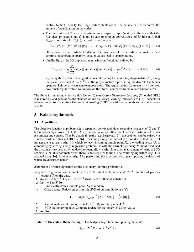
The objective function in problem (2) is separately convex and block-separable w.r.t each ofU andVbut is not jointly convex in (U,V). Also, it is continuously differentiable on the constraint set, whichis compact and convex. Thus by classical results (e.g Bertsekas [6]), the problem can be solved viaBlock-Coordinate Descent (BCD) [16]. Reasoning along the lines of [15], we derive that the BCDiterates are as given in Alg. 1 in which, for each incoming sample point Xt, the loading vector Ut iscomputing by solving a ridge regression problem (5) with the current dictionaryVt held fixed, andthe dictionary atoms are then updated sequentially via Alg. 2. A crucial advantage of using a BCDscheme is that it is parameter free: there is not step size to tune. The resulting algorithm Alg. 1, isadapted from [16]. It relies on Alg. 2 for performing the structured dictionary updates, the details ofwhich are discussed below.

Algorithm 1 Online algorithm for the dictionary-learning problem (2)

Require: Regularization parameters α, γ > 0; initial dictionary V ∈ Rp×k, number of passes /iterations T on the data.

1: A0 ← 0 ∈ Rk×k, B0 ← 0 ∈ Rp×k (historical “sufficient statistics”)2: for t = 1 to T do3: Empirically draw a sample point Xt at random.4: Code update: Ridge-regression (via SVD of current dictionary V)

Ut ← argminu∈Rk1

2‖Xt −Vu‖22 +

1

2α‖u‖22. (5)

5: Rank-1 updates: At ← At−1 + UtUTt , Bt ← Bt−1 + XtU

Tt

6: BCD dictionary update: Compute update for dictionary V using Alg. 2.7: end for

Update of the codes: Ridge-coding. The Ridge sub-problem for updating the codes

Ut = (VTV + αI)−1VTXt (6)

3

is computed via an SVD of the current dictionary V. For α ≈ 0, Ut reduces to the orthogonalprojection of Xt onto the image of the current dictionary V. As in [16], we speed up the overallalgorithm by sampling mini-batches of η samples Xt, . . . ,Xη and compute the corresponding codesU1, U2, ..., Uη at once. We typically use we use mini-batches of size η = 20.

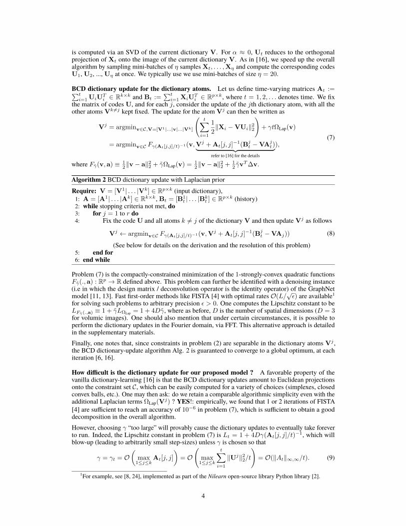
BCD dictionary update for the dictionary atoms. Let us define time-varying matrices At :=∑ti=1 UiU

Ti ∈ Rk×k and Bt :=

∑ti=1 XiU

Ti ∈ Rp×k, where t = 1, 2, . . . denotes time. We fix

the matrix of codes U, and for each j, consider the update of the jth dictionary atom, with all theother atomsVk 6=j kept fixed. The update for the atom Vj can then be written as

Vj = argminv∈C,V=[V1|...|v|...|Vk]

(t∑i=1

1

2‖Xi −VUi‖22

)+ γtΩLap(v)

= argminv∈C Fγ(At[j,j]/t)−1(v,Vj + At[j, j]−1(Bj

t −VAjt )︸ ︷︷ ︸

refer to [16] for the details

),(7)

where Fγ(v,a) ≡ 12‖v − a‖22 + γΩLap(v) = 1

2‖v − a‖22 + 12 γv

T∆v.

Algorithm 2 BCD dictionary update with Laplacian prior

Require: V = [V1| . . . |Vk] ∈ Rp×k (input dictionary),1: A = [A1| . . . |Ak] ∈ Rk×k, Bt = [B1

t | . . . |Bkt ] ∈ Rp×k (history)

2: while stopping criteria not met, do3: for j = 1 to r do4: Fix the code U and all atoms k 6= j of the dictionary V and then update Vj as follows

Vj ← argminv∈C Fγ(At[j,j]/t)−1(v,Vj + At[j, j]−1(Bj

t −VAj)) (8)

(See below for details on the derivation and the resolution of this problem)5: end for6: end while

Problem (7) is the compactly-constrained minimization of the 1-strongly-convex quadratic functionsFγ(.,a) : Rp → R defined above. This problem can further be identified with a denoising instance(i.e in which the design matrix / deconvolution operator is the identity operator) of the GraphNetmodel [11, 13]. Fast first-order methods like FISTA [4] with optimal rates O(L/

√ε) are available1

for solving such problems to arbitrary precision ε > 0. One computes the Lipschitz constant to beLFγ(.,a) ≡ 1 + γLΩLap = 1 + 4Dγ, where as before, D is the number of spatial dimensions (D = 3for volumic images). One should also mention that under certain circumstances, it is possible toperform the dictionary updates in the Fourier domain, via FFT. This alternative approach is detailedin the supplementary materials.Finally, one notes that, since constraints in problem (2) are separable in the dictionary atoms Vj ,the BCD dictionary-update algorithm Alg. 2 is guaranteed to converge to a global optimum, at eachiteration [6, 16].

How difficult is the dictionary update for our proposed model ? A favorable property of thevanilla dictionary-learning [16] is that the BCD dictionary updates amount to Euclidean projectionsonto the constraint set C, which can be easily computed for a variety of choices (simplexes, closedconvex balls, etc.). One may then ask: do we retain a comparable algorithmic simplicity even with theadditional Laplacian terms ΩLap(V

j) ? YES!: empirically, we found that 1 or 2 iterations of FISTA[4] are sufficient to reach an accuracy of 10−6 in problem (7), which is sufficient to obtain a gooddecomposition in the overall algorithm.However, choosing γ “too large” will provably cause the dictionary updates to eventually take foreverto run. Indeed, the Lipschitz constant in problem (7) is Lt = 1 + 4Dγ(At[j, j]/t)

−1, which willblow-up (leading to arbitrarily small step-sizes) unless γ is chosen so that

γ = γt = O(

max1≤j≤k

At[j, j]

)= O

(max

1≤j≤k

t∑i=1

‖Uj‖22/t)

= O(‖At‖∞,∞/t). (9)

1For example, see [8, 24], implemented as part of the Nilearn open-source library Python library [2].

4

Finally, the Euclidean projections onto the `1 ball C can be computed exactly in linear-time O(p) (seefor example [7, 9]). The dictionary atoms j are repeatedly cycled and problem (7) solved. All in all,in practice we observe that a single iteration is sufficient for the dictionary update sub-routine in Alg.2 to converge to a qualitatively good dictionary.

Convergence of the overall algorithm. The Convergence of our algorithm (to a local optimum) isguaranteed since all hypotheses of [16] are satisfied. For example, assumption (A) is satisfied becausefMRI data are naturally compactly supported. Assumption (C) is satisfied since the ridge-regressionproblem (5) has a unique solution. More details are provided in the supplementary materials.

3.2 Practical considerations

0 102 103 104 105 106 107 108

γ

2−3

2−2

2−1

20

21

22

23

24

τ

6%

12%

18%

24%

30%

36%

42%

48%

54%

expl

aine

dva

rianc

e

0 102 103 104 105 106 107 108

γ

0

20

40

60

80

100

120

140

norm

aliz

edsp

arsi

ty

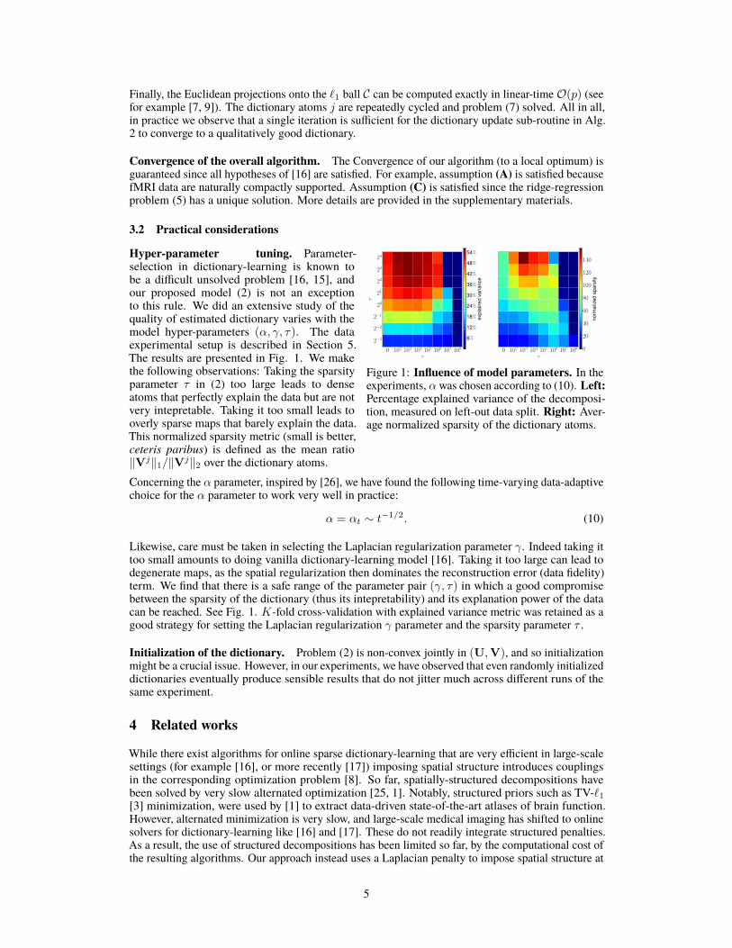
Figure 1: Influence of model parameters. In theexperiments, αwas chosen according to (10). Left:Percentage explained variance of the decomposi-tion, measured on left-out data split. Right: Aver-age normalized sparsity of the dictionary atoms.

Hyper-parameter tuning. Parameter-selection in dictionary-learning is known tobe a difficult unsolved problem [16, 15], andour proposed model (2) is not an exceptionto this rule. We did an extensive study of thequality of estimated dictionary varies with themodel hyper-parameters (α, γ, τ). The dataexperimental setup is described in Section 5.The results are presented in Fig. 1. We makethe following observations: Taking the sparsityparameter τ in (2) too large leads to denseatoms that perfectly explain the data but are notvery intepretable. Taking it too small leads tooverly sparse maps that barely explain the data.This normalized sparsity metric (small is better,ceteris paribus) is defined as the mean ratio‖Vj‖1/‖Vj‖2 over the dictionary atoms.Concerning the α parameter, inspired by [26], we have found the following time-varying data-adaptivechoice for the α parameter to work very well in practice:

α = αt ∼ t−1/2. (10)

Likewise, care must be taken in selecting the Laplacian regularization parameter γ. Indeed taking ittoo small amounts to doing vanilla dictionary-learning model [16]. Taking it too large can lead todegenerate maps, as the spatial regularization then dominates the reconstruction error (data fidelity)term. We find that there is a safe range of the parameter pair (γ, τ) in which a good compromisebetween the sparsity of the dictionary (thus its intepretability) and its explanation power of the datacan be reached. See Fig. 1. K-fold cross-validation with explained variance metric was retained as agood strategy for setting the Laplacian regularization γ parameter and the sparsity parameter τ .

Initialization of the dictionary. Problem (2) is non-convex jointly in (U,V), and so initializationmight be a crucial issue. However, in our experiments, we have observed that even randomly initializeddictionaries eventually produce sensible results that do not jitter much across different runs of thesame experiment.

4 Related works

While there exist algorithms for online sparse dictionary-learning that are very efficient in large-scalesettings (for example [16], or more recently [17]) imposing spatial structure introduces couplingsin the corresponding optimization problem [8]. So far, spatially-structured decompositions havebeen solved by very slow alternated optimization [25, 1]. Notably, structured priors such as TV-`1[3] minimization, were used by [1] to extract data-driven state-of-the-art atlases of brain function.However, alternated minimization is very slow, and large-scale medical imaging has shifted to onlinesolvers for dictionary-learning like [16] and [17]. These do not readily integrate structured penalties.As a result, the use of structured decompositions has been limited so far, by the computational cost ofthe resulting algorithms. Our approach instead uses a Laplacian penalty to impose spatial structure at

5

a very minor cost and adapts the online-learning dictionary-learning framework [16], resulting in afast and scalable structured decomposition. Second, the approach in [1] though very novel, is mostlyheuristic. In contrast, our method enjoys the same convergence guarantees and comparable numericalcomplexity as the basic unstructured online dictionary-learning [16].Finally, one should also mention [23] that introduced an online group-level functional brain mappingstrategy for differentiating regions reflecting the variety of brain network configurations observed in athe population, by learning a sparse-representation of these in the spirit of [16].

5 Experiments

Setup. Our experiments were done on task fMRI data from 500 subjects from the HCP –HumanConnectome Project– dataset [20]. These task fMRI data were acquired in an attempt to assessmajor domains that are thought to sample the diversity of neural systems of interest in functionalconnectomics. We studied the activation maps related to a task that involves language (story under-standing) and mathematics (mental computation). This particular task is expected to outline number,attentional and language networks, but the variability modes observed in the population cover evenwider cognitive systems. For the experiments, mass-univariate General Linear Models (GLMs) [10]for n = 500 subjects were estimated for the Math vs Story contrast (language protocol), and thecorresponding full-brain Z-score maps each containing p = 2.6× 105 voxels, were used as the inputdata X ∈ Rn×p, and we sought a decomposition into a dictionary of k = 40 atoms (components).The input data X were shuffled and then split into two groups of the same size.

Models compared and metrics. We compared our proposed Smooth-SODL model (2) againstboth the Canonical ICA –CanICA [22], a single-batch multi-subject PCA/ICA-based method, andthe standard SODL (sparse online dictionary-learning) [16]. While the CanICA model accounts forsubject-to-subject differences, one of its major limitations is that it does not model spatial variabilityacross subjects. Thus we estimated the CanICA components on smoothed data: isotropic FWHM of6mm, a necessary preprocessing step for such methods. In contrast, we did not perform pre-smoothingfor the SODL of Smooth-SODL models. The different models were compared across a variety ofqualitative and quantitative metrics: visual quality of the dictionaries obtained, explained variance,stability of the dictionary atoms, their reproducibility, performance of the dictionaries in predictingbehavioral scores (IQ, picture vocabulary, reading proficiency, etc.) shipped with the HCP data [20].For both SODL [16] and our proposed Smooth-SODL model, the constraint set for the dictionaryatoms was taken to be a simplex C := Sp(τ) (see section 2 for definition). The results of theseexperiments are presented in Fig. 2 and Tab. 1.

6 Results

Running time. On the computational side, the vanilla dictionary-learning SODL algorithm [16]with a batch size of η = 20 took about 110s (≈ 1.7 minutes) to run, whilst with the same batch size,our proposed Smooth-SODL model (2) implemented in Alg. 1 took 340s (≈ 5.6 minutes), whichis slightly less than 3 times slower than SODL. Finally, CanICA [22] for this experiment took 530s(≈ 8.8 minutes) to run, which is about 5 times slower than the SODL model and 1.6 times slowerthan our proposed Smooth-SODL (2) model. All experiments were run on a single CPU of laptop.

Qualitative assessment of dictionaries. As can be seen in Fig. 2(a), all methods recover dictionaryatoms that represent known functional brain organization; notably the dictionaries all contain thewell-known executive control and attention networks, at least in part. Vanilla dictionary-learningleverages the denoising properties of the `1 sparsity constraint, but the voxel clusters are not verystructured. For, example most blobs are surrounded with a thick ring of very small nonzero values. Incontrast, our proposed regularization model leverages both sparse and structured dictionary atoms,that are more spatially structured and less noisy.In contrast to both SODL and Smooth-SODL, CanICA [22] is an ICA-based method that enforces nonotion of sparsity whatsoever. The result are therefore dense and noisy dictionary atoms that explainthe data very well (Fig. 2(b) but which are completely unintepretable. In a futile attempt to remedythe situation, in practice such PCA/ICA-based methods (including FSL’s MELODIC tool [19]) arehard-thresholded in order to see information. For CanICA, the hard-thresholded version has been

6

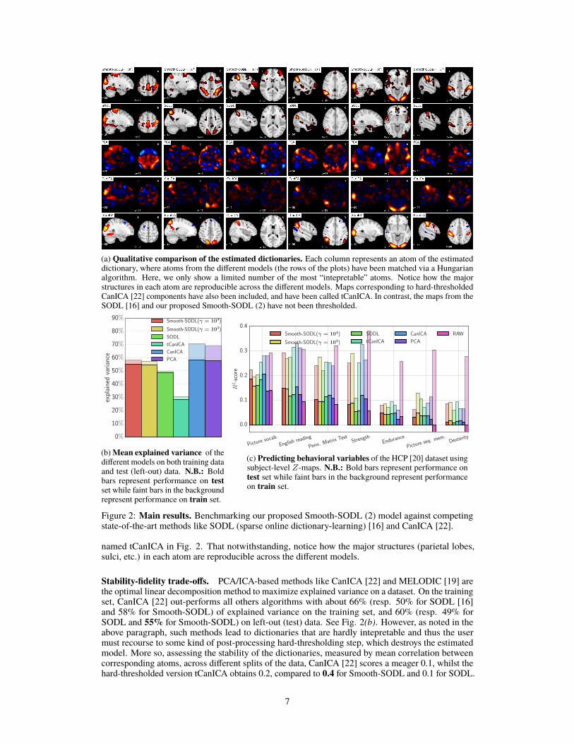
(a) Qualitative comparison of the estimated dictionaries. Each column represents an atom of the estimateddictionary, where atoms from the different models (the rows of the plots) have been matched via a Hungarianalgorithm. Here, we only show a limited number of the most “intepretable” atoms. Notice how the majorstructures in each atom are reproducible across the different models. Maps corresponding to hard-thresholdedCanICA [22] components have also been included, and have been called tCanICA. In contrast, the maps from theSODL [16] and our proposed Smooth-SODL (2) have not been thresholded.

0%

10%

20%

30%

40%

50%

60%

70%

80%

90%

expl

aine

dva

rian

ce

Smooth-SODL(γ = 104)

Smooth-SODL(γ = 103)

SODL

tCanICA

CanICA

PCA

(b)Mean explained variance of thedifferent models on both training dataand test (left-out) data. N.B.: Boldbars represent performance on testset while faint bars in the backgroundrepresent performance on train set.

Picture vocab.

English reading

Penn. Matrix TestStrength

Endurance

Picture seq. mem.Dexterity

0.0

0.1

0.2

0.3

0.4

R2-s

core

Smooth-SODL(γ = 104)

Smooth-SODL(γ = 103)

SODL

tCanICA

CanICA

PCA

RAW

(c) Predicting behavioral variables of the HCP [20] dataset usingsubject-level Z-maps. N.B.: Bold bars represent performance ontest set while faint bars in the background represent performanceon train set.

Figure 2: Main results. Benchmarking our proposed Smooth-SODL (2) model against competingstate-of-the-art methods like SODL (sparse online dictionary-learning) [16] and CanICA [22].

named tCanICA in Fig. 2. That notwithstanding, notice how the major structures (parietal lobes,sulci, etc.) in each atom are reproducible across the different models.

Stability-fidelity trade-offs. PCA/ICA-based methods like CanICA [22] and MELODIC [19] arethe optimal linear decomposition method to maximize explained variance on a dataset. On the trainingset, CanICA [22] out-performs all others algorithms with about 66% (resp. 50% for SODL [16]and 58% for Smooth-SODL) of explained variance on the training set, and 60% (resp. 49% forSODL and 55% for Smooth-SODL) on left-out (test) data. See Fig. 2(b). However, as noted in theabove paragraph, such methods lead to dictionaries that are hardly intepretable and thus the usermust recourse to some kind of post-processing hard-thresholding step, which destroys the estimatedmodel. More so, assessing the stability of the dictionaries, measured by mean correlation betweencorresponding atoms, across different splits of the data, CanICA [22] scores a meager 0.1, whilst thehard-thresholded version tCanICA obtains 0.2, compared to 0.4 for Smooth-SODL and 0.1 for SODL.

7

Is spatial regularization really needed ? As rightly pointed out by one of the reviewers, one doesnot need spatial regularization if data are abundant (like in the HCP). So we computed learning curvesof mean explained variance (EV) on test data, as a function of the amount training data seen byboth Smooth-SODL and SODL [16] (Table 1). In the beginning of the curve, our proposed spatiallyregularized Smooth-SODL model starts off with more than 31% explained variance (computed on241 subjects), after having pooled only 17 subjects. In contrast, the vanilla SODL model [16] scoresa meager 2% explained variance; this corresponds to a 14-fold gain of Smooth-SODL over SODL. Asmore and more data are pooled, both models explain more variance, the gap between Smooth-SODLand SODL reduces, and both models perform comparably asymptotically.

Nb. subjects pooled mean EV for vanilla SODL Smooth-SODL (2) gain factor17 2% 31% 13.892 37% 50% 1.35167 47% 54% 1.15241 49% 55% 1.11

Table 1: Learning-curve for boost in explained variance of our proposed Smooth-SODL model overthe reference SODL model. Note the reduction in the explained variance gain as more data are pooled.

Thus our proposed Smooth-SODL method extracts structured denoised dictionaries that better captureinter-subject variability in small, medium, and large-scale regimes alike.

Prediction of behavioral variables. If Smooth-SODL captures the patterns of inter-subject variabil-ity, then it should be possible to predict cognitive scores y like picture vocabulary, reading proficiency,math aptitude, etc. (the behavioral variables are explained in the HCP wiki [12]) by projecting newsubjects’ data into this learned low-dimensional space (via solving the ridge problem (5) for eachsample Xt), without loss of performance compared with using the raw Z-values values X. Let RAWrefer to the direct prediction of targets y fromX, using the top 2000 most voxels most correlated withthe target variable. Results of for the comparison are shown in Fig. 2(c). Only variables predictedwith a a positive mean (across the different methods and across subjects) R-score are reported. Wesee that the RAW model, as expected over-fits drastically, scoring an R2 of 0.3 on training data andonly 0.14 on test data. Overall, for this metric CanICA performs best than all the other models inpredicting the different behavioral variables on test data. However, our proposed Smooth-SODLmodel outperforms both SODL [16] and tCanICA, the thresholded version of CanICA.

7 Concluding remarks

To extract structured functionally discriminating patterns from massive brain data (i.e data-drivenatlases), we have extended the online dictionary-learning framework first developed in [16], to learnstructured regions representative of brain organization. To this end, we have successfully augmented[16] with a Laplacian penalty on the component maps, while conserving the low numerical complexityof the latter. Through experiments, we have shown that the resultant model –Smooth-SODLmodel (2)–extracts structured and denoised dictionaries that are more intepretable and better capture inter-subjectvariability in small medium, and large-scale regimes alike, compared to state-of-the-art models. Webelieve such online multivariate online methods shall become the de facto way to do dimensionalityreduction and ROI extraction in the future.

Implementation. The authors’ implementation of the proposed Smooth-SODL (2) model will soonbe made available as part of the Nilearn package [2].

Acknowledgment. This work has been funded by EU FP7/2007-2013 under grant agreement no.604102, Human Brain Project (HBP) and the iConnectome Digiteo. We would also like to thank theHuman Connectome Projection for making their wonderful data publicly available.

8

References

[1] A. Abraham et al. “Extracting brain regions from rest fMRI with Total-Variation constraineddictionary learning”. In: MICCAI. 2013.

[2] A. Abraham et al. “Machine learning for neuroimaging with scikit-learn”. In: Frontiers inNeuroinformatics (2014).

[3] L. Baldassarre, J. Mourao-Miranda, and M. Pontil. “Structured sparsity models for braindecoding from fMRI data”. In: PRNI. 2012.

[4] A. Beck and M. Teboulle. “A Fast Iterative Shrinkage-Thresholding Algorithm for LinearInverse Problems”. In: SIAM J. Imaging Sci. 2 (2009).

[5] C. F. Beckmann and S. M. Smith. “Probabilistic independent component analysis for functionalmagnetic resonance imaging”. In: Trans Med. Im. 23 (2004).

[6] D. P. Bertsekas. Nonlinear programming. Athena Scientific, 1999.[7] L. Condat. “Fast projection onto the simplex and the `1 ball”. In: Math. Program. (2014).[8] E. Dohmatob et al. “Benchmarking solvers for TV-l1 least-squares and logistic regression in

brain imaging”. In: PRNI. IEEE. 2014.[9] J. Duchi et al. “Efficient projections onto the l 1-ball for learning in high dimensions”. In:

ICML. ACM. 2008.[10] K. J. Friston et al. “Statistical Parametric Maps in Functional Imaging: A General Linear

Approach”. In: Hum Brain Mapp (1995).[11] L. Grosenick et al. “Interpretable whole-brain prediction analysis with GraphNet”. In: Neu-

roImage 72 (2013).[12] HCP wiki. https://wiki.humanconnectome.org/display/PublicData/HCP+Data+

Dictionary+Public-+500+Subject+Release. Accessed: 2010-09-30.[13] M. Hebiri and S. van de Geer. “The Smooth-Lasso and other `1 + `2-penalized methods”. In:

Electron. J. Stat. 5 (2011).[14] D. P. Hibar et al. “Genetic clustering on the hippocampal surface for genome-wide association

studies”. In: MICCAI. 2013.[15] R. Jenatton, G. Obozinski, and F. Bach. “Structured sparse principal component analysis”. In:

AISTATS. 2010.[16] J. Mairal et al. “Online learning for matrix factorization and sparse coding”. In: Journal of

Machine Learning Research 11 (2010).[17] A. Mensch et al. “Dictionary Learning for Massive Matrix Factorization”. In: ICML. ACM.

2016.[18] R. Saxe, M. Brett, and N. Kanwisher. “Divide and conquer: a defense of functional localizers”.

In: Neuroimage 30 (2006).[19] S.M. Smith et al. “Advances in functional and structuralMR image analysis and implementation

as FSL”. In: Neuroimage 23 (2004).[20] D. van Essen et al. “The Human Connectome Project: A data acquisition perspective”. In:

NeuroImage 62 (2012).[21] E. Varol and C. Davatzikos. “Supervised block sparse dictionary learning for simultaneous

clustering and classification in computational anatomy.” eng. In: Med Image Comput ComputAssist Interv 17 (2014).

[22] G. Varoquaux et al. “A group model for stable multi-subject ICA on fMRI datasets”. In:Neuroimage 51 (2010).

[23] G. Varoquaux et al. “Cohort-level brain mapping: learning cognitive atoms to single outspecialized regions”. In: IPMI. 2013.

[24] G. Varoquaux et al. “FAASTA: A fast solver for total-variation regularization of ill-conditionedproblems with application to brain imaging”. In: arXiv:1512.06999 (2015).

[25] G. Varoquaux et al. “Multi-subject dictionary learning to segment an atlas of brain spontaneousactivity”. In: Inf Proc Med Imag. 2011.

[26] Y. Ying and D.-X. Zhou. “Online regularized classification algorithms”. In: IEEE Trans. Inf.Theory 52 (2006).

9