© Wiley 2010

Chapter 6 - Statistical Quality Control

Operations Managementby

R. Dan Reid & Nada R. Sanders4th Edition © Wiley 2010

PowerPoint Presentation by R.B. Clough – UNHM. E. Henrie - UAA

© Wiley 2010

Three SQC Categories Statistical quality control (SQC) is the term used to

describe the set of statistical tools used by quality professionals

SQC encompasses three broad categories of; Descriptive statistics

e.g. the mean, standard deviation, and range Statistical process control (SPC)

Involves inspecting the output from a process Quality characteristics are measured and charted Helpful in identifying in-process variations

Acceptance sampling used to randomly inspect a batch of goods to determine acceptance/rejection

Does not help to catch in-process problems

© Wiley 2010

Sources of Variation Variation exists in all processes. Variation can be categorized as either;

Common or Random causes of variation, or Random causes that we cannot identify Unavoidable e.g. slight differences in process variables like diameter,

weight, service time, temperature

Assignable causes of variation Causes can be identified and eliminated e.g. poor employee training, worn tool, machine needing repair

© Wiley 2010

Traditional Statistical Tools Descriptive Statistics

include The Mean- measure of

central tendency

The Range- difference between largest/smallest observations in a set of data

Standard Deviation measures the amount of data dispersion around mean

Distribution of Data shape Normal or bell shaped or Skewed

n

xx

n

1ii

1n

Xxσ

n

1i

2

i

© Wiley 2010

Distribution of Data Normal

distributions

Skewed distribution

© Wiley 2010

SPC Methods-Control Charts

Control Charts show sample data plotted on a graph with CL, UCL, and LCL

Control chart for variables are used to monitor characteristics that can be measured, e.g. length, weight, diameter, time

Control charts for attributes are used to monitor characteristics that have discrete values and can be counted, e.g. % defective, number of flaws in a shirt, number of broken eggs in a box

© Wiley 2010

Setting Control Limits Percentage of values

under normal curve

Control limits balance

risks like Type I error

© Wiley 2010

Control Charts for Variables

Use x-bar and R-bar charts together

Used to monitor different variables

X-bar & R-bar Charts reveal different problems

In statistical control on one chart, out of control on the other chart? OK?

© Wiley 2010

Control Charts for Variables Use x-bar charts to monitor the

changes in the mean of a process (central tendencies)

Use R-bar charts to monitor the dispersion or variability of the process

System can show acceptable central tendencies but unacceptable variability or

System can show acceptable variability but unacceptable central tendencies

© Wiley 2010

Constructing a X-bar Chart: A quality control inspector at the Cocoa Fizz soft drink company has taken three samples with four observations each of the volume of bottles filled. If the standard deviation of the bottling operation is .2 ounces, use the below data to develop control charts with limits of 3 standard deviations for the 16 oz. bottling operation.

Center line and control limit formulas

xx

xx

n21

zσxLCL

zσxUCL

sample each w/in nsobservatio of# the is

(n) and means sample of # the is )( wheren

σσ ,

...xxxx x

k

k

observ 1 observ 2 observ 3 observ 4 mean rangesamp 1 15.8 16 15.8 15.9 15.88 0.2samp 2 16.1 16 15.8 15.9 15.95 0.3samp 3 16 15.9 15.9 15.8 15.90 0.2

© Wiley 2010

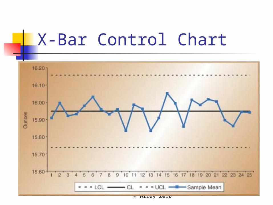
Solution and Control Chart (x-bar)

Center line (x-double bar):

Control limits for±3σ limits:

15.923

15.915.97515.875x

15.624

.2315.92zσxLCL

16.224

.2315.92zσxUCL

xx

xx

© Wiley 2010

X-Bar Control Chart

© Wiley 2010

Control Chart for Range (R)

Center Line and Control Limit formulas:

Factors for three sigma control limits

0.00.0(.233)RDLCL

.532.28(.233)RDUCL

.2333

0.20.30.2R

3

4

R

R

Factor for x-Chart

A2 D3 D42 1.88 0.00 3.273 1.02 0.00 2.574 0.73 0.00 2.285 0.58 0.00 2.116 0.48 0.00 2.007 0.42 0.08 1.928 0.37 0.14 1.869 0.34 0.18 1.8210 0.31 0.22 1.7811 0.29 0.26 1.7412 0.27 0.28 1.7213 0.25 0.31 1.6914 0.24 0.33 1.6715 0.22 0.35 1.65

Factors for R-ChartSample Size (n)

© Wiley 2010

R-Bar Control Chart

© Wiley 2010

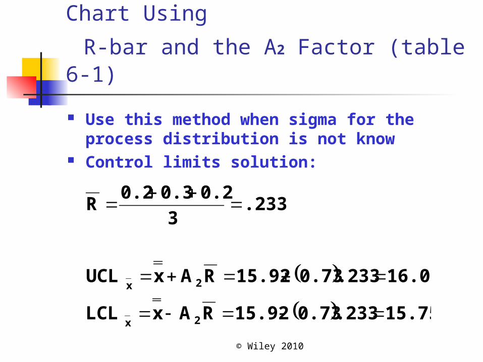
Second Method for the X-bar Chart Using

R-bar and the A2 Factor (table 6-1)

Use this method when sigma for the process distribution is not know

Control limits solution:

15.75.2330.7315.92RAxLCL

16.09.2330.7315.92RAxUCL

.2333

0.20.30.2R

2x

2x

© Wiley 2010

Control Charts for Attributes i.e. discrete events

Use a P-Chart for yes/no or good/bad decisions in which defective items are clearly identified

Use a C-Chart for more general counting when there can be more than one defect per unit

Number of flaws or stains in a carpet sample cut from a production run

Number of complaints per customer at a hotel

© Wiley 2010

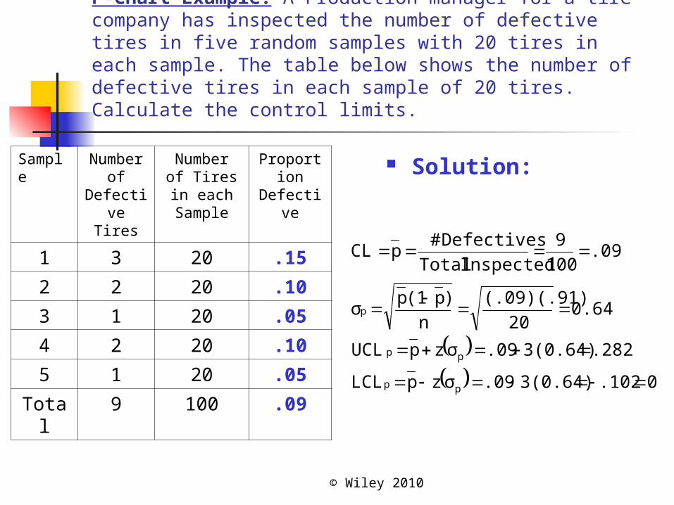
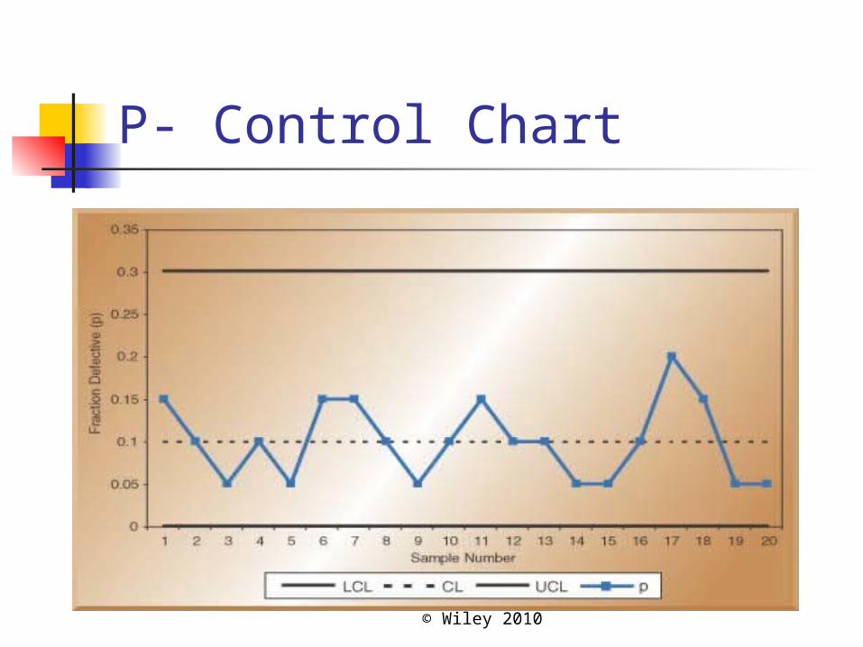
P-Chart Example: A Production manager for a tire company has inspected the number of defective tires in five random samples with 20 tires in each sample. The table below shows the number of defective tires in each sample of 20 tires. Calculate the control limits.

Sample

Number of

Defective Tires

Number of Tires in each

Sample

Proportion

Defective

1 3 20 .15

2 2 20 .10

3 1 20 .05

4 2 20 .10

5 1 20 .05

Total 9 100 .09

Solution:

0.1023(0.64).09σzpLCL

.2823(0.64).09σzpUCL

0.6420

(.09)(.91)

n

)p(1pσ

.09100

9

Inspected Total

Defectives#pCL

pp

pp

p

© Wiley 2010

P- Control Chart

© Wiley 2010

C-Chart Example: The number of weekly customer complaints are monitored in a large hotel using a c-chart. Develop three sigma control limits using the data table below.

Week Number of Complaints

1 3

2 2

3 3

4 1

5 3

6 3

7 2

8 1

9 3

10 1

Total 22

Solution:

02.252.232.2ccLCL

6.652.232.2ccUCL

2.210

22

samples of #

complaints#cCL

c

c

z

z

© Wiley 2010

C- Control Chart

© Wiley 2010

Out of control conditions indicated by:

Skewed distributionData Point out of limits

© Wiley 2010

Process Capability Product Specifications

Preset product or service dimensions, tolerances e.g. bottle fill might be 16 oz. ±.2 oz. (15.8oz.-16.2oz.) Based on how product is to be used or what the customer expects

Process Capability – Cp and Cpk Assessing capability involves evaluating process variability

relative to preset product or service specifications Cp assumes that the process is centered in the specification range

Cpk helps to address a possible lack of centering of the process

6σ

LSLUSL

width process

width ionspecificatCp

3σ

LSLμ,

3σ

μUSLminCpk

© Wiley 2010

Relationship between Process Variability and Specification Width

Possible ranges for Cp

Cp < 1, as in Fig. (b), process not capable of producing within specifications

Cp ≥ 1, as in Fig. (c), process exceeds minimal

specifications

One shortcoming, Cp assumes that the process is centered on the specification range

Cp=Cpk when process is centered

© Wiley 2010

Computing the Cp Value at Cocoa Fizz: three bottling machines are being evaluated for possible use at the Fizz plant. The machines must be capable of meeting the design specification of 15.8-16.2 oz. with at least a process capability index of 1.0 (Cp≥1)

The table below shows the information gathered from production runs on each machine. Are they all acceptable?

Solution: Machine A

Machine B

Machine C

Machine

σ USL-LSL

6σ

A .05 .4 .3

B .1 .4 .6

C .2 .4 1.2

1.336(.05)

.4

6σ

LSLUSLCp

67.06(.1)

.4

6σ

LSLUSLCp

0.336(.2)

.4

6σ

LSLUSLCp

© Wiley 2010

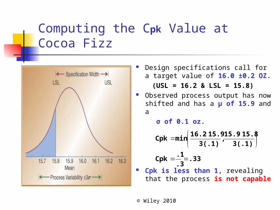
Computing the Cpk Value at Cocoa Fizz

Design specifications call for a target value of 16.0 ±0.2 OZ.

(USL = 16.2 & LSL = 15.8) Observed process output has

now shifted and has a µ of 15.9 and a

σ of 0.1 oz.

Cpk is less than 1, revealing that the process is not capable

.33.3

.1Cpk

3(.1)

15.815.9,

3(.1)

15.916.2minCpk

© Wiley 2010

±6 Sigma versus ± 3 Sigma

Motorola coined “six-sigma” to describe their higher quality efforts back in 1980’s

Ordinary quality standard requiring mean±3σ to be within tolerances implies that 99.74% of production is between LSL and USL

Six sigma is much stricter: mean ±6σ must be within tolerances implying that 99.99966% production between LSL and USL

same proportions apply to control limits in control charts

Six-sigma quality standard is now a benchmark in many industries

PPM Defective for ±3σ versus ±6σ quality

© Wiley 2010

Six SigmaSix Sigma Still Pays Off At Motorola

It may surprise those who have come to know Motorola (MOT ) for its cool cell phones, but the company's more lasting contribution to the world is something decidedly more wonkish: the quality-improvement process called Six Sigma. In 1986 an engineer named Bill Smith, who has since died, sold then-Chief Executive Robert Galvin on a plan to strive for error-free products 99.9997% of the time. By Six Sigma's 20th anniversary, the exacting, metrics-driven process has become corporate gospel, infiltrating functions from human resources to marketing, and industries from manufacturing to financial services.

Others agree that Six Sigma and innovation don't have to be a cultural mismatch. At Nortel Networks (NT ), CEO Mike S. Zafirovski, a veteran of both Motorola and Six Sigma stalwart General Electric (GE ) Co., has installed his own version of the program, one that marries concepts from Toyota Motor (TM )'s lean production system. The point, says Joel Hackney, Nortel's Six Sigma guru, is to use Six Sigma thinking to take superfluous steps out of operations. Running a more efficient shop, he argues, will free up workers to innovate.

http://www.businessweek.com/magazine/content/06_49/b4012069.htm?chan=search

© Wiley 2010

Acceptance Sampling Definition: the third branch of SQC refers to the

process of randomly inspecting a certain number of items from a lot or batch in order to decide whether to accept or reject the entire batch

Different from SPC because acceptance sampling is performed either before or after the process rather than during

Sampling before typically is done to supplier material Sampling after involves sampling finished items before

shipment or finished components prior to assembly Used where inspection is expensive, volume is

high, or inspection is destructive

© Wiley 2010

Acceptance Sampling Plans Goal of Acceptance Sampling plans is to determine the

criteria for acceptance or rejection based on: Size of the lot (N)

Size of the sample (n)

Number of defects above which a lot will be rejected (c)

Level of confidence we wish to attain

There are single, double, and multiple sampling plans Which one to use is based on cost involved, time consumed, and

cost of passing on a defective item

Can be used on either variable or attribute measures,

but more commonly used for attributes

© Wiley 2010

Implications for Managers How much and how often to inspect?

Consider product cost and product volume Consider process stability Consider lot size

Where to inspect? Inbound materials Finished products Prior to costly processing

Which tools to use? Control charts are best used for in-process production Acceptance sampling is best used for

inbound/outbound

© Wiley 2010

SQC in Services Service Organizations have lagged behind

manufacturers in the use of statistical quality control Statistical measurements are required and it is more

difficult to measure the quality of a service Services produce more intangible products Perceptions of quality are highly subjective

A way to deal with service quality is to devise quantifiable measurements of the service element

Check-in time at a hotel Number of complaints received per month at a restaurant Number of telephone rings before a call is answered Acceptable control limits can be developed and charted

© Wiley 2010

Service at a bank: The Dollars Bank competes on customer service and is concerned about service time at their drive-by windows. They recently installed new system software which they hope will meet service specification limits of 5±2 minutes and have a Capability Index (Cpk) of at least 1.2. They want to also design a control chart for bank teller use.

They have done some sampling recently (sample size of 4 customers) and determined that the process mean has shifted to 5.2 with a Sigma of 1.0 minutes.

Control Chart limits for ±3 sigma limits

1.21.5

1.8Cpk

3(1/2)

5.27.0,

3(1/2)

3.05.2minCpk

1.33

4

1.06

3-7

6σ

LSLUSLCp

minutes 6.51.55.04

135.0zσXUCL xx

minutes 3.51.55.04

135.0zσXLCL xx

© Wiley 2010

SQC Across the Organization SQC requires input from other organizational

functions, influences their success, and are actually used in designing and evaluating their tasks

Marketing – provides information on current and future quality standards

Finance – responsible for placing financial values on SQC efforts

Human resources – the role of workers change with SQC implementation. Requires workers with right skills

Information systems – makes SQC information accessible for all.

© Wiley 2010

There’s $$ is SQC!

“I also discovered that the work I had done for Motorola in my first year out of college had a name. I was doing Operations Management, by measuring service quality for paging by using statistical process control methods.”

-Michele Davies, Businessweek MBA Journals, May 2001http://www.businessweek.com/bschools/mbajournal/00davies/6.htm?chan=search

© Wiley 2010

..and Long Life?

http://www.businessweek.com/magazine/content/04_35/b3897017_mz072.htm?chan=searchhttp://www.businessweek.com/magazine/content/04_35/b3897017_mz072.htm?chan=search

© Wiley 2010

Chapter 6 Highlights SQC refers to statistical tools t hat can be sued by

quality professionals. SQC an be divided into three categories: traditional statistical tools, acceptance sampling, and statistical process control (SPC).

Descriptive statistics are sued to describe quality characteristics, such as the mean, range, and variance. Acceptance sampling is the process of randomly inspecting a sample of goods and deciding whether to accept or reject the entire lot. Statistical process control involves inspecting a random sample of output from a process and deciding whether the process in producing products with characteristics that fall within preset specifications.

© Wiley 2010

Chapter 6 Highlights - continued

Two causes of variation in the quality of a product or process: common causes and assignable causes. Common causes of variation are random causes that we cannot identify. Assignable causes of variation are those that can be identified and eliminated.

A control chart is a graph used in SPC that shows whether a sample of data falls within the normal range of variation. A control chart has upper and lower control limits that separate common from assignable causes of variation. Control charts for variables monitor characteristics that can be measured and have a continuum of values, such as height, weight, or volume. Control charts fro attributes are used to monitor characteristics that have discrete values and can be counted.

© Wiley 2010

Chapter 6 Highlights - continued

Control charts for variables include x-bar and R-charts. X-bar charts monitor the mean or average value of a product characteristic. R-charts monitor the range or dispersion of the values of a product characteristic. Control charts for attributes include p-charts and c-charts. P-charts are used to monitor the proportion of defects in a sample, C-charts are used to monitor the actual number of defects in a sample.

Process capability is the ability of the production process to meet or exceed preset specifications. It is measured by the process capability index Cp which is computed as the ratio of the specification width to the width of the process variable.

© Wiley 2010

Chapter 6 Highlights - continued

The term Six Sigma indicates a level of quality in which the number of defects is no more than 2.3 parts per million.

The goal of acceptance sampling is to determine criteria for the desired level of confidence. Operating characteristic curves are graphs that show the discriminating power of a sampling plan.

It is more difficult to measure quality in services than in manufacturing. The key is to devise quantifiable measurements for important service dimensions.

© Wiley 2010

The End Copyright © 2010 John Wiley & Sons, Inc. All rights

reserved. Reproduction or translation of this work beyond that permitted in Section 117 of the 1976 United State Copyright Act without the express written permission of the copyright owner is unlawful. Request for further information should be addressed to the Permissions Department, John Wiley & Sons, Inc. The purchaser may make back-up copies for his/her own use only and not for distribution or resale. The Publisher assumes no responsibility for errors, omissions, or damages, caused by the use of these programs or from the use of the information contained herein.