tesi sullo streaming in p2p
DESCRIPTION
Tesi sullo Streaming in P2P, pubblicata dall'autore del software GoalbitTRANSCRIPT
No d’ordre: 00000
THÈSE
présentée
devant l’Université de Rennes 1
pour obtenir
le grade de : DOCTEUR DE L’UNIVERSITÉ DE RENNES 1Mention INFORMATIQUE
par
Pablo RODRÍGUEZ-BOCCA
Équipe d’accueil : DIONYSOS - IRISAÉcole Doctorale : Matisse
Composante universitaire : IFSIC
Titre de la thèse :
Quality-centric design of Peer-to-Peer systemsfor live-video broadcasting
À soutenir le 28 février 2008 devant la commission d’examen
M. : Alberto PARDO PrésidentMM. : Edmundo DE SOUZA E SILVA Rapporteurs
Fernando PAGANINI
MM. : Eduardo GRAMPIN ExaminateursDaniel KOFMAN
César VIHO
MM. : Héctor CANCELA Directeurs de thèseGerardo RUBINO


Remerciements
Je remercie Alberto PARDO, Professeur, Universidad de la República, Uruguay, qui me faitl’honneur de présider ce jury.
Je remercie Edmundo DE SOUZA E SILVA, Professeur, Federal University of Rio de Janeiro,COPPE/ Computer Science Department, et Fernando PAGANINI, Professeur, Universidad ORT,Uruguay, d’avoir bien voulu accepter la charge de rapporteur.
Je remercie Eduardo GRAMPIN, Professeur, Universidad de la República, Uruguay, DanielKOFMAN, Professeur, ENST/INFRES/RHD, et César VIHO, Professeur, INRIA Rennes, d’avoirbien voulu juger ce travail.
Je remercie tous les membres du projet GOL!P2P qui m’ont fourni un appui indispensablependant la réalisatino de cette thèse, et je remercie spécialement Héctor CANCELA, Professeur,Universidad de la República, Uruguay, et Gerardo RUBINO, Directeur de Recherche, INRIARennes, qui ont dirigé ma thèse.


Contents
Table des matières 1
I INTRODUCTION 7
1 Global presentation of the thesis 91.1 Motivation and goals . . . . . . . . . . . . . . . . . . . . . . . . . . . . . . . 91.2 Contributions . . . . . . . . . . . . . . . . . . . . . . . . . . . . . . . . . . . 10
1.2.1 Quality of Experience . . . . . . . . . . . . . . . . . . . . . . . . . . 111.2.2 Multi-source Distribution using a P2P Approach . . . . . . . . . . . . 111.2.3 Efficient Search in Video Libraries . . . . . . . . . . . . . . . . . . . . 121.2.4 Quality-driven Dynamic Control of Video Delivery Networks . . . . . 12
1.3 Document Outline . . . . . . . . . . . . . . . . . . . . . . . . . . . . . . . . . 131.4 Publications . . . . . . . . . . . . . . . . . . . . . . . . . . . . . . . . . . . . 15
2 Background 192.1 Digital Video Overview. . . . . . . . . . . . . . . . . . . . . . . . . . . . . . 19
2.1.1 Compression and Standard Coding of digital video . . . . . . . . . . . 192.1.2 Digital video applications and Streaming Issues . . . . . . . . . . . . . 21
2.2 Video Delivery Networks . . . . . . . . . . . . . . . . . . . . . . . . . . . . . 222.2.1 A Simple Network Model. . . . . . . . . . . . . . . . . . . . . . . . . 222.2.2 Quality-of-Experience (QoE) in a VDN. . . . . . . . . . . . . . . . . . 252.2.3 Summary . . . . . . . . . . . . . . . . . . . . . . . . . . . . . . . . . 26
2.3 Peer-to-Peer Network Architecture for Video Delivery on Internet . . . . . . . 282.3.1 Introduction, the Content Networks . . . . . . . . . . . . . . . . . . . 282.3.2 Content Networks for Video Delivery on Internet . . . . . . . . . . . . 30
2.3.2.1 Scale and Cost Problem of Live-video Delivery on Internet . 302.3.2.2 Content Delivery Networks (CDN): global scalability . . . . 312.3.2.3 Peer-to-Peer Networks (P2P): cutting off the costs . . . . . . 33
2.3.3 Peer-to-Peer (P2P) Networks . . . . . . . . . . . . . . . . . . . . . . . 332.3.3.1 Overlay Network: the control and routing layer . . . . . . . 342.3.3.2 Structured Overlays for Live Video Streaming . . . . . . . . 362.3.3.3 Content Delivery: the data download from the client point of
view . . . . . . . . . . . . . . . . . . . . . . . . . . . . . . 41
1

2 Contents
2.3.4 Introduction to Network Robustness: an hybrid P2P approach . . . . . 422.3.5 Summary: Conclusions, Results and Discussion . . . . . . . . . . . . . 43
2.4 Search Caching: an approach for discovery scalability in Content Networks . . 432.5 A Video Delivery Reference Service . . . . . . . . . . . . . . . . . . . . . . . 442.6 Summary . . . . . . . . . . . . . . . . . . . . . . . . . . . . . . . . . . . . . 47
II QUALITY 49
3 Video Quality Assessment: State of the art 513.1 Subjective Quality Assessment . . . . . . . . . . . . . . . . . . . . . . . . . . 51
3.1.1 Single Stimulus (SS) . . . . . . . . . . . . . . . . . . . . . . . . . . . 523.1.2 Double Stimulus Impairment Scale (DSIS) . . . . . . . . . . . . . . . 533.1.3 Double Stimulus Continuous Quality Scale (DSCQS) . . . . . . . . . . 543.1.4 Other Works in Subjective Video Quality Measures . . . . . . . . . . . 543.1.5 Subjective Test Comparison . . . . . . . . . . . . . . . . . . . . . . . 55
3.2 Objective Quality Assessment . . . . . . . . . . . . . . . . . . . . . . . . . . 563.2.1 Peak Signal–to–Noise Ratio (PSNR) . . . . . . . . . . . . . . . . . . . 573.2.2 ITS’ Video Quality Metric (VQM) . . . . . . . . . . . . . . . . . . . . 573.2.3 Moving Picture Quality Metric (MPQM) and Color Moving Picture
Quality Metric (CMPQM) . . . . . . . . . . . . . . . . . . . . . . . . 573.2.4 Normalization Video Fidelity Metric (NVFM) . . . . . . . . . . . . . . 583.2.5 Other Works in Objective Video Quality Measures and Comparison . . 58
3.3 An Hybrid Quality Assessment approach: Pseudo-Subjective Quality Assessment 593.4 Summary . . . . . . . . . . . . . . . . . . . . . . . . . . . . . . . . . . . . . 60
4 PSQA – Pseudo–Subjective Quality Assessment 634.1 Overview of the PSQA Methodology . . . . . . . . . . . . . . . . . . . . . . . 634.2 A Formal Notation . . . . . . . . . . . . . . . . . . . . . . . . . . . . . . . . 654.3 Stage I: Quality–affecting factors and Distorted Video Database Generation . . 65
4.3.1 Quality–affecting Parameters Selection . . . . . . . . . . . . . . . . . 664.3.2 Distorted Video Database Generation and Testbed Development . . . . 69
4.4 Stage II: Subjective Quality Assessment . . . . . . . . . . . . . . . . . . . . . 694.4.1 A Subjective Test Campaign . . . . . . . . . . . . . . . . . . . . . . . 704.4.2 Mean Opinion Score (MOS) Calculation and Related Statistical Analysis 70
4.5 Stage III: Learning of the quality behavior with a Random Neural Networks(RNN) 724.5.1 Random Neural Networks (RNN) overview . . . . . . . . . . . . . . . 724.5.2 Using RNN as a function approximator: a learning tool . . . . . . . . . 74
4.5.2.1 Training and Validating . . . . . . . . . . . . . . . . . . . . 754.5.3 The RNN topology design . . . . . . . . . . . . . . . . . . . . . . . . 75
4.5.3.1 The simplest design: a Two–Layer RNN Topology . . . . . . 764.5.3.2 The Three–Layer RNN Topology . . . . . . . . . . . . . . . 78
4.6 Operation Mode . . . . . . . . . . . . . . . . . . . . . . . . . . . . . . . . . . 804.7 Summary . . . . . . . . . . . . . . . . . . . . . . . . . . . . . . . . . . . . . 80

Contents 3
5 Studying the Effects of Several Parameters on the Perceived Video Quality 815.1 Parameters Selection: Network level or Application level? . . . . . . . . . . . 81
5.1.1 Packet and Frame Losses Correlation . . . . . . . . . . . . . . . . . . 825.2 Network and Server Failures Effect . . . . . . . . . . . . . . . . . . . . . . . . 84
5.2.1 Loss Rate and Mean Loss Burst Size . . . . . . . . . . . . . . . . . . . 845.2.1.1 Emulating the Losses in the Testbed: the simplified Gilbert
model . . . . . . . . . . . . . . . . . . . . . . . . . . . . . 845.2.2 Experiment Description . . . . . . . . . . . . . . . . . . . . . . . . . 865.2.3 PSQA Simple Function . . . . . . . . . . . . . . . . . . . . . . . . . . 875.2.4 PSQA Minimal Closed–form Function . . . . . . . . . . . . . . . . . . 89
5.3 Adding Video Source Motion Effect . . . . . . . . . . . . . . . . . . . . . . . 905.3.1 Quality-affecting parameters . . . . . . . . . . . . . . . . . . . . . . . 915.3.2 Experiment Description . . . . . . . . . . . . . . . . . . . . . . . . . 925.3.3 PSQA Complex Function . . . . . . . . . . . . . . . . . . . . . . . . . 93
5.4 Summary and Conclusions . . . . . . . . . . . . . . . . . . . . . . . . . . . . 96
III PEER-TO-PEER 99
6 Multi-Source Streaming Technique 1016.1 Introduction to multi-source streaming . . . . . . . . . . . . . . . . . . . . . . 101
6.1.1 Simple extreme multi-source methods: single, copied and splitted flows 1026.1.2 Related multi-source strategies . . . . . . . . . . . . . . . . . . . . . . 105
6.2 Utility of multi–source streaming techniques: Its impacts on Quality . . . . . . 1066.2.1 Multi-source Streaming Models . . . . . . . . . . . . . . . . . . . . . 107
6.2.1.1 Streaming from a single source . . . . . . . . . . . . . . . . 1076.2.1.2 Sending K copies of the stream . . . . . . . . . . . . . . . . 1076.2.1.3 Complete split of the stream into K ≥ 2 sub-streams . . . . 108
6.2.2 Evaluating and first results . . . . . . . . . . . . . . . . . . . . . . . . 1106.3 Summary and Conclusions . . . . . . . . . . . . . . . . . . . . . . . . . . . . 112
7 Optimal Quality in Multi-Source Streaming 1137.1 Video Quality Assurance: introducing the peers behavior . . . . . . . . . . . . 113
7.1.1 P2P Network and Dynamics Model . . . . . . . . . . . . . . . . . . . 1147.1.2 Multi-source Streaming Models . . . . . . . . . . . . . . . . . . . . . 115
7.1.2.1 Sending K copies of the stream . . . . . . . . . . . . . . . . 1157.1.2.2 Simple split of the stream into K ≥ 2 substreams . . . . . . 1167.1.2.3 Split of the stream into K ≥ 2 substreams, adding complete
redundancy . . . . . . . . . . . . . . . . . . . . . . . . . . 1177.1.3 Perceived Quality Evaluations and Results . . . . . . . . . . . . . . . . 117
7.1.3.1 Assuring Video Quality . . . . . . . . . . . . . . . . . . . . 1197.2 Improving the Multi-Source Streaming and Looking for Optimality: Consider-
ing the peers’ heterogeneity . . . . . . . . . . . . . . . . . . . . . . . . . . . . 1237.2.1 First improvement of the scheme: unequal splitting . . . . . . . . . . . 124
4 Contents
7.2.2 Improving the model of the peers’ dynamics . . . . . . . . . . . . . . 1247.2.3 Second improvement to the transmission method: discrimination per
frame type . . . . . . . . . . . . . . . . . . . . . . . . . . . . . . . . 1257.2.4 Optimization Results . . . . . . . . . . . . . . . . . . . . . . . . . . . 126
7.3 Assuring Quality at the Receiver: buffering protection . . . . . . . . . . . . . . 1307.3.1 Buffering Model . . . . . . . . . . . . . . . . . . . . . . . . . . . . . 1307.3.2 Buffering Protection Strategy . . . . . . . . . . . . . . . . . . . . . . 132
7.4 Summary and Conclusions . . . . . . . . . . . . . . . . . . . . . . . . . . . . 135
8 Structured Overlay Peer-to-Peer based on Quality Guarantees 1378.1 Background Definitions . . . . . . . . . . . . . . . . . . . . . . . . . . . . . . 1378.2 P2P Robust Assignment Model . . . . . . . . . . . . . . . . . . . . . . . . . . 1388.3 Looking for a Solution . . . . . . . . . . . . . . . . . . . . . . . . . . . . . . 140
8.3.1 Greedy heuristic solution . . . . . . . . . . . . . . . . . . . . . . . . . 1428.3.1.1 Enhancement criteria of a given assignment . . . . . . . . . 143
8.3.2 Algorithmic solution based on GRASP . . . . . . . . . . . . . . . . . 1448.3.2.1 Construction phase . . . . . . . . . . . . . . . . . . . . . . 1448.3.2.2 Local search phase . . . . . . . . . . . . . . . . . . . . . . . 145
8.3.3 GRASP improvement using RNN . . . . . . . . . . . . . . . . . . . . 1458.4 Preliminary performance estimation in a hybrid CDN-P2P structured network . 148
8.4.1 Generation of realistic test cases . . . . . . . . . . . . . . . . . . . . . 1488.4.2 Algorithms calibration . . . . . . . . . . . . . . . . . . . . . . . . . . 152
8.4.2.1 Restricted Candidate List (RCL) . . . . . . . . . . . . . . . 1528.4.2.2 RNN use percentage (rnn) in the RNN-improved GRASP . . 1538.4.2.3 Selection of the enhancement criteria of a given assignment:
“current” and “future” perceived quality . . . . . . . . . . . 1548.4.3 Comparing the performance of our algorithms: Greedy, GRASP and
GRASP+RNN . . . . . . . . . . . . . . . . . . . . . . . . . . . . . . 1558.4.4 Extending our Video Delivery Reference Service with a P2PTV system 156
8.5 Summary and Conclusions . . . . . . . . . . . . . . . . . . . . . . . . . . . . 157
IV CHALLENGES IN THE REALITY 159
9 Measure and Monitor the Quality of Real Video Services. 1619.1 Introduction . . . . . . . . . . . . . . . . . . . . . . . . . . . . . . . . . . . . 1619.2 Methodological Considerations . . . . . . . . . . . . . . . . . . . . . . . . . . 162
9.2.1 Simple Network Management Protocol . . . . . . . . . . . . . . . . . 1639.2.2 Quality Measurements. . . . . . . . . . . . . . . . . . . . . . . . . . 1639.2.3 An Extensible Measurement Framework. . . . . . . . . . . . . . . . . 163
9.3 The Audit Platform . . . . . . . . . . . . . . . . . . . . . . . . . . . . . . . . 1659.4 Evaluating the platform in the Lab . . . . . . . . . . . . . . . . . . . . . . . . 1689.5 Summary and Conclusions . . . . . . . . . . . . . . . . . . . . . . . . . . . . 171

Contents 5
10 GOL!P2P: A P2P Prototype for Robust Delivery High Quality Live Video 17310.1 Generic Multi-source Streaming Implementation . . . . . . . . . . . . . . . . 173
10.1.1 Implementation Design . . . . . . . . . . . . . . . . . . . . . . . . . . 17410.1.1.1 Basic Server Algorithm . . . . . . . . . . . . . . . . . . . . 17510.1.1.2 Client Behavior . . . . . . . . . . . . . . . . . . . . . . . . 176
10.1.2 Correctness Evaluation . . . . . . . . . . . . . . . . . . . . . . . . . . 17810.1.2.1 Testing the used bandwidth . . . . . . . . . . . . . . . . . . 17810.1.2.2 Measuring losses and Perceived quality . . . . . . . . . . . . 179
10.2 GOL!P2P Architecture: a Tree-based Structured Overlay Peer-to-Peer System . 18010.2.1 The GOL!P2P Prototype . . . . . . . . . . . . . . . . . . . . . . . . . 181
10.3 Extending Frontiers: Improving our Video Delivery Reference Service . . . . . 18410.3.1 Client Performance Tests . . . . . . . . . . . . . . . . . . . . . . . . . 18510.3.2 Network Behavior Tests . . . . . . . . . . . . . . . . . . . . . . . . . 188
10.4 Summary and Conclusions . . . . . . . . . . . . . . . . . . . . . . . . . . . . 191
11 Challenges in VoD and MyTV services 19311.1 Video-on-Demand and MyTV services . . . . . . . . . . . . . . . . . . . . . . 193
11.1.1 Making Content Accessible: Video Podcast and Broadcatching are notenough . . . . . . . . . . . . . . . . . . . . . . . . . . . . . . . . . . 195
11.1.2 Using a Search Caching approach: Network Structure Roles and Work-load . . . . . . . . . . . . . . . . . . . . . . . . . . . . . . . . . . . . 196
11.2 Making Video Libraries Efficiently Searchable . . . . . . . . . . . . . . . . . . 19711.2.1 Preliminary Definitions . . . . . . . . . . . . . . . . . . . . . . . . . . 19711.2.2 Mathematical programming formulation . . . . . . . . . . . . . . . . . 20411.2.3 The problem has non trivial solutions: a simple example . . . . . . . . 20511.2.4 Relationship betwen CCP and CCCP models: symmetric solutions . . 206
11.2.4.1 An Example of Loss of Solutions. . . . . . . . . . . . . . . . 20811.2.5 Compromise between Publication and Search . . . . . . . . . . . . . . 208
11.3 On the Application of the Efficient Search . . . . . . . . . . . . . . . . . . . . 21011.3.1 Content Networks . . . . . . . . . . . . . . . . . . . . . . . . . . . . 21011.3.2 Other Approaches: Expiration Time in Cache Nodes . . . . . . . . . . 210
11.3.2.1 Consistency of the Information. . . . . . . . . . . . . . . . . 21211.3.2.2 Time-to-Live (TTL) Method. . . . . . . . . . . . . . . . . . 21211.3.2.3 Other networks and methods - Peer-to-Peer networks. . . . . 21511.3.2.4 CCP , CCCP models and the TTL mechanism. . . . . . . . 215
11.4 Estimate the Performance Using “Similar” Real Data . . . . . . . . . . . . . . 21611.4.1 Caching VoD searches . . . . . . . . . . . . . . . . . . . . . . . . . . 216
11.4.1.1 Number of content classes in the CCCP . . . . . . . . . . . . 21711.4.1.2 Comparing our approach with other cache expiration dates
policies and with other optimization solvers . . . . . . . . . 21811.4.2 Caching MyTV searches . . . . . . . . . . . . . . . . . . . . . . . . . 221
11.4.2.1 Parameters for the DNS network. . . . . . . . . . . . . . . . 22111.4.2.2 Numerical results. . . . . . . . . . . . . . . . . . . . . . . . 223
11.5 Summary and Conclusions . . . . . . . . . . . . . . . . . . . . . . . . . . . . 224

6 Contents
12 General Conclusions and Perspectives 22712.1 Conclusions . . . . . . . . . . . . . . . . . . . . . . . . . . . . . . . . . . . . 22712.2 Perspectives . . . . . . . . . . . . . . . . . . . . . . . . . . . . . . . . . . . . 229
A Comparing our Video Source Motion Measurement with Other Metrics 231A.1 Motion Activity . . . . . . . . . . . . . . . . . . . . . . . . . . . . . . . . . . 231
A.1.1 Related work. . . . . . . . . . . . . . . . . . . . . . . . . . . . . . . . 232A.2 Motion Activity Measurement . . . . . . . . . . . . . . . . . . . . . . . . . . 233
A.2.1 Low level methods. . . . . . . . . . . . . . . . . . . . . . . . . . . . . 233A.2.2 Motion vectors based methods. . . . . . . . . . . . . . . . . . . . . . . 234A.2.3 Histogram based methods. . . . . . . . . . . . . . . . . . . . . . . . . 236
A.3 Evaluation and Results . . . . . . . . . . . . . . . . . . . . . . . . . . . . . . 237A.4 Motion Activity Influence in the Perceptual Quality . . . . . . . . . . . . . . . 239A.5 Summary and Conclusions . . . . . . . . . . . . . . . . . . . . . . . . . . . . 240
Bibliography 268
List of Figures 269

Part I
INTRODUCTION
7


Chapter 1
Global presentation of the thesis
This chaper presents the motivation, goals and contributions of the thesis. Finally, the organi-zation of the document is outlined.
1.1 Motivation and goals
Video delivery applications are growing nowadays at increasing speed, as a consequence of theopening of video content producers to new business models, the larger bandwidth availabilityof the access network (on the Internet, on cellular networks, on private IP networks, etc.) andthe explosion in the development of new hardware capable of reproducing and receiving videostreams.
For example, it has been observed that the volume of video on the Internet doubles ev-ery year, while the demand is increased by a factor of three1. In the Internet context, videobroadcast services are vastly deployed using Content Delivery Network (CDN) infrastructures,where a set of servers (located at strategic points around the Internet) cooperates transparentlyto deliver content to end users. However, since bandwidth is the most expensive resource onthe Internet, and video delivery is one of the services that most demand it, live video servicesare limited yet in availability and diversity.
A method becoming popular these days consists in using the often idle capacity of theclients to share the distribution of the video with the servers, through the present mature Peerto Peer (P2P) systems. This approach also helps in avoiding local network congestions, becausethe servers (other clients) can be extremely close of the final client. On the negative side, themain drawback is that the clients (called peers in this context) connect and disconnect withhigh frequencies, in an autonomous and completely asynchronous way. This leads to the mainchallenge in P2P design: how to offer the quality needed by the clients in a highly varyingenvironment.
Peers disconnections could cause the loss of the information they were sending to someoneelse. Live video distribution is very sensitive to losses, because of its real–time constraints.Moreover, in order to decrease bandwidth consumption, the encoding process takes away someof the natural video redundancy, making the streams still more vulnerable to missing data.
1See http://www.researchandmarkets.com.
9

10 Global presentation of the thesis
Obviously, these (and other) factors affect the video quality perceived by final users, but it isnot so obvious how much they affect it.
Standard network design uses indirect metrics such as loss rates, delays, reliability, etc.in order to measure and control the perceived quality in the network. The main target of ourwork is a quality-centric design of a peer-to-peer system for live video streaming. Therefore,it is important to be able to assess this perceived quality accurately and in real–time. Thereare two main approaches for measuring video quality, subjective tests and objective metrics,none of them adapt well to our design needs. In brief, subjective assessments consist in us-ing a panel of human beings rating a series of short video sequences according to their ownpersonal view about quality. They are time-consuming and inappropriate for real-time mea-surement. Objective assessments stand for the use of algorithms and formulas that measure thequality in a automatic, quantitative and repeatable way. The problem is that they usually donot correlate well with perceived quality. Moreover, they need the original signal to be com-puted. Mitigating the disadvantages of both approaches, hybrid methods have been developed.Pseudo-Subjective Quality Assessment (PSQA) is a recently proposed hybrid methodology forevaluating automatically and accurately the perceived quality at the client side, and it is widelyused in our work for design issues.
File-sharing P2P distribution (for instance, based on Bittorrent-like protocols) uses a se-ries of incentives and handshakes to exchange pieces of files between peers. Overheaded filesearches and transfers from a peer to others can cause bottlenecks or delays unsuitable for real–time video streaming. To deal with this problem, this thesis proposes a multi-source approachwhere the stream is decomposed into several redundant flows sent by different peers to eachother, in a tree-based overlay topology, with a very low signaling cost.
1.2 Contributions
The main objective of this work is to show the feasibility of a quality-centric design for videodelivery networks. We provide a global methodology that allows to do the design by addressingthe ultimate target, the perceived quality. We apply these ideas to the design of a P2P networksfor live video streaming.
Our contributions concern the following topics:
• Quality of Experience.
• Multi-source Distribution using a P2P Approach.
• Efficient Search in Video Libraries.
• Quality-driven Dynamic Control of Video Delivery Networks.
Next subsections briefly describe the thesis’ results around each of these points. The relatedpublications are listed at the end of this chapter.
Contributions 11
1.2.1 Quality of Experience
Our first contribution concerns the problem of video quality assessment, as the main componentof the Quality-of-Experience (QoE) in video delivery networks.
We present a state of the art in video quality assessment, and an in-depth study of thePSQA methodology. PSQA builds a mapping between certain quality-affecting factors, andthe quality as perceived by final users. This relation is learnt via a statistical tool, a RandomNeural Network (RNN). The final output is a function able to mimic, somehow, the way thatan average human assesses the quality of a video stream.
We improve the PSQA methodology in different ways. First, we study the effects of distri-bution failures on the perceived video quality, in particular the video frame loss effect, insteadof the impact of packet losses (studied in all previous works). Studying the impact of losses atthe frame level, allows to be independent of the kind of distribution failure, and our results canbe applied to networked transmission errors (i.e. congestion), or server failures (for instance,in our context, a peer disconnection). Moreover, we show that the packet loss process does notcorrelate well with quality in a general context, because of its dependency of the protocol used.Instead, our frame loss factors have general applicability.
We also study the influence of video’s motion on quality. The effect of different motionactivity metrics is analyzed. We obtain and validate a very simple representation of motion,which is integrated in our PSQA mapping function to improve its accuracy.
PSQA allows to quantify how the frame losses affect the perceived quality. For instance, weshow that, in some conditions, the user prefers sequences where losses are concentrated ratherthan spread. We show that, in a particular MPEG-4 encoding, P frames have a higher impacton quality than I frames. The PSQA technology will help us in the rest of our work, as we ex-plain next. It is used in the following publications: [bj-hk07][euro-fgi07][globecom07][icc08][ipom07audit][ipom07msource][lagos07][lanc07][pmccs07][submitted08a][submitted08b].
1.2.2 Multi-source Distribution using a P2P Approach
The second contribution of our work is the application of our video quality assessment method-ology in network transmission design.
With the main target of a P2P distribution design, we develop a generic multi-sourcestreaming technique, where the video stream is decomposed into different redundant flowsthat travel independently through the network. Controlling the number of flows, their rates,and the amount of redundancy transported by each of them, it is possible to choose a configu-ration as robust as desired in terms of perceived quality. Our method is particularly appropriatefor the design of networks with high probability of distribution failures (such as P2P systems)or when a very strict level of quality is needed. In the P2P context, another important feature ofthe multi-source technique is that it leads to a very low signalling cost (overhead), in contrastwith Bittorrent-like approaches.
We introduce the multi-source technique in [globecom07] (it is also partially presented in[bj-hk07]). In this paper we show the interest of the approach by analyzing the impact onquality of extreme cases.
To evaluate the different possible multi-source configurations, we develop analytical mod-

12 Global presentation of the thesis
els for evaluating the loss processes as functions of failures in servers. Combining it with thePSQA assessment we show how to ensure a high QoE for end users ([lanc07] and [euro-fgi07]).
We then focus our analysis on how to define a configuration for a P2P network that maxi-mizes the delivered QoE based on the heterogeneous peers’ lifetimes. The main results concernthe joint impact of different frame type losses on the QoE, always using the PSQA method-ology, and how to identify an optimal parameter setting, in order to obtain the best possiblequality level for a given peers’ dynamics [icc08].
This optimal configuration is evaluated in a generic implementation of the multi-sourcestreaming technique [ipom07msource]. It is generic because it allows different multi-sourceconfigurations, but also because it accepts different codecs (MPEG-2/4), transport protocols(HTTP, RTP,...) and container formats (OGG, ASF,...).
Previous analysis define a multi-source configuration that is applied at the server side ofthe network. We also study the protection strategy at the client side. Basically, a client canbe protected from distribution failures, changing his buffer size. In [pmccs07] we model thisproblem, and we obtain an expression of the buffer size that, in particular conditions, ensures apre-specified quality level.
1.2.3 Efficient Search in Video Libraries
The third main contribution of this work is on the subject of content search. In particular insearch caching. Previous subsections concern the design problem of an efficient distributionof live video in a very dynamic environment. This is the main challenge for a broadcast-likeservice, where the contents (typically TV channels) are predefined. But a completely differentsituation occurs when the contents are provided by the clients of the network (instead of abroadcaster). In this case, the content itself exhibits a high dynamics. For instance, the Videoon Demand (VoD) and MyTV services allow the clients to submit content.
The discovery of very dynamic content can not be solved with traditional techniques, likepublications by video podcast or broadcatching. We present the state of the art and some modelsof content discovery in [jaiio04][jiio04][claio06]. In the P2P context, the design problem ofan efficient content discovery is particulary relevant; we explore a solution using specializedcache techniques. We develop a mathematical programming model of the impact of cacheexpiration times on the total number of correct answers to queries in a content network, and onthe bandwidth usage [inoc07].
In order to maximize the number of correct answers subject to bandwidth limitations, op-timal values for the cache expiration times are computed in two particular scenarios. First, afile-sharing P2P system [lanc05], from where we expect a similar behavior in the VoD service.Second, the Domain Name System (DNS) [qest06], comparable with the dynamics observedin the MyTV service.
1.2.4 Quality-driven Dynamic Control of Video Delivery Networks
Our final contribution is on the subject of dynamic control of video delivery networks. Weuse the capacity of the PSQA technology to evaluate the perceived quality of the stream inreal-time (that is, to provide the instantaneous value of quality), in order to control or simply to
Document Outline 13
monitor the system. This is exactly the main design idea of our generic monitor suite presentedin [ipom07audit]. We develop an effective monitoring and measuring tool that can be used bymanagers and administrators to assess the current streaming quality inside the network. Thistool was designed as a generic implementation, in order to be able to use it with differentarchitectures. Moreover, it can be associated with most common management systems since itis built over the SNMP standard. The tool is a free-software application that can be executedon several operating systems.
We also develop a preliminary design of a centralized tree-based overlay topology, for ourP2P system. With very low signaling overhead, the overlay is built choosing which peer willserve which other node. The overlay is made in such a way to diminish the impact of peersdisconnection on the quality. We model the overlay building as a mathematical programmingproblem, where the optimization objective is to maximize the global expected QoE of thenetwork [lagos07]. We present different algorithms for solving this problem, applied to casestudies based on real life data [submitted08b].
The tree-based overlay, the monitoring suite, and the optimal multi-source streaming con-figuration are integrated in a prototype, called GOL!P2P, that is presented in [submitted08a].The prototype is independent of the operating systems, and it is a free-software applicationbased on well proven technologies.
1.3 Document Outline
The remainder of this document is organized as follows. Chapter 2 introduces basic conceptsneeded to understand this work. After this common background, we have divided the maincontents in three parts. Part II deals with the quality assessment methods. The main point is toobtain a methodology to measure the perceived video quality, methodology that will be used inParts III and IV. Part III studies and analyzes, with a quantitative evaluation of quality, the maindesign ideas of our P2P system. The subject of Part IV is to show the main challenges associ-ated with the real deployment of our system. Finally, we present conclusions and perspectivesof our work in Chapter 12.
Part II QUALITY. Chapter 3 summarizes the state of the art in quality assessment forvideo applications. We discuss the main video quality assessment approaches available in theliterature, and why they don’t necessarily fulfill the current needs in terms of perceived qualityassessment. Chapter 4 presents the PSQA hybrid methodology that we will use. In Chapter 5we explore the sensivity of the perceived video quality with respect to several quality-affectingparameters. We obtain mapping functions of these factors into quality, that will be used in therest of this work. In particular, we study the effects of frame losses (due to servers failuresor network errors) and of video motion on the quality. A comparative analysis of our motionparameters with motion activity metrics presented in the literature is studied in Appendix A.
Part III PEER-TO-PEER. The main target of our work is a quality-centric design of apeer-to-peer prototype for live video streaming. Chapter 6 presents our multi-source stream-ing technique to deliver live video. In this chapter, we also focus on the consequences of the
14 Global presentation of the thesis
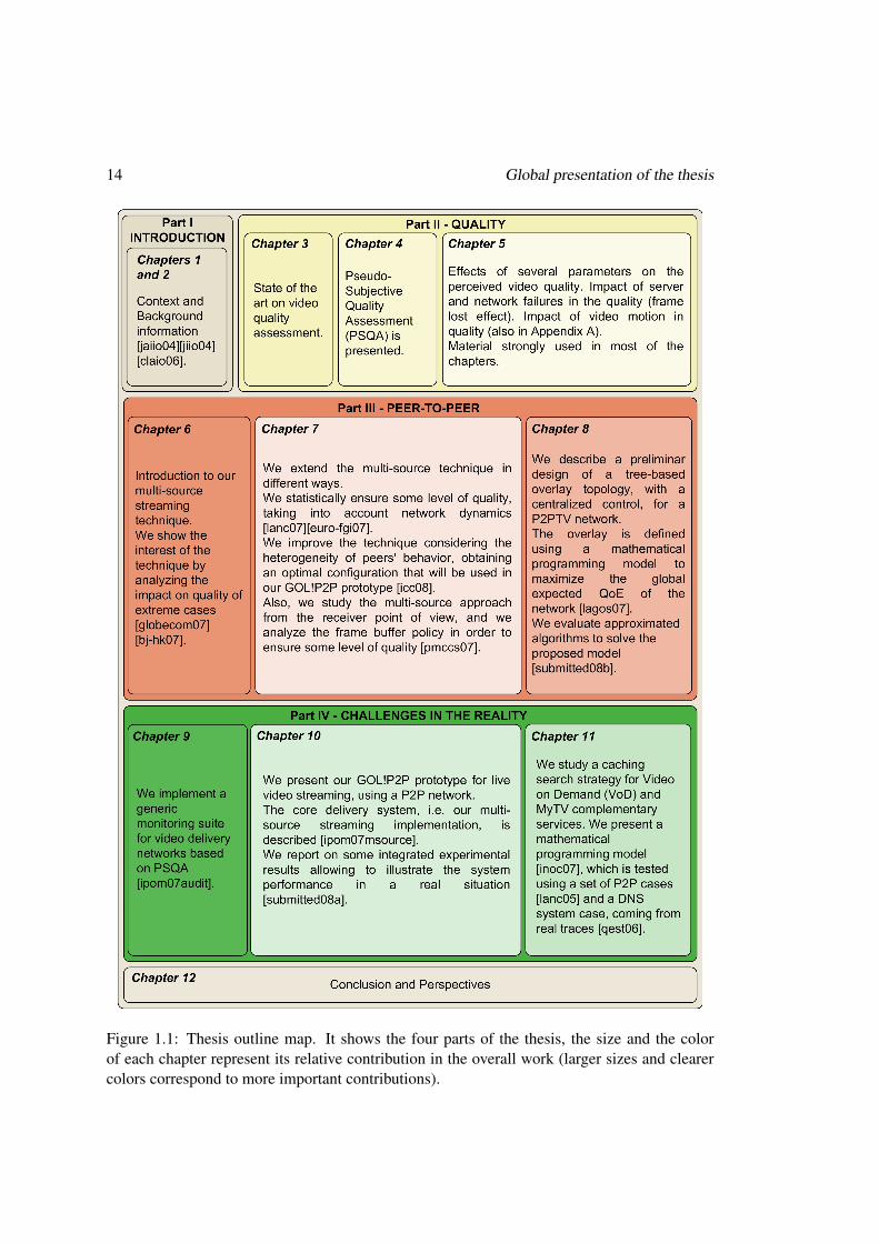
Figure 1.1: Thesis outline map. It shows the four parts of the thesis, the size and the colorof each chapter represent its relative contribution in the overall work (larger sizes and clearercolors correspond to more important contributions).

Publications 15
way the stream is decomposed on the resulting quality. Chapter 7 presents a deeper study ofour proposed multi-source streaming technique. We show, using real data, how our approachallows to compensate efficiently the possible losses of frames due to peers leaving a P2P sys-tem. We improve the technique in different ways, especially considering the peers’ dynamicsheterogeneity. We obtain an optimal multi-source streaming technique that will be used in thesequel chapters. In this chapter we also study the multi-source approach from the receiver pointof view, and we define a frame buffer policy in order to ensure some level of quality.Chapter 8 explores a preliminary design of a tree-based overlay topology, with a centralizedcontrol, for a P2PTV network. We consider the problem of selecting which peer will servewhich other one, i.e. the topology construction. A mathematical programming formulationmodels the problem, while a set of proposed approximated algorithms solves it.
Part IV CHALLENGES IN THE REALITY. Chapter 9 presents a monitoring suite fora generic video delivery network. It measures in real–time and automatically, the perceivedquality at the client side by means of the PSQA methodology.Chapter 10 presents our GOL!P2P prototype for robust delivery high quality live video. It ex-plains the core delivery system, i.e. the multi-source streaming implementation, and it presentsthe global architecture and its main components.In Chapter 11 we study the problem of content discovery for the VoD and MyTV complemen-tary services. In particular, a mathematical programming model of the caching search strategyfor these services is analyzed.
Figure 1.1 shows a outline map of the thesis, combined with the contributions of eachchapter (larger size chapters and clearer color chapters imply more important contributions).
1.4 Publications
This section contains the list of papers published as a result of this PhD thesis work.
[bj-hk07] Rodríguez-Bocca, P., Exploring Quality Issues in Multi-Source Video Streaming, in:2nd Beijing-Hong Kong International Doctoral Forum: Web, Network, and Media Computing(BJ-HK Phd Forum’07). Best Paper Award in the area of Network Multimedia Applicationsand Systems., Hong Kong, SAR, 2007.
[claio06] Rodríguez-Bocca, P. and H. Cancela, Mecanismos de descubrimiento en las Redes deContenido, in: XIII Congreso Latino-Iberoamericano de Investigación Operativa (CLAIO’06),Universidad de la República, Montevideo, Uruguay, 2006.
[euro-fgi07] Rodríguez-Bocca, P., H. Cancela and G. Rubino, Modeling Quality of Experiencein Multi-source Video Streaming, in: 4th Euro-FGI workshop on “New trends in modelling,quantitative methods and measurements” (Euro-FGI WP IA.7.1), Ghent, Belgium, 2007.

16 Global presentation of the thesis
[globecom07] Rodríguez-Bocca, P., H. Cancela and G. Rubino, Perceptual quality in P2P videostreaming policies, in: 50th IEEE Global Telecommunications Conference (GLOBECOM’07),Washington DC, United States, 2007.
[icc08] da Silva, A. P. C., P. Rodríguez-Bocca and G. Rubino, Optimal quality–of–experiencedesign for a p2p multi-source video streaming, in: IEEE International Conference on Commu-nications (ICC 2008), Beijing, China, 2008.
[inoc07] Rodríguez-Bocca, P. and H. Cancela, Modeling cache expiration dates policies in con-tent networks, in: International Network Optimization Conference (INOC’07), Spa, Belgium.,2007.
[ipom07audit] Vera, D. D., P. Rodríguez-Bocca and G. Rubino, QoE Monitoring Platform forVideo Delivery Networks, in: 7th IEEE International Workshop on IP Operations and Man-agement (IPOM’07), San José, California, United States, 2007.
[ipom07msource] Rodríguez-Bocca, P., G. Rubino and L. Stábile, Multi-Source Video Stream-ing Suite, in: 7th IEEE International Workshop on IP Operations and Management (IPOM’07),San José, California, United States, 2007.
[jaiio04] Rodríguez-Bocca, P. and H. Cancela, Redes de contenido: un panorama de sus car-acterísticas y principales aplicaciones, in: 33th Argentine Conference on Computer Scienceand Operational Research, 5th Argentine Symposium on Computing Technology (JAIIO’04),Córdoba - Argentina, 2004.
[jiio04] Rodríguez-Bocca, P. and H. Cancela, Introducción a las Redes de Contenido, in: Jor-nadas de Informática e Investigación Operativa (JIIO’04), Montevideo, Uruguay, 2004.
[lagos07] Cancela, H., F. R. Amoza, P. Rodríguez-Bocca, G. Rubino and A. Sabiguero, A ro-bust P2P streaming architecture and its application to a high quality live-video service, in: 4thLatin-American Algorithms, Graphs and Optimization Symposium (LAGOS’07), Puerto Varas,Chile, 2007.
[lanc05] Rodríguez-Bocca, P. and H. Cancela, A mathematical programming formulation ofoptimal cache expiration dates in content networks, in: Proceedings of the 3rd internationalIFIP/ACM Latin American conference on Networking (LANC’05) (2005), pp. 87–95.
[lanc07] Rodríguez-Bocca, P., H. Cancela and G. Rubino, Video Quality Assurance in Multi-Source Streaming Techniques, in: IFIP/ACM Latin America Networking Conference (LANC’07).Best paper award by ACM-SIGCOMM, San José, Costa Rica, 2007.
[pmccs07] da Silva, A. P. C., P. Rodríguez-Bocca and G. Rubino, Coupling QoE with de-pendability through models with failures, in: 8th International Workshop on PerformabilityModeling of Computer and Communication Systems (PMCCS’07), Edinburgh, Scotland, 2007.

Publications 17
[qest06] Cancela, H. and P. Rodríguez-Bocca, Optimization of cache expiration dates in contentnetworks, in: Proceedings of the 3rd international conference on the Quantitative Evaluationof Systems (QEST’06) (2006), pp. 269–278.
[submitted08a] Rodríguez-Bocca, P. and G. Rubino, A QoE-based approach for optimal designof P2P video delivering systems, submitted.
[submitted08b] Martínez, M., A. Morón, F. Robledo, P. Rodríguez-Bocca, H. Cancela andG. Rubino, A GRASP algorithm using RNN for solving dynamics in a P2P live video streamingnetwork, submitted.

18 Global presentation of the thesis

Chapter 2
Background
Some background information is needed to understand this work. This chapter briefly recallsthe main needed concepts.
2.1 Digital Video Overview.
Digital video is a video representation using digital signals. It refers to the capturing, manipu-lation, distributing and storage of video in digital formats, allowing it to be more flexible andrapidly manipulated or displayed by a computer.
Digital video enabled a revolution in the associated research areas. Video compression re-ceived an important research attention from the late 1980’s. It enabled a variety of applicationsincluding video broadcast over digital cable, satellite and terrestrial, video-conferencing, digi-tal recording on tapes and DVD’s, etc. Video communication over best-effort packet networksstarted in the mid 1990’s, with the growth of the Internet. In the Internet, the packet losses,the time-varying bandwidth, and the delay and jitter, are the main difficulties faced by videodelivery.
2.1.1 Compression and Standard Coding of digital video
Video compression is the technique designed to eliminate the similarities or redundancies thatexist in a video signal. Roughly speaking, a digital video signal is a temporal sequence of dig-ital pictures (or frames). Consecutive pictures in the sequence have temporal redundancy sincethey typically show some movement over the same objects. Inside a picture there is spatial andcolor redundancy, where the values of nearby pixels are correlated. Besides eliminating the re-dundancy, the most used compression techniques are lossy, where they encode only perceptionrelevant information, reducing the irrelevant data and increasing the compression ratio.
A compression method is completely specified by the encoder and decoder systems, jointlycalled CODEC (enCOder/DECoder). Main codecs today are based on the standards proposedby the Moving Pictures Expert Group (MPEG).
MPEG-2 is an umbrella of international compression standards [167], developed by the
19
20 Background
MPEG group. Several of its parts were developed in a joint collaborative team with ITU-T(for instance, the specific codecs H.261 [176] and H.263 [177]). After the success of MPEG-2,the MPEG-4 was standardized by the same teams. The key parts to be aware of are MPEG-4part 2 [169] (used by codecs such as Xvid [354]) and MPEG-4 part 10 [168] (known also asMPEG-4 AVC/H.264). In addition to standard codecs, there are some proprietary ones. Themain and most used examples are RealVideo [268] and Windows Media Video (in the processof standardized).
Standard codecs and proprietary codecs use the same compression principles, and thereforeby understanding one of them we can gain a basic understanding of the whole compressionarea.
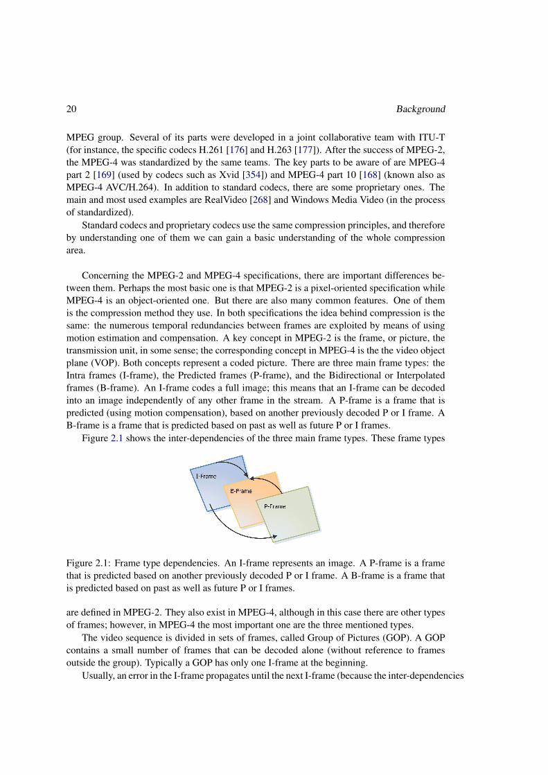
Concerning the MPEG-2 and MPEG-4 specifications, there are important differences be-tween them. Perhaps the most basic one is that MPEG-2 is a pixel-oriented specification whileMPEG-4 is an object-oriented one. But there are also many common features. One of themis the compression method they use. In both specifications the idea behind compression is thesame: the numerous temporal redundancies between frames are exploited by means of usingmotion estimation and compensation. A key concept in MPEG-2 is the frame, or picture, thetransmission unit, in some sense; the corresponding concept in MPEG-4 is the the video objectplane (VOP). Both concepts represent a coded picture. There are three main frame types: theIntra frames (I-frame), the Predicted frames (P-frame), and the Bidirectional or Interpolatedframes (B-frame). An I-frame codes a full image; this means that an I-frame can be decodedinto an image independently of any other frame in the stream. A P-frame is a frame that ispredicted (using motion compensation), based on another previously decoded P or I frame. AB-frame is a frame that is predicted based on past as well as future P or I frames.
Figure 2.1 shows the inter-dependencies of the three main frame types. These frame types
Figure 2.1: Frame type dependencies. An I-frame represents an image. A P-frame is a framethat is predicted based on another previously decoded P or I frame. A B-frame is a frame thatis predicted based on past as well as future P or I frames.
are defined in MPEG-2. They also exist in MPEG-4, although in this case there are other typesof frames; however, in MPEG-4 the most important one are the three mentioned types.
The video sequence is divided in sets of frames, called Group of Pictures (GOP). A GOPcontains a small number of frames that can be decoded alone (without reference to framesoutside the group). Typically a GOP has only one I-frame at the beginning.
Usually, an error in the I-frame propagates until the next I-frame (because the inter-dependencies

Digital Video Overview. 21
of the other frames in the GOP). Errors in the P-frames propagate until the next I-frame or P-frame. B-frames do not propagate errors. The more I-frames the video has, the more robustto failures it is. However, having more I-frames increases the video size. In order to savebandwidth, videos prepared for Internet broadcast often have only one I-frame per GOP. InMPEG-2, the GOP size is around 20 frames, while in MPEG-4, it rises to 250 frames. It is pos-sible because the MPEG-4 coding has more flexibility and expressiveness then its predecessor,allowing a better compression with greater use of P and B frames.
2.1.2 Digital video applications and Streaming Issues
The digital video can be stored, for future use, or transmitted, for a remote playback. Thereexist a diverse range of video applications, which have very different properties and constraints.
For instance, a video communication application can be for one-to-one communication(like video calls or video-on-demand), for one-to-many communication (like video conferenc-ing and multiplayer games), or for one-to-all communication (like broadcast TV). The com-munication can be interactive or bi-directional (like video conferencing), or non-interactive(like broadcast TV or video-on-demand). The video can be encoded in real–time (live TV), orpre-encoded (like video-on-demand).
The specific application constraints strongly influence the design of the system. A sum-mary of the most successful video delivery networks are presented in section 2.2. Next, webriefly present the mechanisms to deliver video over packet networks.
Video streaming stands for the simultaneous delivery and playback of video over packetnetworks [19]. Each frame must be delivered and decoded by its playback time, therefore thesequence of frames has an associated sequence of deliver/decode/playback deadlines, knownas real–time constraints.
Basically, in a streaming mechanism, the video is split into pieces (in a particular containerformat), which are sequentially transmitted over the network (with a transport protocol), andthe receiver decodes and reproduces the video as the components of the stream arrive.
Nowadays there are many different container formats such as MPEG-TS, MPEG-PS, AVI,OGM and so on. Many of these formats focus on some specific application type. For exampleMPEG-PS is suitable for transmission in a relatively error-free environment, while MPEG-TS(Transport Streams) is suitable for transmission in which there may be potential packet lossesor corruption by noise. In this thesis we used MPEG-TS as our container format.
The MPEG-TS specification basically addresses two main features, the multiplexing ofdigital video and audio and the output synchronization. It also defines rules for conditionalaccess management and multiple program transport streams (i.e., sending more than one pro-gram at a time). The audio or video encoder output is called an Elementary Stream (ES). Ina further step, elementary streams are packetized into smaller units, generating the PacketizedElementary Stream (PES). Then, these PES are packetized, in turn, into still smaller packetscalled transport stream (TS) packets. At this level is where the audio and video multiplexingis done, creating an unique stream called transport stream (TS). Finally this transport streamis encapsulated into some transport protocol packets in order to send it through the network.Nowadays there are various transport protocols suitable for the streaming transport over a net-

22 Background
work; some of them are: User Datagram Protocol (UDP), Real-time Transport Protocol (RTP)and Hypertext Transfer Protocol (HTTP)1. Each one of these protocols has its own advantagesin specific situations, together with some disadvantages when using them in certain types ofscenarios. UDP [142] is a non-connection-oriented protocol, appropriate for live streaming,for instance. RTP [146] was specifically designed to stream media over networks. It was builton the top of UDP and, as its name suggests, it is designed for real-time streaming. Finally,HTTP [148] is a connection-oriented protocol that guarantees correct delivery of each bit inthe media stream. Actually 40% of the Internet streaming is transported over HTTP [79], andin most cases proprietary streaming protocols are used. An HTTP stream has the enormousadvantage of bypassing the firewalls protections. This makes it very popular in the Internetusers community. HTTP is the protocol typically used in Internet TV systems.
2.2 Video Delivery Networks
A Video Delivery Network (VDN) is a system that delivers video transparently to end users.The area of Video Delivery Networks is growing nowadays, because of the larger bandwidthavailable on the access networks (on the Internet, cellular networks, private IP networks, etc.),the new business models proposed by video content producers, and the capability of new hard-ware to receive video streams.
Service providers have developed many types of services using video streaming, for in-stance: broadcast TV (or live TV), video on demand (VoD), video conferencing, security mon-itoring, etc. In this work we concentrate on VoD and live TV services. Also, different videoformats and resolutions are being used, depending on the nature of the service and the networkconstraints. From the network point of view, VDNs have many different architectures, andthere are specific technological challenges associated with each of them. The most success-ful networks today can be classified into the following categories: Digital Cable and Satellite,Internet Television, P2PTV, IPTV, and Mobile TV.
We describe next the main characteristics of the most important Video Delivery Network(VDN) architectures, with special focus on the main factors that affect the overall Quality ofExperience (QoE).
2.2.1 A Simple Network Model.
A generic high level end-to-end video services delivery network model is shown in Figure 2.2.The data layer of the network is composed of five stages: acquisition, encoding packetization,distribution, and decoding. There are many possibles sources for video acquisition. Someexamples are analog and digital storage (video tapes, hard disk) or live events using videorecorders. Uncompressed video has a large amount of redundancy in the signal. This redun-dancy is eliminated (or reduced) when adapting the signal to the specific transmission networkcapacity by the encoding process, a task typically done by specific hardware or generic servers.
1There are other important proprietary streaming protocols, like Microsoft Media Server (MMS), RealMedia,etc.

Video Delivery Networks 23
Figure 2.2: Video Delivery Network model architecture. Data layer of the network is composedof five stages: acquisition, encoding, packetization, distribution, and decoding.
Important parameters for the overall quality are defined in this encoding process. For exam-ple, the bit rate used and the choice between constant and variable rates (CBR or VBR), theGOP (Group of Pictures, see below) structure, the frame rate possible, rate shaping, etc. Theencoded video signal is multiplexed with an associated encoded audio flow, and it is dividedinto small pieces to simplify its distribution. This process is known as packetization (typically,MPEG packetization). Then, an adaptation to the transport layer is performed, also known aspacketization. Usually, RTP or UDP is the protocol used for the transport packetization. Packe-tizations are normally performed by the encoder or streaming server. From the head-end (centerof acquisition, encoding and packetization) to the final user’s terminal, the video flow travelsthrough several networks. First, a transport network (typically IP over MPLS or ATM) sendsthe video to the nearest provider point of presence. From there to the home, the access networkis used, typically based copper or coaxial, and this is the bandwidth capacity bottleneck of theentire system. Finally, a distribution inside the user’s house is needed. The home network usesEthernet, coaxial or wireless connections. This distribution can occasionally be supported bythe service provider. Video decoding performs stream de-multiplexing, clock synchronizationand signal decoding. Usually the video decoding process is hardware-based. The video displaydevice (typically a television set) is an important components of the final video quality; someexamples of the associated factors are the type of screen, its size, or its resolution.
Internet Television. On the Internet, the majority of VDN have a traditional CDN (ContentDelivery Network) structure [72, 346], where a set of datacenters absorbs all the load, that is,concentrates the task of distributing the content to the customers. This is, for instance, the caseof msnTV [225], YouTube [360], Jumptv [187], myTVPal [228], etc., all working with specific

24 Background
video contents2.
P2PTV. Another method becoming popular in the Internet these days consists in using theoften idle capacity of the clients to share the distribution of the video with the servers, throughthe now mature Peer to Peer (P2P) systems. Today, the most successful P2PTV networks areiMP [27] (from BBC), Joost [185], PPlive [260] and TVUnetwork [326], PPstream [261], Sop-Cast [312], TVAnts [325]. These are virtual networks developed at the application level overthe Internet infrastructure. The nodes in the network, called peers, offer their resources (band-width, processing power, storing capacity) to the other nodes, basically because they all sharecommon interests (through the considered application). As a consequence, as the number ofcustomers increases, the same happens with the global resources of the P2P network. This iswhat we call scalability in the Internet. Clearly, using a P2P infrastructure for video distribu-tion appears to be a good idea, due to the high requirements in terms of bandwidth of theseapplications, and we observe that streaming services in VoD (Video on Demand) have actuallysimilar characteristics than popular P2P systems for file sharing and distribution. However,real-time video streaming (live TV) has different and strong constraints that imply a series ofspecific technical problems because of the before-mentioned P2P dynamics.
IPTV. IPTV is a network architecture where digital broadcast television and VoD servicesare delivered using the Internet Protocol over a dedicated and closed network infrastructure.IPTV is typically supplied by a broadband operator together with VoIP and Internet access (theset of services is called “Triple Play”). IPTV is not TV that is broadcasted over the publicInternet, as in the previously mentioned Internet TV or P2PTV, it is another competitor in thismarket. Given the architecture complexity of IPTV and the typical lack of experience in videoof traditional telecommunication companies, in general the IPTV solutions are provided by anintegrator. Well known names in the market are Alcatel [9], Siemens [309], and Cisco [59].
MobileTV. MobileTV is a name used to describe a video delivery service (live and VoDvideo) to mobile phone devices. MobileTV is typically supplied by a mobile operator. Onedifference with the previous described systems is that MobileTV has two possible architec-tures at the access network: either it uses the two-way cellular access network (W-CDMA,CDMA2000, GSM, GPRS, etc.) or it relies on a dedicated digital broadcast network (DVB-H,DMB, TDtv, ISDB-T, etc.). It is expected that the cellular network will be used for unicast de-livery (i.e. VoD) and the broadcast network will be used for multicast services (live TV). Theimplementations start to comply with the IP Multimedia Subsystem (IMS) architecture [1],and, as in the IPTV case, this market is dominated today by the main integrators.
Digital Cable and Satellite. The difference between IPTV and Digital Cable concentratesat the distribution stage. Digital Cable provides television to users via radio frequency sig-nals transmitted through coaxial cables and/or optical fiber distribution networks. It may beeither a one-way or a bidirectional distribution system. In the DVB-C standard, Digital Cable
2In general, the technologies used are derived from those associated with Web applications, thus based on theHypertext Transfer Protocol (HTTP) [184, 203, 311].

Video Delivery Networks 25
uses a spectrum with more than 100 carriers of 6 MHz channels, typically used to carry 7-12standard digital channels (MPEG-2 MP@ML3 streams of 3-5 Mbps). The modulation is theQuadrature amplitude modulation (QAM) technology, in the 64-QAM and 256-QAM versions.The abbreviation CATV originally meant “Community Antenna Television”; however, CATVis now usually understood to mean “Cable TV”. The Digital Satellite television uses a satelliteto distribute the signal to the users. It typically uses the Quadrature Phase-shift keying (QPSK)digital modulation, and the standards MPEG-2 or MPEG-4 AVC, and DVB-S (or DVB-S2).
2.2.2 Quality-of-Experience (QoE) in a VDN.
A common challenge of any Video Delivery Network deployment is the necessity of ensuringthat the service provides the minimum quality expected by the users. Quality of Experience(QoE) is the overall performance of a system from the users’ perspective 4. QoE is basicallya subjective measure of end-to-end performance at the service level, from the point of view ofthe users. As such, it is also an indicator of how well the system meets its targets. To identifyfactors playing an important role on QoE, some specific quantitative aspects must be consid-ered [87]. For video delivery services, the most important one is the perceptual video qualitymeasure.
In the previous subsection, we described the most successful classes of VDN nowadays.Depending on the service provided, each type of VDN has its own specific protocols and com-ponents. First, observe that there are no significant differences on the video sources of thenetwork. Obviously, the quality of the original video (analog or digital) greatly affects theencoding efficiency and the overall QoE. Certainly, better quality is expected in dedicatednetworks as in the IPTV, Digital Cable and Satellite cases (for example, these networks typ-ically use MPEG-2 or MPEG-4 video sources, in comparison with P2PTV that uses hometechnology). Video encoding is accomplished using video codecs appropriate to the particularnetwork. In the Internet environment (Internet TV and P2PTV), the video encoders are imple-mented with dedicated servers, or simply with home PCs. In the dedicated networks (IPTV,MobileTV, cable...) a hardware appliance encoder is preferred.
The encoder parameters (like the encoder standard used, the bit rate, the GOP structure,CBR/VBR, etc.) are defined taking into account the transmission method and the bandwidthrequirements. Since encoders and decoders are basically software-based, there is a large free-dom for the specific designs, in the Internet world. The standard case for the applications isthe use of proprietary codecs (sometimes MPEG-4 – xvid, H.264, sometimes SMPTE VC-1 –Windows Media 9).
3The MPEG-2 specification defines profiles and levels to allow specific applications to support only a subset ofthe standard. While the profile defines features (such as the compression algorithm), the level defines the quantita-tive capabilities (such as maximum bit rate) in this profile. At least the main profile (MP) and the main level (ML)(for instance the DVD quality) are accepted in the digital cable and satellite.
4Sometimes QoE is confused with QoS (Quality of Service). QoS is related to objective measures of perfor-mance at the network level and from the network point of view. QoS also refers to the protocols and architecturesthat enable to provide differentiated service levels, as well as managing the effects of congestion on applicationperformance.

26 Background
In IPTV and digital cable and satellite, MPEG-2 implementations are being smoothly re-placed by new encoders such as H.264 and VC-1. In MobileTV, following the 3GPP recom-mendations, MPEG-4 Part 2 is used. The bit rate affects the quality substantially. Internet TVand P2PTV typically use broadband home connections (of about 500 Kbps). In MobileTV, theaccess network limits the bandwidth available to about 100 Kbps in 2G networks and at most2 Mbps in the case of 3G networks. In IPTV and digital Cable and Satellite a minimum of 12to 24 Mbps is recommended.
The MPEG packetization used to multiplex video and audio, and to divide it into smallpieces in order to simplify the distribution. Usually MPEG-TS is used for this task, for singlechannel distribution (Single Program Transport Streams) as in IPTV, or for multiple chan-nel distribution (Multiple Program Transport Stream) as in Digital Cable. In Internet TV andP2PTV an important amount of standards and proprietary protocols are used. After the packeti-zation phase, the transport packetization is performed, typically by the encoder or by streamingserver. Again, there are many standards and proprietary protocols for this processes in the In-ternet.
The distribution characterizes the different VDN architectures considered. The distributionintroduces some delay, jitter, and loss in the stream. In live TV and VoD the most importantfactor is the packet loss because the video quality and the overall QoE degrades severely withit (in Chapter 5 we study the effects of several factors on the perceived video quality, andthe most important ones are referred to the distribution). Fixed access of IPTV and digitalcable (e.g., ADSL2+, cable modems, Ethernet, etc.) can control the QoS of the distributionwith intelligent priority-marking algorithms, except in the home network where wireless isused (Wi-Fi), degradating potentially the quality. Digital Satellite television and mobileTVdepend significantly on the variable environment conditions. In P2PTV the access networkis an overlay network of peers that give (part of) their bandwidth to the others. The mainproblem here is that peers connect and disconnect with high frequency, in an autonomous andcompletely asynchronous way. This means that the main challenge in P2P design is to offerthe quality needed by the clients in such a highly varying environment, trying to minimizepackages losses. A set of methods are being used in access networks to mitigate packet losses.Some examples are Forward Error Correction (FEC), retransmission, selective discard, and inparticular situations as in P2PTV, the multiple source or the multiple path streaming.
Video decoding is done by a dedicated hardware (Set-Top-Box for IPTV, Cable, Satelliteand mobileTV), except in the Internet where a personal computer is typically used. Finally, asstated above, the television terminal is another important component of the QoE, with, as mainassociated factors, the type of screen, its size, or its resolution.
The components of a video delivery network are summarized in Figure 2.3 and its protocolsare shown in Figure 2.4.
2.2.3 Summary
A Video Delivery Network (VDN) is a system that delivers video transparently to end users.VDNs have different architectures: Digital Cable and Satellite, Internet Television, P2PTV,IPTV, and Mobile TV. No matter how well-designed a network is or how rigorous its QoScontrols are, there is always the possibility of failures in its components, of congestion, or of

Video Delivery Networks 27
Figure 2.3: Components of a Video Delivery Network.
Figure 2.4: Protocols of Global architecture.

28 Background
errors creeping into the video stream. Therefore, it is necessary to monitor and to measure theoverall quality in a Video Delivery Network, and especially the perceived quality, representingthe user’s point of view. In next section we study with more detail the Video Delivery Networkused in the Internet (Internet TV and P2PTV). In Chapter 9 we detail a general video deliverynetwork monitoring suite (applicable to all the VDN architectures), that measures, in real–time and automatically, the perceived quality at the client side. In Chapter 10 we present ourGOL!P2P prototype, a P2P architecture for real–time (live) video distribution.
2.3 Peer-to-Peer Network Architecture for Video Delivery on In-ternet
For the specific context of the Internet, the presented VDN architectures (Internet TV andP2PTV) are enclosed inside the general concept of Content Networks. After introducing themin general, we present, in the particular case of video flows, the Content Delivery Networks(CDN) and the Peer-to-Peer networks (P2P). Finally, we focus on the state of the art of thePeer-to-Peer network design for video delivery.
2.3.1 Introduction, the Content Networks
A Content Network is a network where the addressing and the routing of the information isbased on the content description, instead of on its physical or logical location [199, 200, 216].Content networks are usually virtual networks built over the IP infrastructure of Internet or ofa corporative network, and use mechanisms to allow accessing a content when there is no fixedsingle link between the content and the host (or hosts) where this content is located. Even more,the content is usually subject to re-allocations, replications, and even deletions from the differ-ent nodes of the network. In the last years many different kinds of content networks have beendeveloped and deployed in widely varying contexts, they include (see Figure 2.5): the domainname system [39, 143, 144, 242], peer-to-peer networks [30, 60, 82, 88, 89, 115, 190, 230,305], content delivery networks [7, 58, 247–250], collaborative networks [33, 34, 121, 240],cooperative Web caching [94, 98, 181, 262, 269, 313], subscribe-publish networks [23, 45],content-based sensor networks [92, 129, 130], backup networks [85, 198, 287, 288], distributedcomputing [69, 96, 112, 305], instant messaging [141, 180], multiplayer games [84], and searchengines [116, 356].
The ability of Content Networks to take into account different application requirements(like redundancy and latency) and to gracefully scale with the number of users have been amain factor in this growth [251, 262, 272]. Other motivations for their deployment are thepossibility to share resources (for example in P2P networks), and the simple design to avoidcentralized, single failure points or bottlenecks.
In [274, 276, 277, 279] we present a taxonomy of Content Networks, based on their ar-chitectures. Some of the characteristics studied were the decentralization of the network, thecontent aggregation and the content placement. We also analyze their behavior, in terms ofperformance and scalability.

Peer-to-Peer Network Architecture for Video Delivery on Internet 29
Figure 2.5: Example of current Content Networks (CNs).
Depending on the specific application of the content network, and mainly on the contentdynamics in the network, different architecture designs are used. The design areas of a contentnetwork are:
• Content Discovery. The objective of a content network is to transparently present thecontents to the end users, i.e. present a consistent global view of the contents. In orderto reach this objective, the network must be able to answer each content query with themost complete possible set of nodes where this content can be found; this correspondsto discovering the content location in the most effective and efficient possible way.
The content discovery is introduced in Section 2.4, and studied in depth in Chapters 8and 11. In the P2P Section 2.3.3, we reference it in our particular context.
• Content Distribution. Knowing the nodes where each specific content is to be found, aclient of the network retrieves the content of these sources.
The task of delivering the content is call content distribution. Depending on the kindof content, different restrictions must be considered. Some unique contents (like chatsor multiplayer games) have to be exclusively distributed from the source, file sharing istypically distributed from all the replicated sources in a best effort form, video streaminghas real–time restrictions, etc.
The content distribution has been intensively studied in each kind of content network, inorder to improve the efficiency of the distribution, or the availability of the content. It isalso studied in te context of P2P networks as a mechanism with incentives to share, andto avoid or mitigate the free-riders (peers that only consume the content but not servethem to other ones).

30 Background
In our work we focus on the video distribution in order to improve the quality-of-experience (QoE). See 2.3.3.3 for the special P2P case. Our multi-source streamingtechnique is presented in chapters 6 and 7.
• Network Dynamics. The network effect is defined as the phenomenon whereby a prod-uct or service becomes more valuable as more customers use it, thus encouraging evenincreasing numbers of customers [235, 236]. Usually, content networks have a veryhigh network effect potential, specially P2P networks, and it is considered in depth, forexample with game theory.
If two networks offer the same kind of content, they are in competition. Also the networkdynamics is studied in the competence context.
• Others. Other design factors are commonly studied, like security, anonymity, interoper-ability, etc.
These last years have seen an explosion on the design and deployment of different kindsof content networks, in most cases without a clear understanding of the interaction betweennetwork components neither of the tuning of the network architecture and parameters to ensurerobustness and scalability and to improve performance. This in turn has led to a still small(but growing) number of empirical studies (based on large number of observations of a givennetwork activity) [186, 272, 300, 302, 361], and of analytical models which can be fitted to theobservations in order to better understand and possibly to predict different aspects of networkbehavior [99, 251, 262, 358, 359].
2.3.2 Content Networks for Video Delivery on Internet
In Section 2.2 we introduce two main architectures for the Internet-based Video Delivery Net-works: Internet TV and P2PTV. In the present section we will explain them in depth. Depend-ing on their number of simultaneous clients, Internet TV is deployed using a simple ServerFarm or a scalable Content Delivery Network (CDN). On the other hand, P2PTV is based onPeer-to-Peer (P2P) systems.
Different architectures are needed for the same service because of scale and cost reasons(the deployment of this service on Internet is very expensive, mainly due to the bandwidthcosts).
2.3.2.1 Scale and Cost Problem of Live-video Delivery on Internet
Following [12], the scale and cost problem results from the fact that only one-to-one commu-nications are available on Internet, which implies sending a different copy of the video to eachclient.
The bandwidth is the most expensive resource on Internet, and video delivery is one of theservices that most demand it. In particular, the cost of live video delivery is proportional tothe number of simultaneous clients, and nowadays it is the first limitation for the expansion ofavailability and of diversity of video content on Internet. Moreover, live-video delivery is hardto scale without a strict planning because the streaming of popular videos cause high congestion
Peer-to-Peer Network Architecture for Video Delivery on Internet 31
in most Internet sectors. Congestion implies high number of losses in the distribution, andtherefore a significant perceived quality degradation by clients.
But point-to-point communication is not a limitation of the Internet Protocol (IP) standard,it is a traditional Internet Service Provider (ISP) business rule based on lack of standards ma-turity and revenue preservation5. In IP, one-to-one communication is called unicast, and thestandard also allows one-to-all communication (broadcast), and one-to-many communication(multicast). While in IP broadcast, data is sent (only once by the source) to all possible destina-tions, in IP multicast, data is sent (only once by the source) to all requesters that have registeredtheir interest in it from that source. IP broadcast and IP multicast are limited to dedicated net-works (corporate or enterprise networks). Applications that use IP multicast include IPTVarchitectures (see Section 2.2), videoconferencing, distance learning, corporate communica-tions, software distribution, routing protocols, stock quotes, news, etc. IP Multicast [153, 154]is able to minimize the bandwidth consumption in the network. A requester must join a multi-cast group (by using the Internet Group Management Protocol (IGMP) [156, 162]) to receive aparticular multicast content. Routers build distribution trees for each multicast group (by usingProtocol Independent Multicast (PIM) [158, 159, 161]) which replicate and distribute multicastcontent to all requesters that are in this group.
2.3.2.2 Content Delivery Networks (CDN): global scalability
Without IP multicasting on Internet, video delivery infrastructure usually begins with a serverfarm, using unicast communication. The farm allows high availability and load balancing be-tween its servers. It has an available (and expensive) bandwidth, B Kbps, that is shared bythe set of servers (usually uniformly). If the stream consumes bw Kbps, the total number ofsimultaneous clients has to be less than B/bw. It is possible to increase the number of clients,growing the available bandwidth B (increasing the costs) or reducing the video quality (reduc-ing bw). For example if bw = 500 Kbps, and we have four thousands clients (a small numberfor a global system), we need more than B = 2 Gbps (that is a very high value for most busi-ness models). Actual servers can stream at approximately 800 Mbps, and can be consideredas extremely dependable. Nevertheless, when the number of clients increases, the server farmneeds to be upgraded to several server farms, or to a Content Delivery Network to avoid bot-tlenecks at the farm, and to reduce latency to end users.
Current successful Internet-based Video Delivery Networks have a traditional Content De-livery Network (CDN) structure. A Content Delivery Network (CDN) [140, 264, 332] is asystem of servers located at strategic points around the Internet that cooperate transparently todeliver content to end users. Basically, all nodes in a CDN can serve the same content. Thepreference for a particular node to serve a particular client, is decided using (possible propri-etary) protocols between servers to identify which is the best one to do the task. Each particular
5There are some exceptions to this rule. MBONE [91] (short for “Multicast Backbone”) was a virtual IP networkcreated to multicast video from the Internet Engineering Task Force (IETF) meetings. MBONE was used by severaluniversities and research institutions. Recently, the U.S. Abilene Network [3] has been created by the Internet2community and natively support IP multicast. The BBC multicast initiative [28] is another example of currentefforts.

32 Background
CDN has its own rules to determine the best server, usually based on network proximity, net-work congestion, etc.
The CDN approach was originally developed to improve the World Wide Web service. Itreduces client latency and network traffic by redirecting client requests to a node closest tothat client. In addition, it improves the availability of the service, avoiding single points offailures and distributed denial of service. Today, there is a wide range of academic knowl-edge that discusses different aspects of the use of CDN to WWW replication (for instance,see the books [140, 264, 332] and the surveys [184, 203, 311]). Some of the most importantaspects that differentiate each CDN approach are: the request routing mechanism that deter-mine which node will serve each client, where to replicate the content (i.e. where to placea node of the CDN in Internet, and in which node to replicate each content depending on itspopularity), how to maintain the consistency between the servers considering content changes,and how the CDN adapts to the content, server and client dynamics. Current successful CDNsare the following: Akamai, with tens of thousands of replica servers placed all over the In-ternet [7, 81]; CDNetworks, with a big deployment in Asia [50]; Globule, an open-sourcecollaborative CDN [14, 256–258]; CoDeeN [97], an academic testbed built on top of Planet-Lab [259]; etc. [247–250].
Considering that video delivery is one of the most bandwidth-demanding applications run-ning on the Internet, it is natural to think that CDNs will extend their service to video delivery aswell. Nowadays, all the commercial CDNs deployments include streaming, specially for videoon demand, because technically it is very similar to file downloading. Also particular CDNsare developed for media delivery service, for audio streaming [166, 202, 227, 265, 317, 339],and video streaming [49, 306, 335]. The most successful Internet TV deployments use a CDNarchitecture; this is, for instance, the case of YouTube [360], msnTV [225], Jumptv [187], etc.Behind the commercial CDNs, there are some academic studies [72, 193, 346].
From the scale and cost point of view, the CDN architecture solves the scalability problemof the server farm (avoiding bottlenecks); but the cost problem persists, because in a CDNa set of servers absorbs all the load (i.e. concentrates the task of distributing the content tothe customers). Therefore, as in the server farm solution, the cost is proportional to the totalnumber of simultaneous clients. In addition the cost of operating and maintaining the servers,placed worldwide, has to be considered. This operational cost usually limits CDN applicationto large commercial sites only [187, 225, 360].
Moreover, a CDN solves the scalability problem partially, for the following reasons:
• The available bandwidth is not dynamic; therefore, a CDN does not scale well with verypopular content that has flash crowd behavior [314].
• The CDN avoids bottlenecks if the CDN servers are close to the clients. For example,this is easy for a worldwide content, but impossible if some content is very popularinside a network. For example, football (soccer) matches are one of the most popularlive contents in the world, but, for instance, the “Uruguay-Brasil” match will have lot offans inside Uruguay, and it would not help much (to these fans) to have many serverslocated outside Uruguay, because they will share the same congested link to the clients.

Peer-to-Peer Network Architecture for Video Delivery on Internet 33
2.3.2.3 Peer-to-Peer Networks (P2P): cutting off the costs
From the scalability point of view, if we want to deliver video of different popularities, it seemsto be necessary to have the server as close as possible of the final client. From the cost point ofview, it would be ideal to distribute the load of the video delivery with the interested ones (theclients).
A method becoming popular these days consists of using the often idle capacity of theclients to share the distribution of the video with the servers, through the present mature Peer toPeer (P2P) systems. P2PTV are virtual networks developed at the application level, where thenodes in the network, called peers, offer their resources (bandwidth, processing power, storingcapacity) to the other nodes, basically because they all share common interests (through theconsidered application). As a consequence, as the number of customers increases, the samehappens with the global resources of the network. Moreover, the peers that serve another peercan be chosen with a proximity network criterion, avoiding bottlenecks, even more efficientlythan with CDN servers. To base the scalability on the network effect property seems a goodidea due to the high costs in terms of bandwidth of video distribution [320]. On the negativeside, the main drawback is that peers connect and disconnect with high frequencies, in an au-tonomous and completely asynchronous way. When a node leaves the network (we will refer tothis situation as a failure), it causes the loss of the information it was sending to someone else.The resources of the network as a whole are then highly dynamic, and this leads to a seriousconstraint at the control level, because the network must be robust face to these fluctuations.This is the main challenge in P2P design: to offer the quality needed by the clients in a highlyvarying environment.
Some commercial P2PTV networks for video distribution are available. The most success-ful are BBC: iMP [27] based on the VeriSign Kontiki software [192], Joost [185], PPlive [260],PPstream [261], SopCast [312], TVAnts [325], and TVUnetwork [326].
Besides the commercial networks some academic studies are SpreadIt [80], CoopNet [246]and SplitStream [48].
The challenges on a P2P network design are different according to the type of video servicedeployed. Video on Demand (VoD), for instance, has similar characteristics as popular P2Psystems for file sharing and distribution. However, real–time video streaming (live TV) hasdifferent and strong constraints that imply a series of specific technical problems difficult tosatisfy in a very dynamic environment. In the next subsection we provide a short introductionto P2P technology and discuss current approaches to live TV service.
2.3.3 Peer-to-Peer (P2P) Networks
Peer-to-Peer networking are the class of systems and applications that use distributed resourcesto accomplish some critical function in a decentralized form. The resources can be: processing,storage (particular content) and / or transmission (bandwidth). The critical functions are: dis-tributed computation, shared information, collaboration between peers, or any type of services

34 Background
that can be offered by a system with these characteristics.A series of definitions co-exist with regard to P2P networks (see [216] for a discussion).
For the rest of this document we follow the definition given by Clay Shirky [308]: a Peer-to-Peer (P2P) Network is a Content Network that takes advantage of the free resources availablein the Internet edges (i.e. the final users).
P2P networks are a particular case of Content Networks, the difference appears in somecharacteristics of the architecture and of the nodes of the network:
• First, P2P networks are composed by peers with a high level of autonomy. In particular,nodes should have the possibility of connecting and disconnecting to the network at anytime in a very flexible way. In addition, in general every node determines the quantity ofresources that it wants to share.
• Considering that the nodes can enter freely to the system to share their resources, anincentive is necessary for this participation. This incentive is in general achieved becausein a P2P network, the peers share a common aim or a common need. Therefore, there isan implicit desire to share resources naturally arising in this type of systems.
• Another consequence of the autonomy is the anonymity. Often, the sources and thereceivers of a content do not want to be known (for example for legal reasons when thecontent can be subject to copyright), or in other cases simply because this knowledge iscompletely unnecessary.
The first classification of the P2P networks that appears in the literature is on the basis ofthe type of application of the network [215, 216]:
• content sharing: file delivery, multimedia distribution, distributed storage, caching, in-formation management (discover, aggregate, filter, mining, organize, etc.), etc;
• collaboration: communication (chat, instant messaging), co-review/edit/author/create,gaming, social networks, etc;
• distributed computing: Internet/Intranet distributed computing, etc. Its applicabilityincludes the extraterrestrial life search, the genome project, market analysis, financialrisk analysis, demographic analysis, etc.
An excellent survey about this classification of Peer-to-Peer systems is [216].A classification based on the application is not sufficient to understand the different types
of designs, architectures and algorithms that coexist in the P2P world. In our previous work[274] we present a taxonomy of Peer-to-Peer networks, based on their architectures. Similarworks are [15, 32, 209]. Next, we resume our taxonomy based on two main characteristics,self-organization and decentralization.
2.3.3.1 Overlay Network: the control and routing layer
In a P2P network there are two types of exchanged data: the content itself (i.e. files, videos,etc.) and the control and routing messages (i.e. peer’ connections/disconnections, content

Peer-to-Peer Network Architecture for Video Delivery on Internet 35
publications, searches, etc.). Each P2P network has its own method to exchange each typeof data. As in Content Networks, the design problem behind the content exchange is calledcontent distribution, and the design problem behind the control messages exchange is calledcontent discovery.
With respect to the content discovery, a P2P network has to transparently present the con-tents to the end users, i.e. to present a consistent global view of the contents. In order toreach this objective, some control and routing messages have to be exchanged between peersto discover the content location in the most effective and efficient possible way.
With the control information exchanged a knowledge network is constructed. The knowl-edge is the information about the location where (in each peer) specific content is to be found.The knowledge network is usually called overlay network, and is defined as follows. The Over-lay Network is a directed graph. The nodes are the peers. If a participating peer knows thelocation of another peer, then there is a directed arc from the former node to the latter.
Self-organization. There is a common P2P classification based on how the overlay is con-structed [47, 211]. The self-organization of a P2P network can be structured or unstructured.
• Unstructured. The nodes of an unstructured overlay topology are organized arbitrarily(non deterministically), using flood (broadcast or random walks) for the content discov-ery. The content searches are propagated among the peers following the overlay topol-ogy. The participating nodes are maintained together using keep-alive messages. Usuallythese networks do not scale well because of the high amount of signalling traffic. On theother hand, they present a very high level of anonymity. The most known example ofthese networks is Gnutella [115].
• Structured. A structured organization network uses a globally consistent protocol toroute a search of other node or content. In general, they consist in some variant of a Dis-tributed Hash Table (DHT) technology. These networks construct a structured overlaywhere each node maintains a specific set of contents (or a set of content location indexes).Therefore the content searches are deterministic and efficient. In structured overlay net-works, the changes of available peers and available contents are published, a differencewith respect to unstructured overlay network where peers must look for changes. Ingeneral the protocols of these networks ensure to discover a specific content crossingat most a quantity of nodes logarithmic in the size of the network. In very dynamicsnetworks it is possible that it is not efficient enough when maintaining the informationabout changes, compared to unstructured approaches. Examples are Kademlia [214],CAN [266], Chord [316], Pastry [286, 289] and Tapestry [364].
Decentralization. There are three possible roles of a peer in a P2P network. The nodes thathave contents are source nodes, the nodes that demand these contents are requester nodes, andthe nodes that exchange control messages to present a global view of content locations in thenetwork are router nodes. A single computer may be source, requester, and router node, at thesame time.
In Content Networks, the decentralization is determined by the capacity of the network towork with several nodes of the same type (sources, requesters and routers). Considering the
36 Background
peers’ desire to share in P2P networks, always there are always many sources in these networks,limiting the concept of decentralization to the requesters and (principally) to the routers.
From the decentralization point of view, P2P networks are classified in the followingtypes [359]:
• Pure. It expresses faithfully the philosophy of a P2P network, where all the nodes playequal roles (source, requester and router) and have the same responsibilities. It is acompletely distributed network, which implies that the network can work with an arbi-trary quantity of nodes of each class, for example the requesters can ask for a contentto any node, and this node has to know how to route to some source. Examples areGnutella [115] and Freenet [60, 322].
• Hybrid. The centralized model receives the name of hybrid, because it is not a pure P2Psystem. In this case there is a central node (or a server farm) that routes all the controlmessages in the network. The requesters ask for a content to the central server, whoinforms the sources of this content. The sources distribute the content in a P2P basisto the requesters. An hybrid network can have one requester or many requesters. Forexample Napster [43, 230] has a unique router node, many sources and many requesters,whereas Seti@home [305, 347] has a unique router node, many sources of processingresources, and only one requester of this processing power.
• Hierarchical. Between the pure model and the hybrid model, the hierarchical model hasseveral router nodes. In file sharing applications, hierarchical networks are called super-peer networks. In these networks there are source/requester/router nodes called super-peers and exclusively clients nodes (source/requester) called peers. The super-peers forma backbone network of control messages, and present a global view of the content in thenetwork to themselves and to the peers (with less resources than super-peers).
This model has the potential of combining the efficiency of the content searches of thecentralized hybrid systems with the autonomy, load balancing and lack of an uniquepoint of failure of the completely distributed pure systems [358, 359]. The most knownexample of this type of networks is KaZaA [190].
Usually pure networks do not scale well, because of the peers’ heterogeneity in connectiontime and shared resources [186, 272, 300, 302, 361]. By definition there are no structuredhybrid networks. When the unstructured networks grew in quantity of nodes, arose the need ofa model who was contemplating better the peers’ heterogeneity (in connection time and sharedresources), i.e. the hierarchical model. Today, the hierarchical approach is quite frequent.
Table 2.1 resumes our taxonomy of P2P architectures (with respect to two main charac-teristics: the self-organization, and the decentralization) with several P2P networks examples.Observe that, as far as we know, there are no structured hierarchical architectures (we supposebecause of its recent deployment).
2.3.3.2 Structured Overlays for Live Video Streaming
The most popular P2P systems are those designed for file sharing. Important names areKaZaA [190], Bittorrent [30], or eMule [89], all using almost no dedicated infrastructure. The
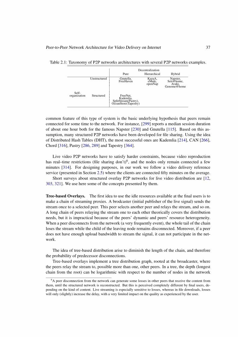
Peer-to-Peer Network Architecture for Video Delivery on Internet 37
Table 2.1: Taxonomy of P2P networks architectures with several P2P networks examples.
DecentralizationPure Hierarchical Hybrid
Unstructured Gnutella, KazaA, Napster,FreeHaven eMule, Seti@home,
openNap Avaki,Genome@home
Self-organization Structured FreeNet,
Kademlia,SplitStream(Pastry),
OceanStore(Tapestry)
common feature of this type of system is the basic underlying hypothesis that peers remainconnected for some time to the network. For instance, [299] reports a median session durationof about one hour both for the famous Napster [230] and Gnutella [115]. Based on this as-sumption, many structured P2P networks have been developed for file sharing. Using the ideaof Distributed Hash Tables (DHT), the most successful ones are Kademlia [214], CAN [266],Chord [316], Pastry [286, 289] and Tapestry [364].
Live video P2P networks have to satisfy harder constraints, because video reproductionhas real–time restrictions (file sharing don’t)6, and the nodes only remain connected a fewminutes [314]. For designing purposes, in our work we follow a video delivery referenceservice (presented in Section 2.5) where the clients are connected fifty minutes on the average.
Short surveys about structured overlay P2P networks for live video distribution are [12,303, 321]. We use here some of the concepts presented by them.
Tree-based Overlays. The first idea to use the idle resources available at the final users is tomake a chain of streaming proxies. A brodcaster (initial publisher of the live signal) sends thestream once to a selected peer. This peer selects another peer and relays the stream, and so on.A long chain of peers relaying the stream one to each other theorically covers the distributionneeds, but it is impractical because of the peers’ dynamic and peers’ resource heterogeneity.When a peer disconnects from the network (a very frequently event), the whole tail of the chainloses the stream while the child of the leaving node remains disconnected. Moreover, if a peerdoes not have enough upload bandwidth to stream the signal, it can not participate in the net-work.
The idea of tree-based distribution arise to diminish the length of the chain, and thereforethe probability of predecessor disconnections.
Tree-based overlays implement a tree distribution graph, rooted at the broadcaster, wherethe peers relay the stream to, possible more than one, other peers. In a tree, the depth (longestchain from the root) can be logarithmic with respect to the number of nodes in the network
6A peer disconnection from the network can generate some losses in other peers that receive the content fromthem, until the structured network is reconstructed. But this is perceived completely different by final users, de-pending on the kind of content. Live streaming is especially sensitive to losses, whereas in file downloads, losseswill only (slightly) increase the delay, with a very limited impact on the quality as experienced by the user.
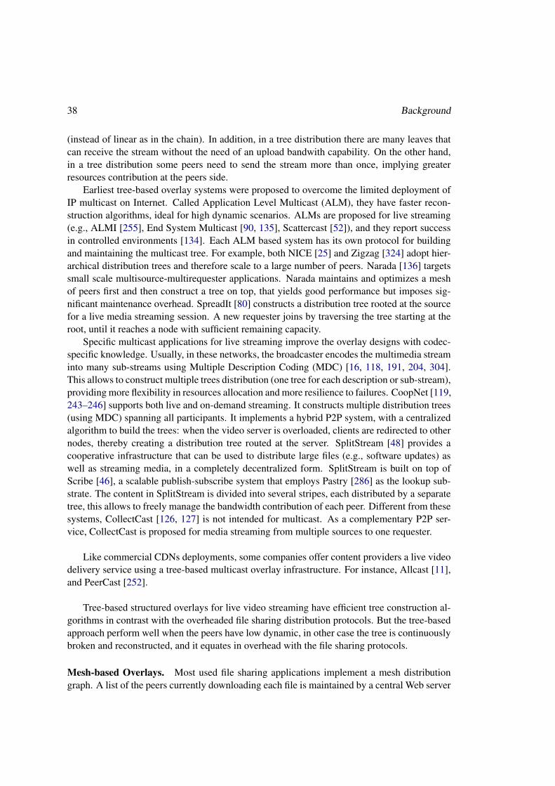
38 Background
(instead of linear as in the chain). In addition, in a tree distribution there are many leaves thatcan receive the stream without the need of an upload bandwith capability. On the other hand,in a tree distribution some peers need to send the stream more than once, implying greaterresources contribution at the peers side.
Earliest tree-based overlay systems were proposed to overcome the limited deployment ofIP multicast on Internet. Called Application Level Multicast (ALM), they have faster recon-struction algorithms, ideal for high dynamic scenarios. ALMs are proposed for live streaming(e.g., ALMI [255], End System Multicast [90, 135], Scattercast [52]), and they report successin controlled environments [134]. Each ALM based system has its own protocol for buildingand maintaining the multicast tree. For example, both NICE [25] and Zigzag [324] adopt hier-archical distribution trees and therefore scale to a large number of peers. Narada [136] targetssmall scale multisource-multirequester applications. Narada maintains and optimizes a meshof peers first and then construct a tree on top, that yields good performance but imposes sig-nificant maintenance overhead. SpreadIt [80] constructs a distribution tree rooted at the sourcefor a live media streaming session. A new requester joins by traversing the tree starting at theroot, until it reaches a node with sufficient remaining capacity.
Specific multicast applications for live streaming improve the overlay designs with codec-specific knowledge. Usually, in these networks, the broadcaster encodes the multimedia streaminto many sub-streams using Multiple Description Coding (MDC) [16, 118, 191, 204, 304].This allows to construct multiple trees distribution (one tree for each description or sub-stream),providing more flexibility in resources allocation and more resilience to failures. CoopNet [119,243–246] supports both live and on-demand streaming. It constructs multiple distribution trees(using MDC) spanning all participants. It implements a hybrid P2P system, with a centralizedalgorithm to build the trees: when the video server is overloaded, clients are redirected to othernodes, thereby creating a distribution tree routed at the server. SplitStream [48] provides acooperative infrastructure that can be used to distribute large files (e.g., software updates) aswell as streaming media, in a completely decentralized form. SplitStream is built on top ofScribe [46], a scalable publish-subscribe system that employs Pastry [286] as the lookup sub-strate. The content in SplitStream is divided into several stripes, each distributed by a separatetree, this allows to freely manage the bandwidth contribution of each peer. Different from thesesystems, CollectCast [126, 127] is not intended for multicast. As a complementary P2P ser-vice, CollectCast is proposed for media streaming from multiple sources to one requester.
Like commercial CDNs deployments, some companies offer content providers a live videodelivery service using a tree-based multicast overlay infrastructure. For instance, Allcast [11],and PeerCast [252].
Tree-based structured overlays for live video streaming have efficient tree construction al-gorithms in contrast with the overheaded file sharing distribution protocols. But the tree-basedapproach perform well when the peers have low dynamic, in other case the tree is continuouslybroken and reconstructed, and it equates in overhead with the file sharing protocols.
Mesh-based Overlays. Most used file sharing applications implement a mesh distributiongraph. A list of the peers currently downloading each file is maintained by a central Web server

Peer-to-Peer Network Architecture for Video Delivery on Internet 39
(called the tracker) in Bittorrent [30], or by a distributed number of servers (usually by the Lug-dunum software [210]) in eMule [89], or by peers with high availability (called super-peers)in KaZaA [190]. Using this list, each peer knows, at any time, a subset of other peers thatare downloading the same file (called the peer swarm). The file is distributed in pieces (calledchunks). Every peer knows which chunks are owned by the peers in its swarm, and explicitlypulls the chunks that it requires. In Bittorrent, peers request the chunks which fewest number ofpeers have (rarest-first download policy), and peers upload chunks first to the peer requestersthat are uploading data to them at the fastest rate (tit-for-tat upload policy). Other networkshave similar incentive policies to avoid free-rider peers.
Mesh-based overlays are starting to be used for live video distribution. File sharing ap-plications cannot be used directly for live video distribution, because the first chunks of thefile are not downloaded first, and therefore the file cannot be played until the download hasbeen completed. But not only the rarest-first download policy has to be changed for use in livestreaming: pull mechanisms involve overhead, that implies large buffers at the client side (toincrease the probability of finding a chunk), and therefore very high delays.
On the positive side, mesh-based overlays offer good resilience to peer failures, and theyout-perform conventional tree-based overlays because every peer is a source (no matter its up-load bandwidth capabilities). In essence, without considering protocols details, mesh-baseddistribution can be seen as a distributed tree-based mechanism for each chunk.
Besides a few academic studies [78, 321, 336, 351, 352], some commercial mesh-basednetworks for live video distribution are available. The most successful are PPlive [260] withmore than 200, 000 concurrent users on a single channel [303] (reaching an aggregate bit-rateof 100 Gbps), SopCast [312] with more than 100, 000 concurrent users reported by its devel-opers, CoolStreaming [68] with more than 25, 000 concurrent users on a single channel [362],PPstream [261], TVAnts [325], and TVUnetwork [326].
PPLive [260] is the most popular P2PTV software, especially for Asian users. Born asa student project in the Huazhong University of Science and Technology of China, PPLiveuses a proprietary protocol, and its source-code is not available. With reverse engineering,the works [10, 128] show that it uses a mesh-based approach. Their protocol is very similarto the Bittorrent protocol, with a channel selection bootstrap from a Web tracker, and peerdownload/upload video in chunks from/to multiple peers. It uses two kinds of video encodingformats, Window Media Video (VC-1) and Real Video (RMVB), with average bit rates from250 Kbps to 400 Kbps, and it uses the user native media player to display the video. Thedistribution engine (Bittorrent-like protocol) does not use the rarest-first download policy, be-cause the streaming must satisfy real–time restrictions. Also the tit-for-tat upload policy is notapplied: when a client joins a channel, the other peers in the swarm send chunks forcefully tominimize the playback startup delay. PPLive has two buffers, one on the distribution engine (toensure the chunk arrival in time), and the media player buffer. After a user selects a channel,he has to download the list of peers, contact them, etc. This bootstrap delay is around 10 ∼ 15seconds. After that, approximately 10 ∼ 15 seconds are needed to fill the buffers, and the play-back starts. Therefore, the total startup delay is 20 ∼ 30 seconds approximately (this variesaccording to the channel’s popularity, and for less popular channels the total startup delays can

40 Background
increase up to 2 minutes). The peering selection (i.e the selection of peers to pull the chunksthat a peer requires) uses a greedy algorithm completely independent of the underlying Internetnetwork, which implies higher costs to ISPs and more probable congestions.
SopCast [312], created at the Fudan University of China, is very similar to the PPLiveproject. Following the same reverse engineering procedure, [10, 128] show that SopCast usesa mesh-based approach, with a proprietary protocol very close to the PPLive protocol. Acomplete performance study of this network is [303].
CoolStreaming [68] (also known as DONet) is the predecessor of PPLive and SopCast,now forced to close down due to copyright issues. Also using a proprietary protocol, andclosed source-code, as PPLive and SopCast, the CoolStreaming authors published informationabout its distribution engine [353, 362, 363]. The video stream is divided into chunks withequal size. A difference of CoolStreaming, with respect to PPLive and SopCast, is that thevideo stream is decomposed into six sub-streams by a rotating selection of video chunks7. An-other difference is that CoolStreaming uses a locality-aware strategy for the peering selection.Nowadays, CoolStreaming is the base technology for Roxbeam [290], supported by SoftBankJapan; they have live channels jointly with Yahoo Japan.
Anysee [206] is a mesh-based overlay, but the peers do not pull chunks from its peers listindiscriminately. In AnySee, peers maintain a mesh-based overlay that match with the un-derlying physical topology. After a bootstrapping, each peer periodically floods messages toselect a list of logical neighbors that are close to him. The streaming delay from the videosource to the node is evaluated for each peer in the list, and a set of active streaming path isconstructed. Each peer maintains one active streaming paths set and one backup streamingpath set. When one active streaming path is failing (due to its poor bandwidth or peer’s discon-nection), a new streaming path is selected from the backup set. When the number of backupstreaming paths is less than a threshold, an inter-overlay optimization algorithm is called to findappropriate streaming paths (flooding messages in the mesh overlay). Due to the inter-overlayoptimization, some experiments [206] show that Anysee has smaller buffers than the chunk-based schemes (with average delay between source and destination less than 30 seconds).
Some companies offer content providers a live video delivery service using a P2P mesh in-frastructure. The most successfull ones are Abacast [2], Rawflow [183, 267] and Octoshape [12,238]. They report about more than 97% of bandwidth saving, if the clients have an average up-load capacity as large as the live stream.
In summary, tree-based overlays have efficient transmission, because the data goes fromparent to children (and does not flood the network). But these systems have low stability,because of their sensibility to the nodes’ failures. On the other hand, peers in a mesh-basedoverlay have to maintain a buffer with large size for data sharing, increasing the global delayand the player startup. There are some proposals [137] of tree-mesh based hybrid overlaynetworks, that try to exploit the advantages of the two approaches. Table 2.2 resumes the P2Parchitectures studied in this section. Observe that there is no open-source architecture between
7Chapters 6 and 7 are dedicated to improve this technique. In a context of peers’ failure, we optimally dividethe video stream in sub-streams to guarantee a perceived video quality level.
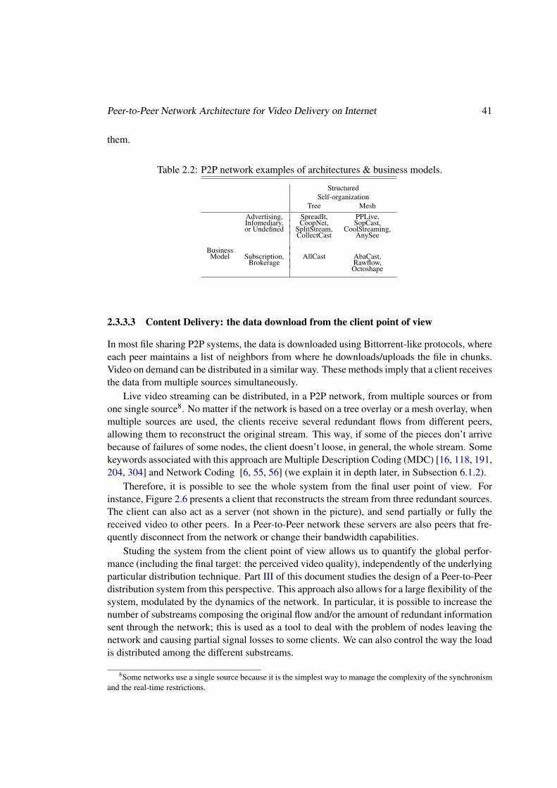
Peer-to-Peer Network Architecture for Video Delivery on Internet 41
them.
Table 2.2: P2P network examples of architectures & business models.
StructuredSelf-organization
Tree MeshAdvertising, SpreadIt, PPLive,Infomediary, CoopNet, SopCast,or Undefined SplitStream, CoolStreaming,
CollectCast AnySee
BusinessModel Subscription, AllCast AbaCast,
Brokerage Rawflow,Octoshape
2.3.3.3 Content Delivery: the data download from the client point of view
In most file sharing P2P systems, the data is downloaded using Bittorrent-like protocols, whereeach peer maintains a list of neighbors from where he downloads/uploads the file in chunks.Video on demand can be distributed in a similar way. These methods imply that a client receivesthe data from multiple sources simultaneously.
Live video streaming can be distributed, in a P2P network, from multiple sources or fromone single source8. No matter if the network is based on a tree overlay or a mesh overlay, whenmultiple sources are used, the clients receive several redundant flows from different peers,allowing them to reconstruct the original stream. This way, if some of the pieces don’t arrivebecause of failures of some nodes, the client doesn’t loose, in general, the whole stream. Somekeywords associated with this approach are Multiple Description Coding (MDC) [16, 118, 191,204, 304] and Network Coding [6, 55, 56] (we explain it in depth later, in Subsection 6.1.2).
Therefore, it is possible to see the whole system from the final user point of view. Forinstance, Figure 2.6 presents a client that reconstructs the stream from three redundant sources.The client can also act as a server (not shown in the picture), and send partially or fully thereceived video to other peers. In a Peer-to-Peer network these servers are also peers that fre-quently disconnect from the network or change their bandwidth capabilities.
Studing the system from the client point of view allows us to quantify the global perfor-mance (including the final target: the perceived video quality), independently of the underlyingparticular distribution technique. Part III of this document studies the design of a Peer-to-Peerdistribution system from this perspective. This approach also allows for a large flexibility of thesystem, modulated by the dynamics of the network. In particular, it is possible to increase thenumber of substreams composing the original flow and/or the amount of redundant informationsent through the network; this is used as a tool to deal with the problem of nodes leaving thenetwork and causing partial signal losses to some clients. We can also control the way the loadis distributed among the different substreams.
8Some networks use a single source because it is the simplest way to manage the complexity of the synchronismand the real-time restrictions.

42 Background
Figure 2.6: Client point of view of a streaming method with three servers.
2.3.4 Introduction to Network Robustness: an hybrid P2P approach
As said before, is possible to combine the advantages of Content Delivery Networks (CDN)architectures and Peer-to-Peer (P2P) networks in a hybrid system. The main idea is to extendthe resources available in the CDN with the efficiency of P2P delivery, keeping the high quality,security, and centralized control of the CDN.
Suppose we have a live video delivery service with a streaming encoding rate of bw =500 Kbps. We expect to have N = 100.000 simultaneous users in some popular events.Therefore, we need a total bandwidth of 50 Gbps in the network to support this service. Today,the average upstream bandwidth of residential users isBW out = 400 Kbps9. Suppose that eachuser provides 90% of its upload bandwidth to the network. With a hybrid system, we need abandwidth capacity of Nbw − 0.9NBW out = 14 Gbps. Instead, to serve the same numberof users with a traditional CDN architecture, we have to increase our bandwidth capacity in anadditional 36 Gbps, or we have to degrade the streaming quality to 140 Kbps per user.
As in the P2PTV networks, in the hybrid approach the bandwidth is dynamically allocated,reducing cost and avoiding local congestion or bottlenecks (for contents that are popular in alocal area).
Our GOL!P2P prototype for live video streaming (presented on Chapter 10) is a hybrid P2Psystem, with central control and distributed delivery. The central control maintains a simpletree-based structured P2P overlay network, while a multi–source streaming technique isused for a P2P delivery.
The robustness of this solution with respect to the resources dynamics is the most importantdesign element if we want to guarantee some level of video quality.
In the previous section we introduced the robustness concept from the client point of view.9Speed-test results from the popular http://broadbandreports.com reports an average residential U.S.
upstream bandwidth of 371 Kbps (and a downstream bandwidth of 1.9 Mbps) on May, 2007. Speed-tests are TCP-based bandwidth measurements that are conducted from well-provisioned servers distributed on Internet. Usersvoluntarily test their connection speeds, and the results are summarized, over a week, based on DNS domain namesor ISPs.
Search Caching: an approach for discovery scalability in Content Networks 43
In this section we extend the robustness concept with the network point of view. This introduc-tion must help to understand the rest of the document. Our design mitigates the impact of thepeer’ disconnection in two levels. In the long term the system places the peers most committedto the network (those with largest lifetime and lowest bandwidth fluctuation) near to the broad-caster to obtain a more robust overlay topology. This dynamics is formalized as a mathematicaloptimization problem and solved in Chapter 8. In the short term, and known which peers willserve the streaming to a client, we study the best streaming technique that mitigates the peers’disconnection (Chapter 7). So, both much in the long and short terms, the explicit aim is thesame: to improve the perceived average video quality of end users.
2.3.5 Summary: Conclusions, Results and Discussion
In this section we presented the Content Delivery Networks (CDN) and the peer-to-peer (P2P)networks as particular classes of Content Networks. We showed the advantages and disadvan-tages of each architecture when they are used for video delivery on the Internet. We presentedthe state of the art of P2P network design, deepening in the video delivery case, i.e., the P2PTVnetworks. Two main designs coexist for P2PTV networks: tree-based overlays and mesh-basedoverlays. Without considering the distribution design, two factors are inalterable. First, it ispossible to see the video distribution from the client point of view, where the client receivesthe video from a set of sources, with some redundancy level, and with some failure probability.Second, it is possible to combine the good properties of the CDN architecture with the efficientP2P distribution in an hybrid system. The obtained hybrid system bring a service more scalableand robust than each architecture isolated. Our P2PTV prototype, GOL!P2P, follows this idea,with a centralized control and a tree-based overlay video distribution.
2.4 Search Caching: an approach for discovery scalability in Con-tent Networks
In the previous section (Section 2.3) we presented an overview of the content delivery mecha-nisms used in Content Networks, with an in depth study about the live video delivery. Besidesof content delivery design, other very important architectural design area is the content discov-ery.
As we have previously defined, in a content network the addressing and routing are basedon the content description, instead of on its location. This means that every content networkis actually a knowledge network, where the knowledge is the information about the location ofthe nodes where each specific content is to be found. This is meta-information, in the sense ofbeing the information about the information contents itself. The knowledge network is usuallycalled overlay topology.
An objective of the network is to be able to found the most complete possible set of nodeswhere a content is lodged. This corresponds to discovering the content location in the mosteffective and efficient possible way. There are two main strategies to discover the meta-information, namely publication and search. By publication we mean the process by whicha network node unrequestedly sends meta-information it possesses to the remaining nodes. By
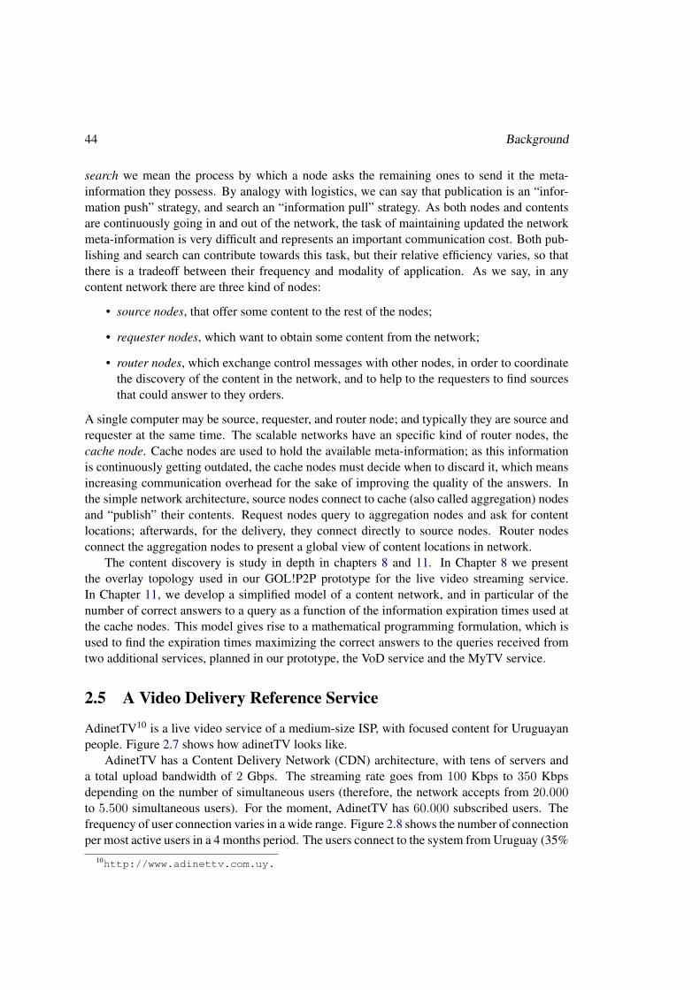
44 Background
search we mean the process by which a node asks the remaining ones to send it the meta-information they possess. By analogy with logistics, we can say that publication is an “infor-mation push” strategy, and search an “information pull” strategy. As both nodes and contentsare continuously going in and out of the network, the task of maintaining updated the networkmeta-information is very difficult and represents an important communication cost. Both pub-lishing and search can contribute towards this task, but their relative efficiency varies, so thatthere is a tradeoff between their frequency and modality of application. As we say, in anycontent network there are three kind of nodes:
• source nodes, that offer some content to the rest of the nodes;
• requester nodes, which want to obtain some content from the network;
• router nodes, which exchange control messages with other nodes, in order to coordinatethe discovery of the content in the network, and to help to the requesters to find sourcesthat could answer to they orders.
A single computer may be source, requester, and router node; and typically they are source andrequester at the same time. The scalable networks have an specific kind of router nodes, thecache node. Cache nodes are used to hold the available meta-information; as this informationis continuously getting outdated, the cache nodes must decide when to discard it, which meansincreasing communication overhead for the sake of improving the quality of the answers. Inthe simple network architecture, source nodes connect to cache (also called aggregation) nodesand “publish” their contents. Request nodes query to aggregation nodes and ask for contentlocations; afterwards, for the delivery, they connect directly to source nodes. Router nodesconnect the aggregation nodes to present a global view of content locations in network.
The content discovery is study in depth in chapters 8 and 11. In Chapter 8 we presentthe overlay topology used in our GOL!P2P prototype for the live video streaming service.In Chapter 11, we develop a simplified model of a content network, and in particular of thenumber of correct answers to a query as a function of the information expiration times used atthe cache nodes. This model gives rise to a mathematical programming formulation, which isused to find the expiration times maximizing the correct answers to the queries received fromtwo additional services, planned in our prototype, the VoD service and the MyTV service.
2.5 A Video Delivery Reference Service
AdinetTV10 is a live video service of a medium-size ISP, with focused content for Uruguayanpeople. Figure 2.7 shows how adinetTV looks like.
AdinetTV has a Content Delivery Network (CDN) architecture, with tens of servers anda total upload bandwidth of 2 Gbps. The streaming rate goes from 100 Kbps to 350 Kbpsdepending on the number of simultaneous users (therefore, the network accepts from 20.000to 5.500 simultaneous users). For the moment, AdinetTV has 60.000 subscribed users. Thefrequency of user connection varies in a wide range. Figure 2.8 shows the number of connectionper most active users in a 4 months period. The users connect to the system from Uruguay (35%
10http://www.adinettv.com.uy.

A Video Delivery Reference Service 45
Figure 2.7: AdinetTV: our video delivery reference service to design GOL!P2P.
1
10
100
1000
10000
0 5000 10000 15000 20000 25000
conn
ectio
ns
user
Number of Connections per User
Figure 2.8: Number of connection per user, in a 4 months period. Real data of a live-videodelivery reference service from a medium-size ISP. Only the 25.000 more active users areshown.
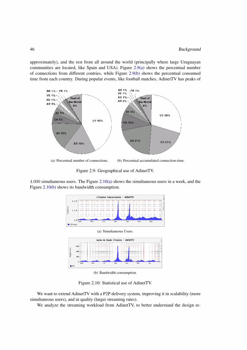
46 Background
approximately), and the rest from all around the world (principally where large Uruguayancommunities are located, like Spain and USA). Figure 2.9(a) shows the percentual numberof connections from different contries, while Figure 2.9(b) shows the percentual consumedtime from each country. During popular events, like football matches, AdinetTV has peaks of
(a) Percentual number of connections. (b) Percentual accumulated connection-time.
Figure 2.9: Geographical use of AdinetTV.
4.000 simultaneous users. The Figure 2.10(a) shows the simultaneous users in a week, and theFigure 2.10(b) shows its bandwidth consumption.
(a) Simultaneous Users.
(b) Bandwidth consumption.
Figure 2.10: Statistical use of AdinetTV.
We want to extend AdinetTV with a P2P delivery system, improving it in scalability (moresimultaneous users), and in quality (larger streaming rates).
We analyze the streaming workload from AdinetTV, to better understand the design re-
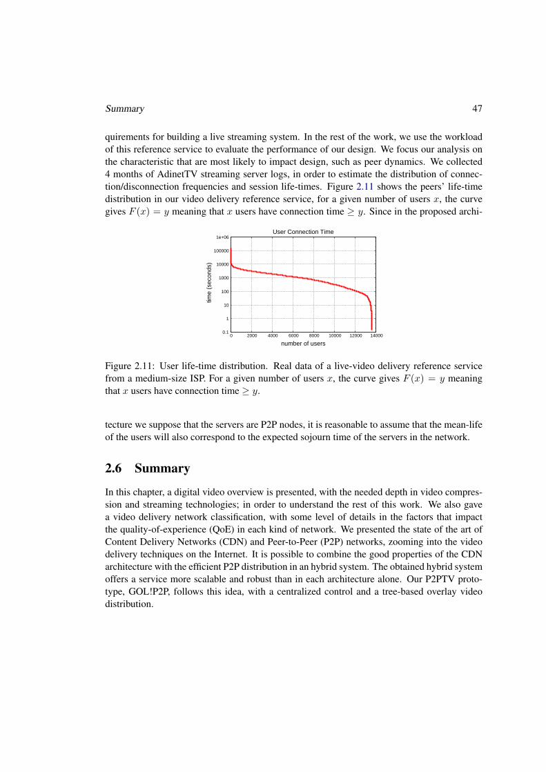
Summary 47
quirements for building a live streaming system. In the rest of the work, we use the workloadof this reference service to evaluate the performance of our design. We focus our analysis onthe characteristic that are most likely to impact design, such as peer dynamics. We collected4 months of AdinetTV streaming server logs, in order to estimate the distribution of connec-tion/disconnection frequencies and session life-times. Figure 2.11 shows the peers’ life-timedistribution in our video delivery reference service, for a given number of users x, the curvegives F (x) = y meaning that x users have connection time ≥ y. Since in the proposed archi-
0.1
1
10
100
1000
10000
100000
1e+06
0 2000 4000 6000 8000 10000 12000 14000
time
(sec
onds
)
number of users
User Connection Time
Figure 2.11: User life-time distribution. Real data of a live-video delivery reference servicefrom a medium-size ISP. For a given number of users x, the curve gives F (x) = y meaningthat x users have connection time ≥ y.
tecture we suppose that the servers are P2P nodes, it is reasonable to assume that the mean-lifeof the users will also correspond to the expected sojourn time of the servers in the network.
2.6 Summary
In this chapter, a digital video overview is presented, with the needed depth in video compres-sion and streaming technologies; in order to understand the rest of this work. We also gavea video delivery network classification, with some level of details in the factors that impactthe quality-of-experience (QoE) in each kind of network. We presented the state of the art ofContent Delivery Networks (CDN) and Peer-to-Peer (P2P) networks, zooming into the videodelivery techniques on the Internet. It is possible to combine the good properties of the CDNarchitecture with the efficient P2P distribution in an hybrid system. The obtained hybrid systemoffers a service more scalable and robust than in each architecture alone. Our P2PTV proto-type, GOL!P2P, follows this idea, with a centralized control and a tree-based overlay videodistribution.

48 Background

Part II
QUALITY
49


Chapter 3
Video Quality Assessment: State of theart
In this chapter we present the issues associated with the assessment of the quality of videostreams. We discuss the evaluation mechanisms currently available in the literature, and whythey don’t necessarily fulfill the current needs in terms of perceived quality assessment.
There are two main approaches for measuring the video quality: subjective assessment andobjective assessment. In brief, subjective assessments consist of a panel of human beings ratinga series of short video sequences according to their own personal view about quality. Objectiveassessments stand for the use of algorithms and formulas that measure the quality in a auto-matic, quantitative and repeatable way.
The rest of the chapter is organized as follows. In Section 3.1, we describe several subjec-tive quality methods and we compare the most important aspects of them. In Section 3.2, weprovide a general description of objective quality metrics. Mitigating the disadvantages of bothapproaches, hybrid methods have been developed. In Section 3.3 we present the precedentsof the PSQA methodology, that will be explained in depth in Chapter 4. Finally we provideconclusions of this chapter in Section 3.4
3.1 Subjective Quality Assessment
There is no better indicator of video quality than the one given by human observers, becausethe video is created to be watched by human beings. Unfortunately, the quality given by anobserver depends on his/her own experience. That is why we call this view the perceivedquality of the video.
Perceived video quality is, by definition, a subjective concept. The mechanism used forassessing it is called subjective testing. There are several types of subjective assessment tech-niques, which depend of the quality aspects that are evaluated and the kind of application.Two main classes of subjective assessment can be found, namely qualitative assessment, andquantitative assessment.
Qualitative assessment [36, 37] produces descriptions of an observer quality perception,
51

52 Video Quality Assessment: State of the art
and usually it does not translate well into numeric scales. This approach is useful in severalcontexts, for instance, to describe how different observers react to variations of the perceivedquality, and to evaluate the interest in proposing pricing schemes for a multimedia service.These methods are suitable to explain the “sociologic” aspects of the quality rather than to beused in an engineering design.
On the other hand, quantitative assessment provides a more concise approach to qualityassessment, and is more suitable for our work. It consists of building a panel with real humansubjects which will evaluate a series of short video sequences according to their own personalview about quality. An alternative is to use a (smaller) panel of experts. In the first case, we willget the quality of the sequences as seen by an average observer. In the second case, we can havea more pessimistic (or optimistic, if useful) evaluation. The output of these tests is typicallygiven as a Mean Opinion Score (MOS) [171]. Obviously, these tests are very time-consumingand expensive in manpower, which makes them hard to repeat often. And, of course, theycannot be a part of an automatic process (for example, for analyzing a live stream in real time,for controlling purposes).
There are standard methods for conducting subjective video quality evaluations, such asthe ITU-R BT.500-11 [171]. Some variants included in this standard are1:
• Single Stimulus (SS),
• Double Stimulus Impairment Scale (DSIS),
• Double Stimulus Continuous Quality Scale (DSCQS),
• Single Stimulus Continuous Quality Evaluation (SSCQE),
• Simultaneous Double Stimulus for Continuous Evaluation (SDSCE)
• and Stimulus Comparison Adjectival Categorical Judgement (SCACJ).
The differences between them are minimal and mainly depend on the particular applicationconsidered. They concern, for instance, the fact that in the tests the observer is shown pre-evaluated sequences for reference (which in turn, can be explicit or hidden), the quality evalu-ation scale (and the fact that it is discrete or continuous), the sequence length (usually aroundten seconds), the number of videos per trial (once, twice in succession or twice simultane-ously), the possibility to change the previously given values or not, the number of observersper display, the kind of display, etc.
In the following we shortly present and discuss some of these methods.
3.1.1 Single Stimulus (SS)
The Single Stimulus (SS) method of ITU-R BT.500-11 is also called Absolute Category Rating(ACR) in ITU-T Recommendation P.910 [174].
This method is designed to make an absolute quality assessment of audiovisual sequences.The duration of each sequence should be about 10 seconds. A gray scene (not longer than
1There are a set of ITU standards for other applications, such as ITU-T P.800 [173] for voice and ITU-TP.920 [175] for interactive multimedia.

Subjective Quality Assessment 53
500 ms) should be used at the beginning and at the end of each sequence to make it morenatural. Also, the termination of a sequence should not cause an incomplete scene, and audioand video must be perfectly synchronized. After viewing a sequence, subjects are asked to ratethe quality in a period that should be less than or equal to 10 seconds; this phase is called thevoting time. The test sequences are presented one at a time and are rated independently on anabsolute scale. There are different scales suggested in the standard, depending on the accuracyneeded; the five–point scale (Figure 3.1(a)) is the most used scale in audio tests, whereas invideo tests a more discriminative measure is required and a nine-point scale or eleven-pointscale may be used as shown in Figures 3.1(d) and 3.1(e).
Depending on the accuracy needed, the number of subjects required by the standard varyfrom 4 to 40. They should not be experts in video quality and should not have work experiencein this topic. Also they have to have normal vision. In our work we did a set of subjective testsbased in the SS method with the eleven–point scale. For more details about how to carry outthis subjective test see section 4.4.
(a) 5–point scale. (b) 5–point impairment scale. (c) 7–point comparingscale.
(d) 9–point scale. (e) 11–point scale. (f) continuousscale.
(g) double continu-ous scale.
Figure 3.1: ITU standard scales for subjective test methods.
3.1.2 Double Stimulus Impairment Scale (DSIS)
The Double Stimulus Impairment Scale o Degradation Category Rating (DSIS) method of ITU-R BT.500-11 is also called Degradation Category Rating (DCR) in ITU-T RecommendationP.910 [174].
This method is designed to measure the quality degradation caused by some encoding ortransmission scheme. The sequences are shown consequently in pairs: the first one is thereference sequence, the second one is the impaired sequence. The subjects are informed about

54 Video Quality Assessment: State of the art
which one is the reference high quality video, and are asked to rate the quality of the latter withrespect to the former using the scale shown in Figure 3.1(b) (the scales used in SS method canalso be used by replacing the quality adjectives by the corresponding impairment adjectives).The time between the reference and the impaired sequence should be less than 2 seconds, andthe voting time should be less than or equal to 10 seconds.
3.1.3 Double Stimulus Continuous Quality Scale (DSCQS)
The Double Stimulus Continuous Quality Scale (DSCQS) is designed to measure the qualitywhen the sequences only explore a sub-range of the full available range. In this situation adouble stimulus is needed to help the subjects in comparing different qualities. Sequences areplayed in pairs simultaneously2, one of the videos is the reference and the other one is theimpaired. Subjects do not know which is the reference one, and the order is changed randomlyfrom one pair to the next one. For each pair, subjects have to mark the quality of each sequencein a continuous vertical scale (Figure 3.1(g)).
3.1.4 Other Works in Subjective Video Quality Measures
Three other methods are presented in ITU-R BT.500-11. They are: Single Stimulus Contin-uous Quality Evaluation (SSCQE), Simultaneous Double Stimulus for Continuous Evaluation(SDSCE), and Stimulus Comparison Adjectival Categorical Judgement (SCACJ).
SSCQE is designed to measure the quality in a variable context, for example when anadaptative compression is used. Previously described methods measure the quality of a wholesequence, whereas SSCQE uses a continuous assessment. Where each subject constantly mea-sures the quality with the Figure 3.1(f) scale, the average score is obtained estimating theprobability distribution of each assessment.
Similar to DSCQS, SDSCE method measures two sequences simultaneously. The subjectsare requested to check the impairment between the two sequences constantly, using the 3.1(f)scale (where 100 points mean identical sequences).
Similar to the DSCQS, in SCACJ two sequences are played simultaneously, and after play-back the subject is asked to give his opinion using the comparison scale of Figure 3.1(c).
The ITU-R draft document 6Q/57-E [170] specifies the Subjective Assessment Methodol-ogy for VIdeo Quality (SAMVIQ). SAMVIQ is designed to evaluate the quality of multimediain the Internet, especially video formats and streaming techniques. SAMVIQ allows partic-ular codecs and resolutions that previous Recommendations (ITU-R BT.500) do not considerbecause were developed for TV application.
Sequences are present in multi-stimulus form. The subjects can choose the tests order andcorrect their votes. Hidden references can be used among the sequences, not only at the begin-ning of the test.
2Sometimes for simplification, the two sequences are showed in the same playback windows, given the possi-bility to freely switch between the two videos.
Subjective Quality Assessment 55
In the “Architecture and Transport” working group of the DSL Forum [86], there is a guideto implementing a test plan and to the use of video quality subjective testing with MOS Scor-ing in the IPTV context (working progress document WT-126 “Triple-play Services Quality ofExperience (QoE) Requirements and Mechanisms” [87]). In this area, accurate video-qualitymeasurement and monitoring is today an important requirement of industry. In chapter 9 wepresent an architecture to measure automatically and in real time the QoE in Video DeliveryNetworks (and particulary in IPTV systems).
Coming from the academic or the industry sector, some groups study specifically the as-sessment of subjective video quality. Some of the most important ones are the Video QualityExperts Group (VQEG) [333], the Institute für Rundfunktechnik [164], and the Graphics &Media laboratory of Computer Science department of MSU [120]. Part of this Section is in-spired by their works.
3.1.5 Subjective Test Comparison
The presented Subjective quality assessment methods principally differ in their objectives. Sin-gle Stimulus (SS) is designed to make an absolute quality assessment of audiovisual content. Tomeasure the quality degradation caused by some encoding or transmission scheme the DoubleStimulus Impairment Scale (DSIS) is more suitable. The Double Stimulus Continuous QualityScale (DSCQS) can measure the quality when the sequences only explore a sub-range of thefull available range. Single Stimulus Continuous Quality Evaluation (SSCQE) is designed tomeasure the quality in a variable context, for example when an adaptative compression schemeis used. Simultaneous Double Stimulus for Continuous Evaluation (SDSCE) checks the im-pairment between two sequences, and Stimulus Comparison Adjectival Categorical Judgement(SCACJ) compares two sequences that are played simultaneously. Closer to our applicationthere are: the Subjective Assessment Methodology for VIdeo Quality (SAMVIQ) designed toevaluate the quality of multimedia in the Internet, and the work-in progress document WT-126 “Triple-play Services Quality of Experience (QoE) Requirements and Mechanisms” of theDSL Forum, to measure QoE in IPTV networks. Based on [194], Table 3.1 summarizes themain differences between subjective test methods.
All the presented subjective quality assessment methods measure directly the perceivedquality from the user’s perspective. However, subjective tests are very time-consuming andexpensive in manpower, which makes them hard to repeat often. Furthermore, given theirnature, they are obviously not suitable for real-time operation (which is our final goal in thiswork). Moreover, the standards (except the draft SAMVIQ [170]) are designed for broadcastTV application, and they do not fit well with multimedia streaming in a best–effort network,like the Internet. In this sense, they do not fit well to our application because: they weredesigned for applications which normally have better quality levels [344, 345], with the use ofshort samples, separating audio and video, it is not possible to capture the relative importanceof video and audio in the overall quality [125, 327], and they have numerous strict parametersranging from room size to equipment calibration that make the test more expensive.

56 Video Quality Assessment: State of the art
Table 3.1: Subjective Test Comparison.
Parameter SS DSIS DSCQS SSCQE SDSCE SAMVIQITU-R Standard BT.500 BT.500 BT.500 BT.500 BT.500 BT.700
Scale discrete discrete continuous continuous continuous continuous(Figure) 3.1(a), 3.1(b) 3.1(g) 3.1(g) 3.1(g) 3.1(g)
3.1(d) or3.1(e)
Sequence 10 seg 10 seg 10 seg ≥ 5 min 10 seg 10 segLength
Reference no explicit hidden no explicit explicitand hidden
High anchor no no yes no no hiddenLow anchor no no yes no no yes
2 simultaneous no no no no yes nostimulus
Presentation once once or twice in once once severalof twice in in concurrent
sequences succession succession (multi stimuli)Possibility no no no no no yesto changethe votebefore
proceeding
3.2 Objective Quality Assessment
Considering the bad properties of subjective testing (principally those associated with the factthat they rely on the work of panels of users), researchers and engineers had naturally looked forautomatic procedures, called objective methods. Objective metrics are algorithms and formulas(generally signal processing algorithms) that measure, in a certain way, the quality of a stream.With a few exceptions, objective metrics propose different ways of comparing the receivedsample with the original one3, typically by computing a sort of distance between both signals.So, it is not possible to use them in an real–time test environment, because the received and theoriginal video are needed at the same time in the same place. But the most important problemwith these quality metrics is that they often provide assessments that do not correlate well withhuman perception, and thus their use as a replacement of subjective tests is limited.
The most commonly used objective measures for video are:
• Peek Signal to Noise Ratio (PSNR),
• ITS’ Video Quality Metric (VQM) [21, 338],
• EPFL’s Moving Picture Quality Metric (MPQM),
• Color Moving Picture Quality Metric (CMPQM) [328, 329],
• Normalization Video Fidelity Metric (NVFM) [329].
They differ in complexity, from the simplest one (PSNR) to the most sophisticated one basedon the Human Vision System (HVS) (CMPQM or NVFM). Based on previous work [218, 271],in what follows we present some of the most common objective tests.
3In audio, the E–model [172] standard specify an objective quality measurement that does not need the originalsignal; we doesn’t know a equivalent procedure for video.

Objective Quality Assessment 57
3.2.1 Peak Signal–to–Noise Ratio (PSNR)
The most common and simple objective video quality assessment is the Peak Signal–to–NoiseRatio (PSNR). We can define the Mean Square Error (MSE) between a original video sequenceo and the distorted sequence d as:
MSE =1
K.M.N
K∑k=1
M∑m=1
N∑n=1
[ok(m,n)− dk(m,n)]
where each video sequence has K frames of M ×N pixels each, and ok(m,n) and dk(m,n)are the luminance pixels in position (m,n) in the kth frame of each sequences.
The PSNR is the logarithmic ratio between the maximum value of a signal and the back-ground noise (MSE). If the maximal luminance value in the frame is L (when the pixels arerepresented using 8 bits per sample, L = 255) then:
PSNR = 10. log10
L2
MSE
An extension to color video sequences has been proposed, by considering also the chromi-nance. The first advantage of PSNR is that it is easy to compute. However, it is not appropriatein our QoE context since it does not correlate well with perceptual quality measures [26].
3.2.2 ITS’ Video Quality Metric (VQM)
ITS’ Video Quality Metric (VQM) [21, 338] is developed by the “Institute for Telecommuni-cation Sciences” (ITS). First it extracts some features from both the original and the distortedsequences. The features are an objective measure that characterizes perceptual changes of thesequence, analyzing spatial, temporal, and chrominance information. Then, a set of qualityparameters are computed comparing the original and distorted features. Using these parame-ters, a classification assigns a global quality measure. The classification is a linear combinationcalculated using functions that model human visual masking. These impairments are then sta-tistically pooled to obtain a single quality measure for the total sequence.
Summarizing, VQM makes a comparison between the original and distorted sequencesbased only on a set of features extracted independently from each video. It is useful when isnot possible to have the original and received sequences at the same time, for instance in anetwork. But it still need some information about both sequences.
VQM is accepted as an objective video quality standard by ANSI, and some studies showsa good correlation with subjective tests for low bitrate encodings (while it not performs wellfor encodings with high bitrates [26]).
3.2.3 Moving Picture Quality Metric (MPQM) and Color Moving Picture Qual-ity Metric (CMPQM)
Moving Picture Quality Metric (MPQM) [26, 329] and its color extension, Color MovingPicture Quality Metric (CMPQM) [328, 329], were developed by researchers working at the“École Polytechnique Fédérale de Lausanne” (EPFL). They are the most used objective metrics

58 Video Quality Assessment: State of the art
based on the Human Vision System (HVS) model. Stimuli of the same amplitude are perceiveddifferent when they are included in flat spatial areas or in areas including edges. In general,Stimuli with different spatial and temporal frequencies are not perceived in the same way bythe human eye. The HVS models these and other aspects of human visual perception, and it isincluded on the MPQM metric (and on the CMPQM metric) to improve his (their) performanceand robustness. In particular, MPQM incorporates the most important human perception phe-nomenon: contrast sensitivity and masking. These phenomenons accounts for the fact that aminimal threshold is needed to detect a signal change, and the threshold depends on the contrastof the foreground/background relation.
MPQM considers a set of distorted perceptual components obtained from the original se-quence and their difference with the distorted one. Each perceptual component is computedusing signal processing filters, and they measure in some way the perceptual differences be-tween the original sequence and the distorted sequence. Each component has a sensitivity in theperceptual quality, considering its weight, a global distortion E is computed (as an importantimprovement of the MSE in the PSNR metric). Finally a Masked PSNR is defined:
MPSNR = 10 log10
L2
E2
CMPQM is an extension to MPQM that also use the chrominance values. At first step ittransforms the original and the distorted sequences to the linear opponent-color space (B/W,R/G, B/Y). The computation follows in a very similar way then for the original MPQM.
The authors of these proposals show that both metrics, MPQM and CMPQM, correlatewell with subjective assessment in particular scenarios [329], specially for high bit rate codifi-cations. However, in more general situation, the correlation is more variable.
3.2.4 Normalization Video Fidelity Metric (NVFM)
Normalization Video Fidelity Metric (NVFM) [329], also developed by EPFL, is based on avisibility prediction followed by a normalization stage. As MPQM, the prediction is made inthe pixel domain, using space and time linear transformations, but is applied to the originalsequence and in the distorted sequence (instead to its difference as in MPQM). The perceptualcomponents obtained in the prediction stage are normalized based on the ratio between the ex-citatory and inhibitory of a inter–channel masking that consider the sensitivity weight. Finally,the measure metric is computed as the squared vector sum of the difference of the normalizedresponses.
3.2.5 Other Works in Objective Video Quality Measures and Comparison
Structural Similarity Index (SSIM) [342, 343] is a structural distortion based technique. Allthe previously described methods are error based. Instead, HVS is not oriented towards thatextracting structural information from the viewing field. Therefore, a measurement of structuraldistortion should be a good approximation of perceived image distortion. Only studied by itsauthors, it is not clear yet the correlation with subjective tests of this approach.

An Hybrid Quality Assessment approach: Pseudo-Subjective Quality Assessment 59
Noise Quality Measure (NQM) [77, 341] models the error source with a linear frequencydistortion and additive noise injection; the two sources are considered independent. A dis-tortion measure (DM) is used for the effect of the frequency distortion, and a noise qualitymeasure (NQM) is used for the effect of the additive noise. A global perceptual quality basedon the two measures (NQM and DM) is not defined.
Table 3.2 summarizes the considered objective metrics. Observe that all objective videoquality metrics use the original video sequence (and the distorted video sequence). There-fore, it is not possible to use them in an real–time test environment, because the received andthe original video are needed at the same time in the same place. Also in some applicationsthe complex computations involved are a limitation to their use. But the most important dis-advantage of these metrics is that they often provide assessments that do not correlate wellwith human perception. As IRT [164] says: “despite efforts to develop objective measuringmethods, the results repeatedly fail to reflect quality as perceived by the human eye, whichis uninterested in purely logical approaches. Subjective tests are therefore recommended forchecking the quality of digital videos”.
Table 3.2: Objective Metric Comparison.
Parameter PSNR VQM MPQMS CMPQM NVFM SSIMUse of Original yes yes yes yes yes yes
SequenceChrominance no yes no yes yes yesConsiderationMathematical simple very complex complex complex complex
complexity complexCorrelation with poor good varying varying varying unknown
Subjective Methods
3.3 An Hybrid Quality Assessment approach: Pseudo-SubjectiveQuality Assessment
In next chapter we present a hybrid approach between subjective and objective evaluation calledPseudo Subjective Quality Assessment (PSQA) [221]. It is a technique allowing to approximatethe value obtained from a subjective test in an automatically way. Therefore, it puts togetherthe advantages of both approaches: it allows an automatic and simple measurement at a verylow cost, and it does not need the original sequence. As a consequence, it is ideal for real–timeapplications (and for our project).
The idea is to have several distorted samples evaluated subjectively by a panel of humanobservers, and then to use the results of this evaluation to train a specific learning tool (inPSQA the best results come from the Random Neural Networks one [100]) in order to capturethe relation between the parameters that cause the distortion and the perceived quality. It isnecessary to understand that, in general, the distorted sequences used in the test phase are gen-erated for a given application, and therefore a new PSQA module must be generated for everynew application.
60 Video Quality Assessment: State of the art
The PSQA assessment approach is proposed in [218]. The authors studied its applicabil-ity to different contexts, their work principally concentrates in speech quality assessment [219,220], but also he studied the video quality [221, 222], specially for the standard video-conferencecodec H.263 [177]. In video, that is our focus, the methodology produces good evaluations fora wide range variation of all the quality affecting parameters; the published works presentevaluations with correlation coefficients with values coming from human observers up to 0.97.To use the new technique, he designed a new rate control mechanism [220]. This mecha-nism combines an automated real–time multimedia quality assessment with a TCP–friendlyrate controller, with the objective of deliver the best multimedia quality and save bandwidthconsumption.
A previous inspiring work [237] used Artificial Neural Networks to estimate audio qualityfrom signal factors (PSQA’ authors work approach analyze application and network–level fac-tors instead).
Following the first study, the PSQA’s performance was studied in–depth in the Voice overIP context [271]. This work helped to validate the methodology itself and to compare it withother quality assessment techniques [67, 223, 224, 295]. The authors studied one–way and in-teractive VoIP applications, in wired and wireless networks. They also used PSQA to evaluatedifferent redundant schemes, specially Forward Error Correction (FEC) [293]. With respectto the use of PSQA in control application, they presented a very simple priority scheme forpackets in a wireless link [294, 296].
The PSQA methodology was also applied to control a DiffServ IP network in order toimprove the performance of multimedia services [323]. This study worked at router’s levelin two main research areas: Active Queue Management (AQM) for Assured Forwarding andDiffServ-aware video streaming.
The main target of our work is a peer–to–peer prototype for live video streaming. In thenext chapter we extend PSQA to use it in this context. We improve the methodology in differ-ent ways. First, we study the effects of several parameters on the perceived video quality, inparticular the frame loss effect, instead of packet lost (studied in all previous works). Second,the influence of source’ motion in the quality is considered. And third, we analyze the impactof server failures in perceived quality. We use the PSQA quality assessment: to optimize amulti-source streaming technique with respect to server failures behavior (Chapter 6), to im-plement a robust structured overlay peer-to-peer based on quality guarantees (Chapter 8), and tomeasure and to monitor the quality in a general Video Delivery Network (VDN) automatically(Chapter 9).
3.4 Summary
In this chapter we presented the state of the art in video quality assessment. Several subjectivemethods and objective metrics are explained and compared. It is clear from this summarythat current quality assessment methods (subjective and objective) are not able to measure the

Summary 61
quality in real–time (by definition, in the subjective case, and due to the need of the originalvideo, in the objective one), disabling its use to monitoring and to controlling purposes.
Subjective tests are expensive and not suitable for real–time operation because they need atest campaign. Also, objective metrics are not suitable for real–time applications because theyneed the original an the distorted sequences at the same time to compute the metric. Moreover,they often provide assessments that do not correlate well with human perception.
The hybrid quality assessment approach, Pseudo-Subjective Quality Assessment (PSQA),adapts very well to our needs to measure in real–time the subjective video quality of a livevideo distribution system. The PSQA methodology will be explained in–depth in next chapter.

62 Video Quality Assessment: State of the art

Chapter 4
PSQA – Pseudo–Subjective QualityAssessment
The main target of our work is a quality-centric design of a peer–to–peer prototype for livevideo streaming. To measure and to control the network we use the Pseudo–Subjective Qual-ity Assessment (PSQA) methodology1. In this chapter we present the PSQA methodology(Sections 4.3, 4.4, and 4.5). In Chapter 5, we explore the sensivity of the perceived video qual-ity with respect to several quality–affecting parameters and obtain some mapping function ofquality that will be used in the rest of this work.
4.1 Overview of the PSQA Methodology
Let us briefly describe the way PSQA works. We start by choosing the parameters we thinkwill have an impact on quality. This depends on the application considered, the type of net-work, etc. Then, we must build a testbed allowing us to send a video sequence while freelycontrolling simultaneously the whole set of chosen parameters. This can be a non-trivial task,especially if we use a fine representation of the loss process. We then choose some repre-sentative video sequences (again, depending on the type of network and application), and wesend them using the testbed, by changing the values of the different selected parameters. Weobtain many copies of each original sequence, each associated with a combination of valuesfor the parameters, obviously with variable quality. The received sequences must be evaluatedby a panel of human observers using some subjective testing procedure. Each human observerevaluates many sequences and each sequence is evaluated by all the observers (as specified byan appropriate test subjective norm). After this subjective evaluation, we perform a statisticalfiltering process to this evaluation data, to detect (and eliminate, if necessary) the bad observersin the panel (a bad observer is defined as being in strong disagreement with the majority). Allthese concepts have well defined statistical meanings. At that stage enters the training process,which allows learning the mapping Q() from the values of the set of parameters into perceived
1Current video quality assessment methods are not able to measure the quality in real–time disabling its use tomonitoring and to controlling purposes (see previous chapter for details).
63

64 PSQA – Pseudo–Subjective Quality Assessment
quality. To train, we use the Random Neural Networks learning tool [100], that shows the bestsuccess results [292].
Figure 4.1 represents graphically the whole process.
Figure 4.1: Training PSQA method.
After the training phase, PSQA is very easy to use: we need to evaluate the values of thechosen parameters at time t (that is, to measure them), and then to put them into the functionQ() to obtain the instantaneous perceived quality at t. See Figure 4.2 where we representPSQA in operation.
Figure 4.2: Using PSQA method.
Summarizing, we can divide the PSQA methodology in three main stages:
• (i) the election of the parameters that we think will have an impact on quality (Sec-tion 4.3);
• (ii) the evaluation of these parameters by means of subjective tests campaign (Sec-tion 4.4);
• (iii) and finally the training process, which allows to learn the mapping from the values ofthe set of parameters into perceived quality obtained in the tests campaign (Section 4.5).
Let us now introduce some notation before describing the methodology in–depth.
A Formal Notation 65
4.2 A Formal Notation
Following previous work, we use the following formal notation to reference the principal as-pects of PSQA.
The set of a priori quality-affecting parameters are denoted by P = {π1, · · · , πP }. Theparameter πi can take a discrete set of possible values {pi1, · · · , piHi}, with pi1 < pi2 < · · · <piHi . A configuration ~v vector is defined as a vector of possible values for each parameter:~v = (v1, · · · , vp), where vi ∈ {pi1, · · · , piHi}.
The total number of possible configurations is then∏Pi=1Hi. The possible configura-
tion space is usually large, we select a subset of configurations for the testing phase, S ={~v1, · · · , ~vS}, where ~vs = (vs1, · · · , vsP ) and vsp being the value of parameter πp in configu-ration ~vs.
In a testbed environment, we generate a distorted video sequence σs, applying the ~vs param-eters conditions to an original sequence σ. Therefore, we build a test set T = {σ1, · · · , σS}of distorted video sequences, that correspond to the result of sending S-times σ through thesource-network system for the selected configurations S.
The test set T is subjectively evaluated by a panel of human users following some sub-jective method (see section 3.1). The average perceptual quality score, Mean Opinion Score(MOS), corresponding to sequence σs is denoted by qs, where qs ∈ Ψ, and Ψ is the scale rangeof the test (one option of the list in Figure 3.1).
The final goal of the PSQA methodology is to obtain a perceptual quality function of theparameters Q : P 7−→ Ψ, such that
(i) for any sample σs ∈ T , Q(vs1, · · · , vsP ) ≈ qs,
(ii) for any other vector of parameter values (v1, · · · , vP ), Q(v1, · · · , vP ) is close to theMOS that would be associated in a subjective evaluation with a media sample for whichthe selected parameters had those specific values v1, · · · , vP .
To approximate this function, we use an Random Neural Network (RNN) as will be de-scribed in 4.5.
4.3 Stage I: Quality–affecting factors and Distorted Video DatabaseGeneration
In the first stage, we select the quality–affecting factors that we think have an impact on quality,we also generate a distorted video database varying these parameters to be used on next stage.Figure 4.3 represents graphically the stage I.

66 PSQA – Pseudo–Subjective Quality Assessment
Figure 4.3: Stage I: PSQA method.
4.3.1 Quality–affecting Parameters Selection
There are lot of factors that influence the perceptual video quality. As observed before, theydepend, among other elements, on the specific application, the networking technology, etc. Themost important task in the methodology is to correctly identify the parameters that have mostimpact in the quality. It is thus recommended to do some preliminary in-house tests to verifythe choice.
The global quality of the method is very influenced by the parameters chosen, becausethe rest of the methodology application has to be repeated if a missing factor is detected later(it includes repeating the time–consuming subjective test campaign). The accuracy and therobustness of the measure are diminished when unrelevant parameters are chosen, because thelearning tool will not be able to mimic subjective perception since important information ismissing.
In this situation, it is logical to think that is important to incorporate the larger number ofpossible parameters. But as we will see, this implies more value combinations to be watchedand evaluated in the test campaign, and there are empirical restrictions in the number of se-quences that can be used (because the excessive time and manpower needed in the test cam-paign)2.
Following this reasoning, the number of possible values that a parameter can take hasto be carefully selected: they must have the needed granularity, but keeping the number ofconfiguration low enough, in order to have manageable size tests.
It is possible to classify the quality–affecting factors into four categories, depending on thefactor source:
• Environment parameters. Environment parameters are for example: the ambient noiselevel, the lighting of the room, the fidelity of the display (monitor or TV) and the speak-ers used, the computation power capabilities of the media player (the computer), etc.The environment parameters are usually uncontrollable, and difficult to measure in atesting session. Therefore, we will usually not consider these factors in the developedmethodology.
• Source parameters. The original source video signal has an obvious strong impact onthe global perceived quality. For example the sound level, or the luminance level, andthe average motion, have an impact in the quality, especially in conjuntion with otherfactors, like very low bit rate encoding and/or packet losses in the network.
2In all our studies (and previous work) we consider less than ten parameters.

Stage I: Quality–affecting factors and Distorted Video Database Generation 67
The video source parameters like the nature of the scene (e.g. amount of motion, color,contrast, image size, etc.) that depends on the characteristics of the particular sequencethat is being transmitted can also have an impact on the human perception of the videoquality.
The encoding or compression parameters are the most important source factors. Someof these parameters are: the type of the codec used (MPEG-2, MPEG-4 Part 2 or Part 10,etc.), the sampling rate, the number of bits per sample, the bit rate, the frame rate, theencoded frame types, the number of layers in the case of layered codecs, etc.
The sender can implement some quality–improving techniques (the receiver also hasto interpret the added or modified data). The most common one are: Forward ErrorCorrection (FEC), interleaving, layered coding, and, for us, our multi-source streamingproposal. Basically, these improving techniques are designed to mitigate the effect onthe quality of the packet losses in the network, and the server failures in the multi-sourcecase. Therefore if some parameter of these improving techniques is used, it is also nec-essary to include another parameter measuring the failure factor (i.e. the losses).
• Distribution (or network) parameters. The quality–of–service (QoS) measures at thenetwork are main components in network design and management, in general. Typically,they include packet loss, delay, jitter, and bandwidth factors, but it is not clear how muchthese factors affect the global perceived quality, and therefore which one and how theyhave to be parameterized. Even more, there are different sensitivities of the quality withrespect to the specific multimedia application. For instance, if real-time distribution isneeded, the packet loss rate is the most important network parameter, and the retrans-mission and buffering receiver factors take an important role. If there is interactivity(for example in a video call), delay and jitter have an important role also, adding echo,crosstalk and lost of audio/video synchronization that can be mitigated with receivertechniques too.
Internet is a best–effort network, meaning that there is no QoS guarantees to the users.Nevertheless, some techniques are applied to mitigate the network distribution effect onquality. For instance, Random Early Detection (RED) is an active queue managementalgorithm, applied into the routers of the network, that partially avoids congestion. Indedicated IP networks, a set of techniques are often developed to allow traffic engineer-ing, like Differentiated Services (DiffServ) and Multi Protocol Label Switching (MPLS).All this network improving quality techniques are parameterized and can be taken intoaccount.
The transport–layer protocols (i.e. Real–time Transport Protocol (RTP)) and application–layer signaling protocols (i.e. RTCP, H.323 and SIP) are important for quality also,because they can provide, in different ways, retransmission, extra synchronization infor-mation, congestion control algorithms, etc.
Overlay networking is becoming popular these days. These are virtual networks devel-oped at the application level over the Internet infrastructure. In particular, Peer–to–Peernetworks are becoming more and more popular today (they already generate most of the

68 PSQA – Pseudo–Subjective Quality Assessment
traffic in the Internet). For instance, P2P systems are very used for file sharing and distri-bution; some known examples are Bittorrent, KaZaA, eMule, etc. They use the often idlecapacity of the clients to share the distribution load. As a consequence, as the number ofcustomers increases, the same happens with the global resources of the network. Theirmain technical problem is that peers connect and disconnect with high frequencies, in anautonomous and completely asynchronous way. This means that the resources of the net-work as a whole are also highly variable, and thus, that the network must be robust faceto these fluctuations. The main idea that has been considered to deal with these problemsis to build the systems using some redundancy in the signals: it is possible to increasethe number of sources and/or the amount of redundant information sent through the net-work. This can be used as a tool to deal with the problem of nodes leaving the network(we will refer to this situation as a node failure), causing partial signal losses to someclients, and therefore a degradation of quality. In section 2.2 we study the failure factorsin the distribution in a Video Delivery Network (VDN), and in 2.3 some particularitiesof Peer–to–Peer network for video delivery.
• Receiver parameters. Besides the quality–improving techniques implemented by thesender (with the understanding of the receiver), there are a set of quality–improvingprocedures which can be implemented at the receiver alone.
Some examples are: buffering, loss concealment (insertion, interpolation and regenera-tion of lost data), and congestion control improvements in UDP streams.
Another relevant classification for the quality–affecting factors is with respect to the ab-stract layer where the measurement is made:
• Network level parameters. In IP networks, network level parameters are the typicalquality–of–service (QoS) measures: packet loss, delay, jitter, bandwidth, etc.
• Application level parameters. Some factors of the application influence the quality.The encoding used is a main one; other examples are the buffering technique, the stream-ing protocol (that uses mechanisms to mitigate the packet losses and the network con-gestion, etc), etc. A common stack protocol of video streaming is: RTP/UDP/IP. At theencoding output, the video is an Elementary Stream; after that it is divided into packets(Packetized Elementary stream); then, it is multiplexed with an audio stream (TransportStream). Finally, this Transport Stream is streaming over RTP. Therefore, also at theapplication level, there are different levels where it is possible to find relevant quality–affecting parameters.
In proprietary IP network deployments, to measure network level parameters is an easytask for operators and managers, and to measure application level ones implies an interferencein the client service. On the other hand, the network level parameters are less correlated withthe quality than the application level ones. But, less correlation does not mean less precisionin the quality assessment, it usually means less robustness with respect to some change in theenvironment factors. For example, we know that losses degradate quickly the quality, but it isnot the same to measure packet losses than frame losses. For example, at the application level,
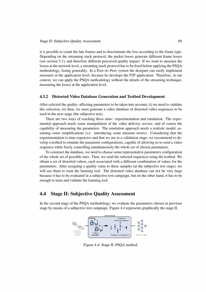
Stage II: Subjective Quality Assessment 69
it is possible to count the late frames and to discriminate the loss according to the frame type.Depending on the streaming stack protocol, the packet losses generate different frame losses(see section 5.1), and therefore different perceived quality impact. If we want to measure thelosses at the network level, a streaming stack protocol has to be fixed before applying the PSQAmethodology, losing generality. In a Peer–to–Peer system the designer can easily implementmeasures at the application level, because he develops the P2P application. Therefore, in ourcontext, we can apply the PSQA methodology without the details of the streaming technique,measuring the losses at the application level.
4.3.2 Distorted Video Database Generation and Testbed Development
After selected the quality–affecting parameters to be taken into account, (i) we need to validatethis selection, (ii) then, we must generate a video database of distorted video sequences to beused in the next stage (the subjective test).
There are two ways of reaching these aims: experimentation and emulation. The exper-imental approach needs some manipulation of the video delivery service, and of course thecapability of measuring the parameters. The emulation approach needs a realistic model, as-suming some simplifications (i.e. introducing some measure errors). Considering that theexperimentation is time expensive and that we are in a validation stage, we recommend to de-velop a testbed to emulate the parameter configurations, capable of allowing us to send a videosequence while freely controlling simultaneously the whole set of chosen parameters.
To construct the database, we need to choose some representative parameters configurationof the whole set of possible ones. Then, we send the selected sequences using the testbed. Weobtain a set of distorted videos, each associated with a different combination of values for theparameters. After assigning a quality value to these samples (at the subjective test stage), wewill use them to train the learning tool. The distorted video database can not be very largebecause it has to be evaluated in a subjective test campaign, but on the other hand, it has to beenough to train and validate the learning tool.
4.4 Stage II: Subjective Quality Assessment
In the second stage of the PSQA methodology, we evaluate the parameters chosen in previousstage by means of a subjective test campaign. Figure 4.4 represents graphically the stage II.
Figure 4.4: Stage II: PSQA method.

70 PSQA – Pseudo–Subjective Quality Assessment
4.4.1 A Subjective Test Campaign
For the subjective test campaign we can use some of the methods explained in Section3.1. Inparticular, we follow the Single Stimulus (SS) method of ITU-R BT.500-11 [171]. Briefly,some important considerations are:
• With respect to the video database and its presentation. The ITU recommends thatthe duration of each video sequence should be less than 10 seconds, without abrupttermination or incomplete meaning. Between sequences, a gray scene (not longer than500ms) can be used for a more natural presentation.
The sequence test evaluation should be divided into multiple sessions, with each sessionnot longer than 30 minutes. Each session should start with some warm–up sequences(about four or five), which should not be taken into account in the results
Some sequences with perfect quality have to be used in each session as references. Thereliability of subjects should be qualitatively evaluated by checking their votes for thereferences.
• With respect to the subjects. For statistical reasons, the number of subjects requiredto carry out the test can vary from 4 to 40, although most tests require from 10 to 20subjects. Subjects should not be experts in video quality evaluation or its theory, andthey must have normal visual acuity.
Some written instructions should be given to the subjects before carrying out the test.Also it should be necessary to show preliminary trials, to help in the explanation and tofamiliarize them with the voting scale and the task they will perform. They should notreceive any information on the quality–affecting factors that are being considered in thedatabase.
4.4.2 Mean Opinion Score (MOS) Calculation and Related Statistical Analysis
Following our formal notation (Section 4.2), the test set T = {σ1, · · · , σS} of distorted videosequences is subjectively evaluated by a human panel. Let us denote by N the number of sub-jects in the panel, and by qis the vote of sequence σs made by subject i. The average perceptualquality score or Mean Opinion Score (MOS), corresponding to sequence σs is denoted by qs,that is
qs =1N
N∑i=1
qis (4.1)
The standard deviation of this sequence σs is denoted by δs, using
δs =
√√√√ N∑i=1
(qis − qs)2N − 1
It is possible that some subjects do not follow the voting instructions, or do not pay enoughattention during the test; these subjects degradate the global precision of the PSQA method andusually they are statistical filtered in this stage.

Stage II: Subjective Quality Assessment 71
We follow the ITU-R BT.500-11 recommendation [171] for our statistical filtering. First,we use the β2 test to determine whether the votes have a normal distribution or not. Let
β2s =m4s
m22s
where mxs =1N
N∑i=1
(qis − qs)x.
If 2 ≤ β2s ≤ 4 then the votes distribution (qis)i=1,··· ,N may be assumed to be normal.Knowing that the votes have a normal distribution, it is possible to reject bad observers,
defining a bad observer as a subject such that its votes are systematicly far from the meanvotes. for each subject i we define two counters Pi and Qi following the Algorithm 1.
Algorithm 1 Statistical Filtering of β2 Test. Update rules for P and Q.Pi ← 0Qi ← 0for s = 1 to S do
if 2 ≤ β2s ≤ 4 thenif qis ≥ qs + 2× δs thenPi ← Pi + 1
end ifif qis ≤ qs − 2× δs thenQi ← Qi + 1
end ifelse
if qis ≥ qs +√
20× δs thenPi ← Pi + 1
end ifif qis ≤ qs −
√20× δs then
Qi ← Qi + 1end if
end ifend for
We can then eliminate any subject i such that
Pi +QiS
> 0.05 and∣∣∣∣Pi −QiPi +Qi
∣∣∣∣ < 0.3
The β2 test should only be run once. After this filtering, a final Mean Opinion Score (MOS)should be recomputed on the resulting subject set, using Equation 4.1. Also an average rootmean square error δ of a subject of the panel can be computed to know the variability of thepanel with respect to their quality assessment:
δ =N∑i=1
√√√√ S∑s=1
(qis − qs)2S
N(4.2)

72 PSQA – Pseudo–Subjective Quality Assessment
4.5 Stage III: Learning of the quality behavior with a RandomNeural Networks(RNN)
The result of stage II is a quality evaluation for each video sequence in the test set T . Eachdistorted video sequence is based on some parameters conditions. Therefore, the final goal ofthe PSQA methodology is to obtain a perceptual quality function of the parameters such thatthey smoothly approximate the empirical test values. To build this function, we use a RandomNeural Network (RNN). In what follows we present this learning tool. Figure 4.5 representsgraphically the stage III.
Figure 4.5: Stage III: PSQA method.
4.5.1 Random Neural Networks (RNN) overview
Random Neural Networks (RNN), also called G-networks, were proposed in [100, 101, 103]as an new type of Neural networks. They are also open Markovian queuing network with“positive” and “negative” customers (see below). Since the proposal, RNNs have been suc-cessfully applied in many areas. Its author used it in networking applications several times[70, 71, 104–106, 108, 111]. For a pretty complete survey of its applicability see [24].
The random neural network (RNN) is a simplified model of a biological nervous system.The RNN is formed by a set of neurons which exchange signals in the form of spikes, likethe natural pulsed behavior. Each neuron’s state is a non-negative integer called its potential,which increases by 1 when a positive signal (an excitation) arrives to it, and decreases by 1when a negative signal (an inhibition) arrives. The signals can originate outside the network,or they can come from other neurons. Usually, the signals can not flow in an arbitrary way: atopology is designed that specify which neurons receive signals from which ones, and whichneurons receive signals from the environment.
In our PSQA methodology, we use a particular RNN architecture, where each neuron be-haves as a ./M/1 queue with respect to positive signals. This means that positive signals areinterpreted as customers, these customers arrive to the neurons, and are served in a FIFO order.The service rate at neuron i is denoted by µi. A neuron i receives positive customers from theenvironment according to a Poisson process with rate λ+
i (no negative customers arrive fromthe environment).
The potential of a neuron is the number of positive customers in its waiting queue. Whena neuron receives a positive customer, either from another neuron or from the environment,its potential is increased by 1 (i.e. increase the waiting queue). If a neuron with a strictly

Stage III: Learning of the quality behavior with a Random Neural Networks(RNN) 73
positive potential receives a negative customer its potential decreases by 1 (i.e. a negativecustomer arrive kills the last customer at the queue (if any), and kills itself). After leavingneuron (queue) i, a customer either leaves the network with probability di, goes to queue j asa positive customer with probability p+
ij or as a negative customer with probability p−ij . So, ifthere are M neurons in the network, for all i = 1, · · · ,M :
di +M∑j=1
(p+ij + p−ij) = 1 (4.3)
At any time, the network state is specified by the potential (positive customers waitingqueue) of its neurons: ~Nt = (N1
t , · · · , NMt ), where N i
t is the potential of neuron i at time t(see Figure 4.6 for a graphical representation of a neuron in a RNN topology).
Figure 4.6: Neuron detail in a RNN.
As shown in [101, 103], if this Markov model is stable, we have, in steady-state, the fol-lowing joint probability distribution:
Pr( ~Nt = (k1, · · · , kM )) =M∏i=1
(1− %i)%kii .
Equilibrium factors %’s are the loads in the network (i.e. %i is the asymptotic probability thatqueue i is not empty).
The loads are obtained by solving the following non-linear system of equations, built interms of the individual service rates, environment arrivals and routing probabilities:
%i =
λ+i +
M∑j=1
%jw+ji
µi +M∑j=1
%iw−ij
, i = 1, · · · ,M (4.4)
The numbersw+ij = µip
+ij andw−ij = µip
−ij are called weights (as in the standard neural network
terminology).
74 PSQA – Pseudo–Subjective Quality Assessment
It can be proved that th network is stable if and only if this non-linear system (Equation 4.4)has a solution where for all i ∈ {1, · · · ,M}, %i < 1.
4.5.2 Using RNN as a function approximator: a learning tool
A common use of the RNN is as an approximator for bounded and continuous functions, in ourcontext, a learning tool. Knowing the values of a set of input (i.e. the mapping between inputsand outputs), the RNN learns how to evaluate the function for any input. The function input isthe vector ~λ = (λ+
1 , · · · , λ+M ), i.e. the environment customers arrival rate. And the function
output is the vector ~% = (%1, · · · , %M ), i.e. the stationary loads of the RNN3. As we will seenext, we usually consider that only some neurons have environment customers arrivals, and seethe output load only in some neurons (not in the whole vector ~%).
The result of stage II is a quality evaluation (MOS), qs, for each video sequence σs of thetest set T = {σ1, · · · , σS} . The distorted video sequence σs is generated in the testbed, withthe parameters conditions ~vs = (vs1, · · · , vsP ). At stage III, a perceptual quality function isapproximated using a Random Neural Network (RNN). This function, Q : P 7−→ Ψ, fromthe parameters to the perceived quality, approximates smoothly the values: (~vs, qs)s=1,··· ,S .Therefore, our RNN has:
• A single scalar output value, which corresponds to the perceived quality for any givenparameter configuration. It means that we will only consider one output neuron, o, andso the perceived quality will be given by its load %o.
• It must have P input neurons, one for each quality–affecting parameter, and the rate ofthe arrival flow (of positive customers) at neuron p is λ+
i = vp.
We need that for any sample σs ∈ T , the function approximate the empirical quality,Q(vs1, · · · , vsP ) ≈ qs. It means that if the arrival rate of each p neuron (of the P inputneurons) is λ+
i = vsp, then the occupation rate of output neuron o is %o ≈ qs. The process thatallows this adjusting is known as training, and it implies the calibration of the all weights ofthe neurons.
It is possible to consider the output %o as a function of the set of weights (denoted here by~w) and of the arrival rates ( ~λ+): %o(~w, ~λ+), and then minimize the mean square error (MSE)for the know mapping values, defined by:
MSE =1S
S∑s=1
(%o(~w, ~vs)− qs)2. (4.5)
The optimal weights values ~w0:
~w0 = argmin~w≥~012
S∑s=1
(%o(~w, ~vs)− qs)2
3Do not confuse the output of the RNN as a learning tool (the vector ~%), with the output flow of customers ofthe network. In open queuing network models, usually the output process is the flows of customers going out of thesystem (the mean rate of customers leaving the network from neuron i is %iµidi).

Stage III: Learning of the quality behavior with a Random Neural Networks(RNN) 75
can be found using a gradient–descent algorithm (as proposed by Gelenbe [102]), or with moresophisticated techniques, as the Levenberg–Marquardt method or the quasi–Newton optimiza-tion proposed by [207]. In this work we use the simple gradient descent algorithm to train theRNN.
4.5.2.1 Training and Validating
There are three major learning algorithm classes: supervised learning, unsupervised learningand reinforcement learning. Each class correspond to a particular kind of problem, the super-vised learning is used in function approximation problems4.
Usually, when working with supervised learning algorithms, the empirical database is usedto train the learning tool and also to test its performance. This means that we divide the mapping(~vs, qs)s=1,··· ,S in two parts: one is used to train the tool, and the other one is used to validateit.
If the training set is too large, it is possible that the RNN will be overtrained, i.e. thatthe performance of RNN will be very good at the training phase while it will give very poorperformance for the validating set. The performance is measured as the Mean Square Error(MSE) of the validating set. On the other hand, it is possible that the RNN will be undertrained,that is, that the training set is not large enough to extrapolate well the behavior with respect tothe values in the validating set).
Depending on the number of sequences, the number of parameters, and the values that theparameters can take, the percentage sizes of the training and validating sets are chosen. A goodstart is 80% for the training set and 20% for the validating set.
The size of training and validating sets are one of the decisions to take when a RNN is inuse. Another important decision is the RNN topology used (see below).
4.5.3 The RNN topology design
As said before, the customers can not flow in an arbitrary way, a topology is designed thatspecify which neurons receive customers from each other, and which neurons receive cus-tomers from the environment. The topology has an impact in the performance of the RNNapproximation, and has to be chosen with some care.
For the RNN there are many possible topologies: feed–forward, recurrent, etc. In ourexperiments, we use the most common one, the feed–forward, where there are no cycles orloops in the network (i.e. a customer cannot visit more than once any given queue). Theneurons, in a feed-forward network, are typically grouped in layers; where there is no edgebetween neurons at the same layer. See Figure 4.7 for a graphical representation of a typicalfeed-forward network.
4Unsupervised learning is a class of learning algorithm that not use human prepared examples to learn [131], itis used mainly in clustering and pattern recognition. Reinforcement learning is a class of learning algorithm thatattempt to find optimal actions of an agent in a particular environment. It differs from the supervised learning inthat correct input/output pairs are not explicitly presented [318].

76 PSQA – Pseudo–Subjective Quality Assessment
Some good properties of the feed–forward topology are: simple formulas and simple train-ing algorithms (see [100–103, 109] for details). In particular, the trained RNN correspondsto a rational function of its input variables; the degrees of the numerator and the denominatordepend on the number of hidden layers and the number of neurons in each.
Previous experiments [271] analyze the performance of several neural network topologies,ranged from the extremely simple two–layer design to more complex ones with several hiddenlayers and feedback between neurons. They didn’t show significant variations in performancebetween topologies, just a faster convergence of the complex ones during the training process.But the training is an off–line process that executes only once; therefore, in our experimentswe only used the two–layer and three–layer designs.
Figure 4.7: Components of a RNN. The schematics show a portion of a three–layer feed–forward network.
4.5.3.1 The simplest design: a Two–Layer RNN Topology
The two–layer topology is a feed-forward RNN, where there are P neurons receiving positivecustomers from the environment. This set of neurons is P , and is called the input layer. Eachexternal flow corresponds to one of the quality–affecting parameters, and λ+
i is the ith param-eter’s value. Typically, normalized parameters are used, i.e. λi ∈ [0, 1]. The output layer sendscustomers out of the network, it has only one neuron, denoted here by o, where we approximatethe perceptual quality (with its load %o). See Figure 4.8 for a graphical representation of thetwo–layer design.
The neuron balance equation (Equation 4.3) can be expressed in function of weights (w+ij =
µip+ij and w−ij = µip
−ij a) as:
di +1µi
M∑j=1
(w+ij + w−ij) = 1 (4.6)
For each input neuron i ∈ P there are not outputs to the environment (di = 0) and there arecustomers flows only to the output neuron o ( w+
ij = w−ij = 0 if j 6= o). Using the general
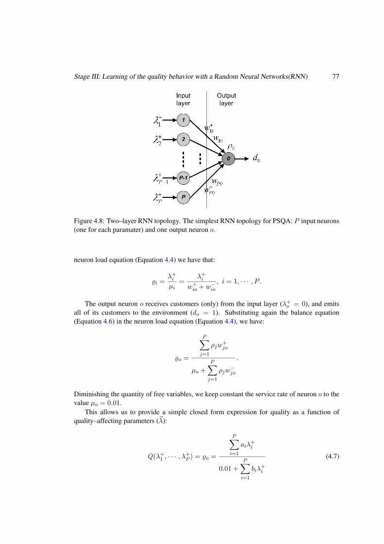
Stage III: Learning of the quality behavior with a Random Neural Networks(RNN) 77
Figure 4.8: Two–layer RNN topology. The simplest RNN topology for PSQA: P input neurons(one for each paramater) and one output neuron o.
neuron load equation (Equation 4.4) we have that:
%i =λ+i
µi=
λ+i
w+io + w−io
, i = 1, · · · , P .
The output neuron o receives customers (only) from the input layer (λ+o = 0), and emits
all of its customers to the environment (do = 1). Substituting again the balance equation(Equation 4.6) in the neuron load equation (Equation 4.4), we have:
%o =
P∑j=1
ρjw+jo
µo +P∑j=1
ρjw−jo
.
Diminishing the quantity of free variables, we keep constant the service rate of neuron o to thevalue µo = 0.01.
This allows us to provide a simple closed form expression for quality as a function ofquality–affecting parameters (~λ):
Q(λ+1 , · · · , λ+
P ) = %o =
P∑i=1
aiλ+i
0.01 +P∑i=1
biλ+i
(4.7)

78 PSQA – Pseudo–Subjective Quality Assessment
where
ai =w+io
w+io + w−io
and bi =w−io
w+io + w−io
.
This also allows to easily analyze the sensitivity of the quality with respect to a specific param-eter p. Formally, setting a0 = 0 and b0 = 0.01,
∂Q∂λ+
p=
c0 +P∑i=1
ciλ+i
(b0 +P∑i=1
biλ+i )2
where
ci =∣∣∣∣ap aibp bi
∣∣∣∣ = apbi − bpai (in particular, cp = 0).
See Section 5.2.4 for our application of the two–layer topology.
4.5.3.2 The Three–Layer RNN Topology
Extending the two–layer design, the three–layer topology adds a hidden layer between the inputlayer and the output layer. As in the two–layer topology, the input layer, P , has P neurons(one for each quality–affecting parameter) and the output layer has one neuron o (where weapproximate the perceptual quality by the output neuron load %o). Between this output neuronand the set of input neurons P , there is a set ofH neurons,H, called the hidden layer, receivingflows from the set P and sending customers to neuron o (there is no connection between P ando). See the graphical representation in Figure 4.9.
Like in the two–layer topology, the load of a neuron i ∈ P at the input layer is:
%i =λ+i
µi, i = 1, · · · , P .
The hidden layer is not directly connected to the environment, i.e. that for each neuron h ∈ H,λ+h = λ−h = dh = 0. Therefore, the load at a neuron h ∈ H is:
%h =
∑i∈P
λ+i
µiw+ih
µh +∑i∈P
λ+i
µiw−ih
,
and finally, the load at the output neuron o is:
%o =
∑h∈H
%hw+ho
µo +∑h∈H
%hw−ho
.

Stage III: Learning of the quality behavior with a Random Neural Networks(RNN) 79
Figure 4.9: Three–layer RNN topology: P input neurons (one for each paramater), H hiddenneurons, and one output neuron o.
In the training algorithm there are some restrictions over the weights to mantain the stabilityof the queueing network. To keep the network stable (∀iwe need %i < 1), a sufficient conditionis that: for any input neuron i ∈ P , λ+
i < µi; for any hidden neuron h ∈ H, µh ≥ P ; andfinally µo ≥ P in the output neuron5. Generally, these stability conditions are considered inthe training algorithm of a feed–forward network.
In the three-layer topology is possible to arbitrary adjust the number of neurons in thehidden layer, H . With a small value of H , the RNN will not learn correctly the problem. Onthe other hand, with a large value ofH , the topology will be more complex and there is a risk ofovertraining. There are some heuristic methods to find the optimal number of hidden neurons.However, they do not perform well in the general case. Instead, in our experiments, we do thefollowing:
1. Start by one hidden neuron.
2. Train this RNN topology until a minimum error goal is achieved, repeat the trainingprocess a few times and take the best one.
3. Until a maximum value is reached, increment the number of hidden neurons by one andgo to step 2.
5The same stability argument can be applied to the two–layer topology.

80 PSQA – Pseudo–Subjective Quality Assessment
4. Select the topology that gives the best performance for both the training and the testingsteps.
Usually, the trainig algorithm initializes randomly the weights, so, different executions canachieve different performance. For robustness, it is necessary to train the RNN a few times(and take the best one) for each topology (i.e. each number of hidden neurons). Also, to getthe best performance is possible to change the stopping criterion of the training process, forexample to diminish the minimum error goal or to increase the amount of iterations.
4.6 Operation Mode
After training the PSQA method (stages I, II and III), the PSQA is very easy to use. It isnecessary to measure the quality–affecting parameters at time t, and to evaluate these valueswith the Q() function (actually the RNN) to obtain the instantaneous perceived quality at t.We represent PSQA in operation in Figure 4.10
Figure 4.10: Using PSQA method.
4.7 Summary
In this chapter we presented the Pseudo–Subjective Quality Assessment (PSQA) methodology.The configuration of the PSQA method has three stages:
• Stage I. The election of the quality–affecting factors that we think will have an impacton quality. The generation of a distorted video database varying these parameters.
• Stage II. The evaluation of these parameters by means of a subjective test campaign.
• Stage III. The Random Neural Networks(RNN) training process, which allows to learnthe mapping from the values of the set of parameters into perceived quality obtained inthe test campaign.
After configuring, the PSQA is very easy to use, including to measure and to control videodelivery networks in real–time. In next chapter, we explore the sensivity of the perceived videoquality with respect to several quality–affecting parameters and obtain some mapping functionof quality that will be used in the rest of this work.

Chapter 5
Studying the Effects of SeveralParameters on the Perceived VideoQuality
In this chapter we apply the PSQA methodology (explained in Chapter 4) to use it in videodelivery networks design. In order to increase the generality of the assessment to different con-texts, we improve the PSQA methodology in three ways. First, we study the effects of severalparameters on the perceived video quality, in particular the frame loss effect, instead of packetloss (studied in all previous works). Second, we look at the influence of source motion in thequality. And third, we analyze the impact on quality of server failures.
We apply the PSQA procedure in two different scenarios: a simple one for MPEG-2 videoencoding, and a sophisticated one, that considers video source properties for MPEG-4 videoencoding. The results of these tests have been used in the core of many publications and theywill help us in the rest of our work; in particular, we use the PSQA quality assessment: to op-timize a multi-source streaming technique with respect to server failures behavior (Chapter 6),to implement a robust structured overlay peer-to-peer based on quality guarantees (Chapter 8),and to measure and to monitor the quality in a general Video Delivery Network (VDN) auto-matically (Chapter 9).
5.1 Parameters Selection: Network level or Application level?
The global quality of the PSQA methodology is very influenced by the quality–affecting factorschosen. There are a lot of factors that influence in the perceptual video quality, even if weconsider a specific application (likes our live video delivery over P2P).
The parameters have to be carefully selected: we must include the most important affectingfactors, while keeping their number reasonable (an excessive number leads more subjectivetests and complex RNN’s topologies). With our objectives, they have to be easy to measure ina real–time P2P application. For a general discussion about paramters selection see Section 4.3.
We know from previous work on PSQA that the loss process is the most important global
81
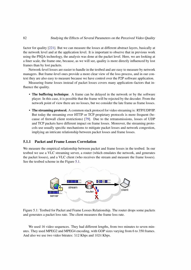
82 Studying the Effects of Several Parameters on the Perceived Video Quality
factor for quality [221]. But we can measure the losses at different abstract layers, basically atthe network level and at the application level. It is important to observe that in previous workusing the PSQA technology, the analysis was done at the packet level. Here, we are looking ata finer scale, the frame one, because, as we will see, quality is more directly influenced by lostframes than by lost packets.
Network-level losses are easier to handle in the testbed and are easy to measure by networkmanagers. But frame-level ones provide a more clear view of the loss process, and in our con-text they are also easy to measure because we have control over the P2P software application.
Measuring frame losses instead of packet losses covers many application–factors that in-fluence the quality.
• The buffering technique. A frame can be delayed in the network or by the softwareplayer. In this case, it is possible that the frame will be rejected by the decoder. From thenetwork point of view there are no losses, but we consider the late frame as frame losses.
• The streaming protocol. A common stack protocol for video streaming is: RTP/UDP/IP.But today the streaming over HTTP or TCP propietary protocols is more frequent (be-cause of firewall client restrictions) [79]. Due to the retransmissions, losses of UDPand TCP packets have different impact on frame losses. Moreover, the streaming proto-cols use usually specific mechanisms to mitigate packet losses and network congestion,implying an intricate relationship between packet losses and frame losses.
5.1.1 Packet and Frame Losses Correlation
We measure the empirical relationship between packet and frame losses in the testbed. In ourtestbed we use a VLC streaming server, a router (which emulates the network, and generatesthe packet losses), and a VLC client (who receives the stream and measure the frame losses).See the testbed scheme in the Figure 5.1.
Figure 5.1: Testbed for Packet and Frame Losses Relationship. The router drops some packetsand generates a packet loss rate. The client measures the frame loss rate.
We used 16 video sequences. They had different lengths, from two minutes to seven min-utes. They used MPEG2 and MPEG4 encoding, with GOP sizes varying from 6 to 350 frames.And also we use two video bitrates: 512 Kbps and 1024 Kbps.

Parameters Selection: Network level or Application level? 83
The VLC software admits a lot of streaming protocols: UDP, HTTP, HTTPS, RTP, RTSPand MMS (see VLC web site [334] for details). We streamed our 16 sequences over UDP andHTTP.
The streaming crosses an emulated network with some constraints in delay and bandwidth.The delay is 200 ms all over the tests, and the bandwidth depends on the encoding bitrate:for 512 Kbps of encoding bitrate we have a bandwidth of 717 Kbps, and for 1024 Kbps ofencoding bitrate we have a bandwidth of 1280 Kbps. The network also drops packets withdifferent predefined rates.
We can extract important information just looking at the average behavior of several tests.
• Encoding influence in frame losses. We streamed (using UDP and HTTP) a set of videosencoded with MPEG-2, with two bitrates (512 Kbps and 1024 Kbps), and in twentydifferent packet losses rates in the network. On the average we obtained 3.8% of packetlosses and 47.9% of frame losses. With the same streaming protocol, bitrates and packetlosses situations, we then streamed the same set of videos but this time encoded withMPEG-4. For MPEG-4 we obtain 30.2% of frame losses (there are 3.8% of packetlosses again, because we are in the same network situations). Maintaining the packetlosses, clearly the encoding standard has an important impact in the frame lossess.
• Bitrate influence in frame losses. We can observe the influence of bitrate using the sametechnique. For instance, if we stream (using UDP and HTTP) two set of videos encodedwith MPEG-4, but with two different bitrates (512 Kbps and 1024 Kbps), we obtain, onthe average, for the twenty different packet losses rates in the network: 7.4% of packetlosses, 30.7% of frame losses in the case of 512 Kbps bitrate, and 21.6% of frame lossesin the case of 1024 Kbps.
The streaming protocol influence in the frame loss process is more involved. For instancewe can observe the behavior of HTTP and UDP streaming with different packet losses rates.In Table 5.1 we present the average results for our set of MPEG-4 videos, all with a bitrate of512 Kbps. The network has a delay of 200 ms, and a bandwidth of 717 Kbps.
Table 5.1: Influence of HTTP and UDP streaming protocol over the frame losses.
Protocol Packet Frameloss rate loss rate
UDP 3 28.97 27.6
10 26.415 20.920 23.9
HTTP 1 32.53 31.94 35.35 33.16 46.6

84 Studying the Effects of Several Parameters on the Perceived Video Quality
As it can be observed, there is no clear relationship between IP packet losses and framelosses. For example, in UDP streaming frame losses increase when packet losses decrease.We can explain this observing the loss process in depth (for instance with our quality monitortool presented in chapter 9). It is a consequence of the packet losses distribution, because withhigher packet losses we obtain an uniform-like distribution of frame losses, instead of veryhigh concentrated losses (as with smaller packet lost rates).
Our main conclusions is that the relationship between packet losses and frame losses de-pends on various factors: the video specification, the video bitrate, and the specific playersoftware that processes the stream.
We can see that the correlation decreases with fewer packet losses, and our work will focuson the minor possible losses because we are looking for high quality. Also the correlationdecreases with high encoding bitrates, and we expect that it will be bigger in next years. So, theobserved correlation and these remarks clearly support our choice of frame losses as quality–impacting factor.
This low correlation between packet and frame losses is shown again, with simple tests, inour Measure and Monitor suite, presented in Chapter 9.
A final remark coming from our experience in PSQA. The accuracy of the PSQA will notchange substantially if we apply the methodology correctly, the important improvement will bein the robustness with respect to changes in other factors, for instance: the streaming protocol,the encoding bandwidth, etc. Therefore, working at application level, with frame losses, wedevelop a general quality mapping function that can be used in applications other than our P2Pfor live streaming.
5.2 Network and Server Failures Effect
5.2.1 Loss Rate and Mean Loss Burst Size
In this section, we focus on two specific parameters concerning losses. We consider the loss rateof video frames, denoted by LR, and the mean size of loss bursts, MLBS , that is, the averagelength of a sequence of consecutive lost frames not contained in a longer such sequence. TheMLBS parameter captures the way losses are distributed in the flow.
5.2.1.1 Emulating the Losses in the Testbed: the simplified Gilbert model
To study the impact of these two parameters (LR and MLBS ), on quality, and to generatedistorted video sequences, we use a testbed. It is not easy to control the LR and MLBS inde-pendently and simultaneously, therefore we present here the technique used (see for instance,[221]).
To model the loss process on an end-to-end communication we build a discrete time stochas-tic process (X1, X2, . . .) where Xn = 1 if the nth frame is correctly transmitted, 0 if it is lost.The i.i.d. case (a Bernoulli process) is obviously too simple because in general losses are corre-lated. To keep the model as small as possible (and especially, to keep the number of parametersas small as possible) we used the so-called simplified Gilbert model, following [221, 224] (we
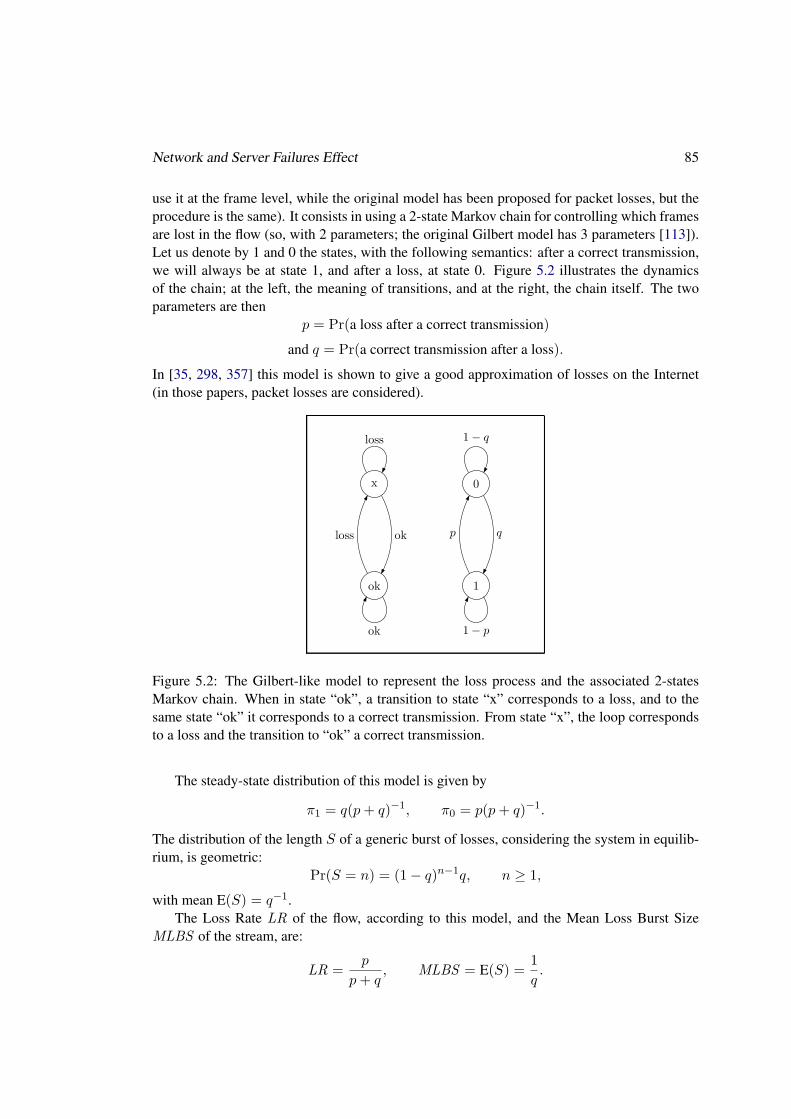
Network and Server Failures Effect 85
use it at the frame level, while the original model has been proposed for packet losses, but theprocedure is the same). It consists in using a 2-state Markov chain for controlling which framesare lost in the flow (so, with 2 parameters; the original Gilbert model has 3 parameters [113]).Let us denote by 1 and 0 the states, with the following semantics: after a correct transmission,we will always be at state 1, and after a loss, at state 0. Figure 5.2 illustrates the dynamicsof the chain; at the left, the meaning of transitions, and at the right, the chain itself. The twoparameters are then
p = Pr(a loss after a correct transmission)
and q = Pr(a correct transmission after a loss).
In [35, 298, 357] this model is shown to give a good approximation of losses on the Internet(in those papers, packet losses are considered).
ok
x
loss ok
ok
loss
1
0
p q
1− p
1− q
Figure 5.2: The Gilbert-like model to represent the loss process and the associated 2-statesMarkov chain. When in state “ok”, a transition to state “x” corresponds to a loss, and to thesame state “ok” it corresponds to a correct transmission. From state “x”, the loop correspondsto a loss and the transition to “ok” a correct transmission.
The steady-state distribution of this model is given by
π1 = q(p+ q)−1, π0 = p(p+ q)−1.
The distribution of the length S of a generic burst of losses, considering the system in equilib-rium, is geometric:
Pr(S = n) = (1− q)n−1q, n ≥ 1,
with mean E(S) = q−1.The Loss Rate LR of the flow, according to this model, and the Mean Loss Burst Size
MLBS of the stream, are:
LR =p
p+ q, MLBS = E(S) =
1q.

86 Studying the Effects of Several Parameters on the Perceived Video Quality
Reciprocally, if we have measured the Loss Rate of a stream LR (0 < LR < 1) and itsMean Loss Burst Size MLBS (MLBS ≥ 1), the (only) values of p and q leading to these LRand MLBS are
q =1
MLBS, p =
LR1− LR
1MLBS
.
We implement the Gilbert model as a module in the VLC software player, in order tocontrol the parameters, LR and MLBS , over original video sequences. It allow us to see itsquality effects in real–time, and to save the distorted video sequences.
5.2.2 Experiment Description
We applied the PSQA technique, as explained in Chapter 4. This involved choosing four MPEG-2 video sequences, of about 10 seconds duration each, with sizes between 1.5 MB and 2.8 MB).For each sequence, we generated twenty five different configurations, where each configurationis defined by a loss rate value chosen at random with an uniform distribution between 0.0 and0.2, and a mean loss burst size value chosen at random with an uniform distribution between0.0 and 4.0. For each configuration, we used a simplified Gilbert model (discussed previously)to simulate a frame drop history which was applied to the original video sequences. In this way,we obtained one hundred modified video sequences with variable quality levels. In Figure 5.3we present the final dispersion of the distorted video sequences with respect to the paramtersLR and MLBS .
1
2
3
4
5
6
7
8
9
10
0 0.02 0.04 0.06 0.08 0.1 0.12 0.14 0.16 0.18 0.2
MLB
S
LR
Test Data Dispersion
Figure 5.3: Network and Server failures Effect. Video sequences dispersion.
A group of five experts evaluated the distorted sequences and the MOS for each of thecopies was computed, following the ITU-R BT.500-11 [171] norm. See Figure 5.4 for theMOS value and the experts’ votes for each sequence. The average standard deviation of thesubjects (computed with Equation 4.2) is δ = 0.13. It means that on the average the expertsdiffered in ±13% of their assessments.

Network and Server Failures Effect 87
0
2
4
6
8
10
0 10 20 30 40 50 60 70 80 90 100
qual
ity
video sequence
Test results
usersMOS
Figure 5.4: Network and Server failures Effect. Subjective test results for building the PSQAmetric.
Next, we use the MOS value for each of the sampled points as inputs in order to approxi-mate a quality function of the two variables, LR and MLBS .
5.2.3 PSQA Simple Function
To obtain the perceptual quality as a function of the parameters that approximate smoothly theempirical test values obtained previously, we train a Random Neural Network (RNN) followingthe procedure described in Section 4.5.
In this quite simple function (because of the fact that we use only two input variables), weuse a three–layer feed–forward neural network. It consists of two neurons in the input layer,seven neurons in the hidden layer, and an output neuron. See the simple RNN topology inFigure 5.5).
To determine the number of neurons in the hidden layer we follow the procedure describedin Section 4.5.3.2 which iterate with different configurations and chooses the best one in termsof performance. To measure the performance we use the Mean Square Error (average squareddifference between the values of the function and the MOS given by real human observers). Weuse eighty-five distorted video sequences to train the RNN, and the remaining sequences (fif-teen) to validate it. We obtain a global performance of MSEsimple = 0.023 for the validation se-quence set. Comparing the estimation of the standard deviation (δsimple =
√MSEsimple = 0.15)
with the average standard deviation of the subjects (δ = 0.13) we conclude that our SimpleFunction behaves as to an average human subject.
In Figure 5.6 we can see the PSQA function. For ease of reading, we extrapolated the curveto the borders, but observe that the data are accurate and used on an internal region ([1%, 20%]for LR, and [1, 10] for the MLBS )1. We can see that quality is monotone in the two variables,
1The perceptual quality decreases quickly with high loss rate values (LR > 20% ), therefore it is possible to

88 Studying the Effects of Several Parameters on the Perceived Video Quality
Figure 5.5: Simple RNN Topology.
0
0.2
0.4
0.6
0.8
12
4
6
8
10
1
2
3
4
5
6
7
8
9
10
MLBS
PSQA
LR
Q
Figure 5.6: The PSQA Simple Function (mapping LR and MLBS into perceived quality) aftertrained and validated.
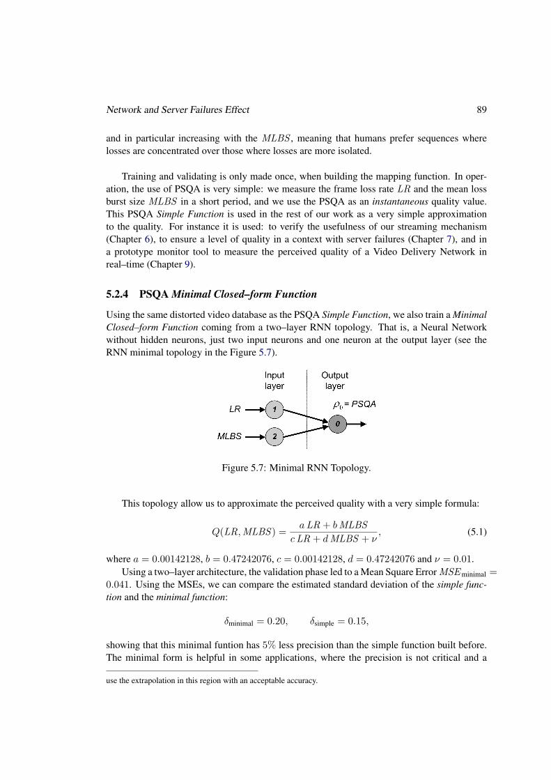
Network and Server Failures Effect 89
and in particular increasing with the MLBS , meaning that humans prefer sequences wherelosses are concentrated over those where losses are more isolated.
Training and validating is only made once, when building the mapping function. In oper-ation, the use of PSQA is very simple: we measure the frame loss rate LR and the mean lossburst size MLBS in a short period, and we use the PSQA as an instantaneous quality value.This PSQA Simple Function is used in the rest of our work as a very simple approximationto the quality. For instance it is used: to verify the usefulness of our streaming mechanism(Chapter 6), to ensure a level of quality in a context with server failures (Chapter 7), and ina prototype monitor tool to measure the perceived quality of a Video Delivery Network inreal–time (Chapter 9).
5.2.4 PSQA Minimal Closed–form Function
Using the same distorted video database as the PSQA Simple Function, we also train a MinimalClosed–form Function coming from a two–layer RNN topology. That is, a Neural Networkwithout hidden neurons, just two input neurons and one neuron at the output layer (see theRNN minimal topology in the Figure 5.7).
Figure 5.7: Minimal RNN Topology.
This topology allow us to approximate the perceived quality with a very simple formula:
Q(LR,MLBS ) =aLR + bMLBS
cLR + dMLBS + ν, (5.1)
where a = 0.00142128, b = 0.47242076, c = 0.00142128, d = 0.47242076 and ν = 0.01.Using a two–layer architecture, the validation phase led to a Mean Square Error MSEminimal =
0.041. Using the MSEs, we can compare the estimated standard deviation of the simple func-tion and the minimal function:
δminimal = 0.20, δsimple = 0.15,
showing that this minimal funtion has 5% less precision than the simple function built before.The minimal form is helpful in some applications, where the precision is not critical and a
use the extrapolation in this region with an acceptable accuracy.
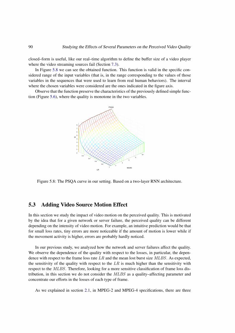
90 Studying the Effects of Several Parameters on the Perceived Video Quality
closed–form is useful, like our real–time algorithm to define the buffer size of a video playerwhere the video streaming sources fail (Section 7.3).
In Figure 5.8 we can see the obtained function. This function is valid in the specific con-sidered range of the input variables (that is, in the range corresponding to the values of thosevariables in the sequences that were used to learn from real human behaviors). The intervalwhere the chosen variables were considered are the ones indicated in the figure axis.
Observe that the function preserve the characteristics of the previously defined simple func-tion (Figure 5.6), where the quality is monotone in the two variables.
0
0.2
0.4
0.6
0.8
12
4
6
8
10
1
2
3
4
5
6
7
8
MLBS
PSQA
LR
Q
Figure 5.8: The PSQA curve in our setting. Based on a two-layer RNN architecture.
5.3 Adding Video Source Motion Effect
In this section we study the impact of video motion on the perceived quality. This is motivatedby the idea that for a given network or server failure, the perceived quality can be differentdepending on the intensity of video motion. For example, an intuitive prediction would be thatfor small loss rates, tiny errors are more noticeable if the amount of motion is lower while ifthe movement activity is higher, errors are probably hardly noticed.
In our previous study, we analyzed how the network and server failures affect the quality.We observe the dependence of the quality with respect to the losses, in particular, the depen-dence with respect to the frame loss rate LR and the mean lost burst size MLBS . As expected,the sensitivity of the quality with respect to the LR is much higher than the sensitivity withrespect to the MLBS . Therefore, looking for a more sensitive classification of frame loss dis-tribution, in this section we do not consider the MLBS as a quality–affecting parameter andconcentrate our efforts in the losses of each type of frame.
As we explained in section 2.1, in MPEG-2 and MPEG-4 specifications, there are three

Adding Video Source Motion Effect 91
main frame types: the Intra frames (I), the Predicted frames (P), and the Bidirectional or In-terpolated frames (B). In both specifications, the idea behind compression is the same: thenumerous temporal redundancies between frames are exploited using the P and B frames, bymeans of using motion estimation and compensation.
Besides the frequency and mean size of each kind of frame, they also differ in how theloss of each of them influences the quality. As there is inter-dependency among them for per-forming the codification process, if the most important frame is lost the codification is stronglyaffected, diminishing the perceived quality.
In this section we study the impact on the quality of the combination of the loss rates perframe type, instead of previous global frame loss distribution. Also this loss process classifi-cation fits better with our main objective of studying the video source motion effect, because Pand B frames are basically an abstraction of the video motion.
5.3.1 Quality-affecting parameters
As said before, the video motion is represented in MPEG standards mainly in P and B frames,using motion vector descriptions. Transmitting more information in P and B frames impliesmore motion vector descriptions; and therefore, more motion activity. Following this idea, westudy and compare the effect of bytes lost of each kind of frame, instead of just its frequencyof loss. We analyze the effect of the following distribution parameters on the quality:
I-Frames Loss Rate. In this case, ten seconds videos are considered, so there is basicallyonly one GOP in each sequence, which implies that this parameter can be only 1 or 0.We denoted it by LRI .
P-Frames Loss Rate. This parameter measures the P-Frames bytes lost in one GOP overthe total amount of P-Frames bytes in the GOP. We tested another option consisting inmeasuring the percentage of P-frames lost per GOP. It is denoted by LRP .
B-Frames Loss Rate. The same as for P-Frames, but in this case for B-Frames. It is denotedby LRB .
These first three parameters are loss rates, coming from network or server failures.
With regard to the source parameters, we study the effect of two raw (and simple) repre-sentations of the video motion activity:
Average GOP Size. The encoder decides when I-Frames are introduced, depending on thevideo characteristics, so this parameter reflects if the video sequence has many suddenchanges or not. We denoted it by GOP. Usually there is a GOP per each video scene, sothe average GOP size is close related to the number of scenes in the video, which are themost important motion activity in a video.
P-Frames Weight per GOP. This parameter indicates the weight in bytes of P-Frames ineach GOP, which is also something that depends on the video characteristics used by the

92 Studying the Effects of Several Parameters on the Perceived Video Quality
encoder to decide how to encode the sequence. The P-Frame weight per GOP represents,in a very simple way, the motion inside a scene.
Next we will show the impact of these new input parameters into the perceived quality. Ap-pendix A compares our simplest video motion parameters indicators with more sophisticatedmotion activity measures, like the MPEG-7 [51] motion descriptor and other related works.The main conclusion of this appendix is that a very low improves on the quality assessmentprecision is obtained using complex metrics to compute the motion activity. In our context, areal–time application, they not justify the computational effort.
5.3.2 Experiment Description
To apply our PSQA technique, we used fifty MPEG-4 video sequences2, of about 10 secondseach, with sizes between 238 KB and 2.78 MB. These video sequences were chosen in orderto cover the source parameter ranges. The dispersion of the source parameters is shown inFigure 5.9(a).
With this set of fifty videos, a set of 204 distorted sequences was generated, for coveringthe different possibles values for all the parameters related with the loss process (LRI , LRP
and LRB). We used a simplified Gilbert model (discussed previously) to simulate the framedrop history which was applied to the original video sequences. Half of the distorted videosincluded the I frames (LRI = 0), and the other half didn’t (LRI = 1). This is because in aMPEG-4 video sequence of 10 seconds, there are at most only one I frame. With respect toLRP and LRB , the final dispersion is shown in Figure 5.9(b).
0.5
0.55
0.6
0.65
0.7
0.75
0.8
0.85
0.9
0 50 100 150 200 250 300 350 400
P-F
ram
es W
eigh
t per
GO
P.
Average GOP size
Test Data Dispersion
(a) Average GOP Size and P-Frames Weight per GOP.
0
0.05
0.1
0.15
0.2
0.25
0 0.05 0.1 0.15 0.2 0.25 0.3
B-F
ram
es L
oss
Rat
e
P-Frames Loss Rate
Test Data Dispersion
(b) LRP and LRB .
Figure 5.9: Motion Effect. Video sequences dispersion.
Then, a group of ten experts evaluated the 204 distorted video sequences and the MOS foreach of the sequences was computed, following the Section 4.4 (Single Stimulus (SS) subjec-tive test of the ITU-R BT.500-11 recommendation [171]). See Figure 5.4 for the MOS valueand the experts’ votes for each sequence.
2We used the Xvid [354] codec implementation of MPEG-4.
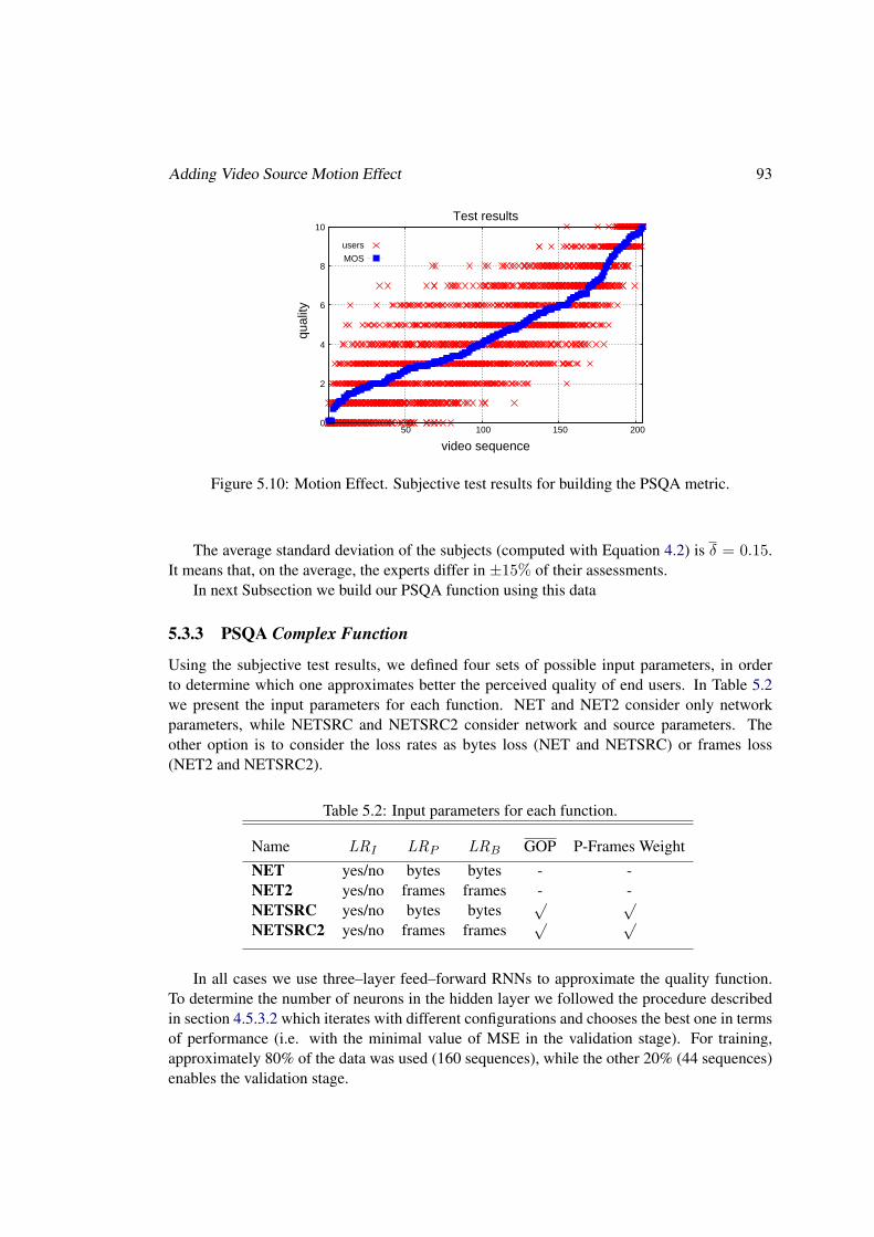
Adding Video Source Motion Effect 93
0
2
4
6
8
10
50 100 150 200
qual
ity
video sequence
Test results
users
MOS
Figure 5.10: Motion Effect. Subjective test results for building the PSQA metric.
The average standard deviation of the subjects (computed with Equation 4.2) is δ = 0.15.It means that, on the average, the experts differ in ±15% of their assessments.
In next Subsection we build our PSQA function using this data
5.3.3 PSQA Complex Function
Using the subjective test results, we defined four sets of possible input parameters, in orderto determine which one approximates better the perceived quality of end users. In Table 5.2we present the input parameters for each function. NET and NET2 consider only networkparameters, while NETSRC and NETSRC2 consider network and source parameters. Theother option is to consider the loss rates as bytes loss (NET and NETSRC) or frames loss(NET2 and NETSRC2).
Table 5.2: Input parameters for each function.
Name LRI LRP LRB GOP P-Frames WeightNET yes/no bytes bytes - -NET2 yes/no frames frames - -NETSRC yes/no bytes bytes
√ √NETSRC2 yes/no frames frames
√ √
In all cases we use three–layer feed–forward RNNs to approximate the quality function.To determine the number of neurons in the hidden layer we followed the procedure describedin section 4.5.3.2 which iterates with different configurations and chooses the best one in termsof performance (i.e. with the minimal value of MSE in the validation stage). For training,approximately 80% of the data was used (160 sequences), while the other 20% (44 sequences)enables the validation stage.

94 Studying the Effects of Several Parameters on the Perceived Video Quality
The best results are resumed in Table 5.3. Tests showed no significant differences betweenthe cases which consider bytes loss and the ones with frames loss, which can be seen comparingNET and NET2 and the same between NETSRC and NETSRC2. A small improvement is seenin the case of NETSRC2, considering frames loss, while a more important improvement is seencomparing the systems which only use network parameters with the ones which add sourceparameters.
Table 5.3: Best RNN for each input parameter set.
Name Hidden MSEneurons validation
NET 2 0.0296717NET2 6 0.0288654NETSRC 3 0.0281829NETSRC2 3 0.0254898
Figure 5.11: Complex NETSRC2 RNN Topology.
We choose the best performance RNN, NETSRC2, as our Complex Function. See the com-plex RNN topology in Figure 5.11. We obtain a global performance of MSEcomplex = 0.025for the validation sequence set. Comparing the estimation of the standard deviation (δcomplex =√
MSEcomplex = 0.16) with the average standard deviation of the subjects (δ = 0.15) we con-clude that our Complex Function behaves very similar to an average human subject.
With our Complex Function, the loss rate effect of each frame type is illustrated in Fig-ures 5.12, 5.13(b) and 5.13(a). The figures show the perceived quality as a function of two

Adding Video Source Motion Effect 95
parameters, the other three parameters (hidden in the figures) are fixed with the following val-ues: there are no hidden losses, the average value is used for the source parameters (GOP = 174and P-Frames Weight = 0.7007).
In Figure 5.12, quality degrades quickly with an increment in the loss rate of frames I andP. For example, for LRP ≥ 10% the quality is less than 6 (between good-fair) and the impactof P-frames’ losses is a bit higher than for I-frames. Figures 5.13(b) and 5.13(a) show that thequality degrades slowly with an increment in the loss rate of B-frames, as expected.
0
0.2
0.4
0.6
0.8
1
0
0.2
0.4
0.6
0.8
1
2
3
4
5
6
7
8
9
10
Loss rate I
Perceptual quality
Loss rate P
Q
Figure 5.12: The quality degrades quickly with an increment in the loss rates of frames I and P.
0
0.2
0.4
0.6
0.8
1
0
0.2
0.4
0.6
0.8
1
3
4
5
6
7
8
9
10
Loss rate I
Perceptual quality
Loss rate B
Q
(a) LRB vs. LRI .
0
0.2
0.4
0.6
0.8
1
0
0.2
0.4
0.6
0.8
1
2
3
4
5
6
7
8
9
10
Loss rate P
Perceptual quality
Loss rate B
Q
(b) LRB vs. LRP .
Figure 5.13: The quality degrades slowly with an increment in the loss rate of frames B.

96 Studying the Effects of Several Parameters on the Perceived Video Quality
The source parameters do not directly degrade the quality, but they have an impact on howlosses affect users’ perception. To observe the effect of source parameters into quality, we showtheir impact with respect to each kind of frame lost independently. In Figures 5.14(a), 5.14(b)and 5.14(c) we show the influence of the P-frames weight per GOP. As we expect, with higherratios of P-frames weight, there is less impact of I-frames and B-frames losses into the quality.
0
0.2
0.4
0.6
0.8
1 0
0.2
0.4
0.6
0.8
1
1
2
3
4
5
6
7
8
9
10
Loss rate I
Perceptual quality
P−Frames Weight
Q
(a) P-Frames Weight vs LRI .
0
0.2
0.4
0.6
0.8
1 0
0.2
0.4
0.6
0.8
1
1
2
3
4
5
6
7
8
9
10
Loss rate P
Perceptual quality
P−Frames Weight
Q
(b) P-Frames Weight vs LRP .
0
0.2
0.4
0.6
0.8
1 0
0.2
0.4
0.6
0.8
1
4
5
6
7
8
9
10
Loss rate B
Perceptual quality
P−Frames Weight
Q(c) P-Frames Weight vs LRB .
Figure 5.14: P-Frames Weight influences into the quality to different kind of frame losses.
In Figures 5.15(a), 5.15(b) and 5.15(c) we show the influence of the average GOP size. Wesee that there is no observable influence of GOP size into the quality in a scenario of losses.
0
100
200
300
400 0
0.2
0.4
0.6
0.8
1
5
6
7
8
9
10
Loss rate I
Perceptual quality
GOP size
Q
(a) GOP size vs LRI .
0
100
200
300
400 0
0.2
0.4
0.6
0.8
1
2
3
4
5
6
7
8
9
10
Loss rate P
Perceptual quality
GOP size
Q
(b) GOP size vs LRP .
0
100
200
300
400 0
0.2
0.4
0.6
0.8
1
6.5
7
7.5
8
8.5
9
9.5
10
Loss rate B
Perceptual quality
GOP size
Q
(c) GOP size vs LRB .
Figure 5.15: Average GOP size influences into the quality to different kind of frame losses.
The Complex Function is used in the rest of our work. In section 7.2, we find an optimalstreaming method, from the user point of view (evaluating the perceived quality with this func-tion), in a context of server failures. We also use it in our P2P prototype, GOL!P2P, for robustdelivery of high quality live video (see chapter 10). In this prototype we measure the perceivedquality by each user in real–time, and take control actions with this information.
5.4 Summary and Conclusions
In this chapter we studied the effects of network and source parameters on the perceived videoquality evaluated using the PSQA methodology (explained in Chapter 4). We applied the PSQA

Summary and Conclusions 97
technique in two scenarios. First, we analyzed the network and server failures impact on qual-ity by means of the study of frame lost effect. Second, we improved the measure accuracyconsidering the influence of video source’ motion in quality.
This study extends and generalizes previous works on PSQA, in particular for video qualityassessment, evaluating the effect at the frame level (instead of packet level studied previously).The mapping functions (from quality–affecting parameters into perceived quality) obtained inthis chapter will be used in the rest of this work for network design purposes and for perfor-mance evaluation.

98 Studying the Effects of Several Parameters on the Perceived Video Quality

Part III
PEER-TO-PEER
99


Chapter 6
Multi-Source Streaming Technique
In this chapter we address the problem of designing a content distribution technique for real-time video delivery through a P2P system on the Internet. The main advantage of using theP2P approach is to exploit the available bandwidth unused by the set of machines connectedto the network. The main difficulty is that these machines are typically highly dynamic withrespect to the network, they continuously enter and leave it. To deal with this problem, weexplore a multi-source approach where the stream is decomposed into several redundant flowssent by different peers to each client. Using the PSQA technology (detailed in Chapter 4)for evaluating automatically and accurately the perceived quality at the client side, this chapterfocuses on the consequences that the way the stream is decomposed has on the resulting quality.
Our approach allows thus to do the design by addressing the ultimate target, the perceivedquality (or Quality of Experience), instead of the standard but indirect metrics such as loss rates,delays, reliability, etc. The main contribution of this chapter is to provide a global methodologythat can be used to design such a system, illustrated by looking at three extreme cases. Anotherimportant feature of our technique is that it results in a very low signaling cost (overhead), incontrast with Bittorrent-like approaches.
The chapter is organized as follows. Section 6.1 introduces multi-source streaming tech-niques. In Section 6.2 we develop models to estimate the streaming performance, in a envi-ronment with server nodes failures. The conclusions of the chapter are summarized in Sec-tion 6.3. This chapter has been partially presented at the IEEE Global TelecommunicationsConference (GLOBECOM’07)[282] and Beijing-Hong Kong International Doctoral Forum -Web, Network, and Media Computing (BJ-HK Phd Forum’07)[275] (listed at the Introductionas [globecom07] and [bj-hk07]).
6.1 Introduction to multi-source streaming
In this chapter, we are interested in some aspects related to the use of a P2P architecture todistribute live video. Using a P2P infrastructure for video distribution looks like a good ideadue to the high requirements in terms of bandwidth of these applications. The main problem is
101

102 Multi-Source Streaming Technique
how to provide good quality levels in a context where this quality depends on other clients thatare delivering the stream, and given the fact that users connect and disconnect very frequently.The main idea that has been considered to deal with these problems is to build the systemsusing some redundancy in the signals. In this thesis we explore one of ways to reach thisobjective: multi-source streaming. This means that the live video stream is received by theclient from flows sent by many sources simultaneously. This needs some degree of intelligenceon the senders that build a set of sub-streams from an original one, allowing to re-compose thestream to be played with the different received components, and some degree of intelligence onthe client side, for performing this last task, and perhaps for building a satisfactory stream evenwhen some of those components are missing. This approach allows for a large flexibility of thesystem, modulated by the dynamics of the network. In particular, it is in principle possible toincrease the number of sources and/or the amount of redundant information sent through thenetwork; this flexibility can be used as a tool to deal with the problem of nodes leaving thenetwork and causing partial signal losses to some clients. We will say that a node fails to referto the fact that it leaves the network.
The system’s flexibility must be carefully tuned in order to get a satisfactory quality levelat a minimal cost. The usual approach is to focus on a well chosen metric, that we know playsan important role in quality, such as the loss rate of packets, or of frames. In this work weinstead address the problem of measuring perceived quality by means of the PSQA technology(see Part II). PSQA is a general procedure that allows the automatic measure of the perceivedquality, accurately and in real-time.
Summarizing, in order to face the high dynamics of a P2P live video distribution network,we explore a multi-path approach where (i) the stream is decomposed in some way into severalflows, (ii) each client receives several flows following different paths and sent from differentother clients, (iii) the client is able to reconstruct the stream from the whole set of received flowsand possibly from part of them; moreover, (iv) the system measures automatically the perceivedquality at the client continuously, and takes its decisions (basically, periodically rebuilding thearchitecture of the network) using these values.
6.1.1 Simple extreme multi-source methods: single, copied and splitted flows
The main architecture we are considering is the following one. Some server producing a livevideo stream splits this stream into K flows, with some amount of redundancy in them (thatis, together they can transport “more information” than contained in the original video signal),and it sends each of these flows to a specific set of clients. The clients in turn send the receivedflows to other nodes. The architecture must ensure that each client receives the different flowsfrom different nodes. So, from the client’s point of view, we have a multi-source deliveringsystem.
Please note that, for a simplified notation, and with the idea of the client point of view, inour explanation we have one client and a set of K servers, where actually the servers are otherpeers of the P2P network, and also the client can serve to other peers.
The simplest situation is when there is a single server node which sends all the streaminginformation to the clients (see Figure 6.1). Let us consider instead the case where a set of
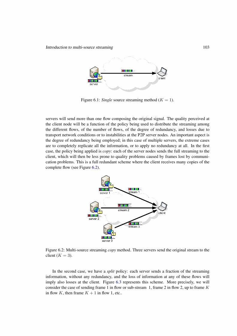
Introduction to multi-source streaming 103
Figure 6.1: Single source streaming method (K = 1).
servers will send more than one flow composing the original signal. The quality perceived atthe client node will be a function of the policy being used to distribute the streaming amongthe different flows, of the number of flows, of the degree of redundancy, and losses due totransport network conditions or to instabilities at the P2P server nodes. An important aspect isthe degree of redundancy being employed; in this case of multiple servers, the extreme casesare to completely replicate all the information, or to apply no redundancy at all. In the firstcase, the policy being applied is copy: each of the server nodes sends the full streaming to theclient, which will then be less prone to quality problems caused by frames lost by communi-cation problems. This is a full redundant scheme where the client receives many copies of thecomplete flow (see Figure 6.2).
Figure 6.2: Multi-source streaming copy method. Three servers send the original stream to theclient (K = 3).
In the second case, we have a split policy: each server sends a fraction of the streaminginformation, without any redundancy, and the loss of information at any of these flows willimply also losses at the client. Figure 6.3 represents this scheme. More precisely, we willconsider the case of sending frame 1 in flow or sub-stream 1, frame 2 in flow 2, up to frame Kin flow K, then frame K + 1 in flow 1, etc..

104 Multi-Source Streaming Technique
Figure 6.3: Multi-source streaming split method. Three servers send three different and noredundant sub-streams to the client (K = 3).
A situation between these two extreme policies is to split the stream into K redundant sub-streams, with the necessary redundancy to avoid losses during a single server disconnection.This means that each frame is sent exactly twice (by two different servers to a given client).Figure 6.4 represents this scheme.
Figure 6.4: Multi-source streaming redundant split method. Three servers send three differentredundant sub-streams to the client (K = 3).
Obviously, we can expect that in a scenario subject to failures, with more redundancy betterquality will be achieved. The cost of this improvement is a larger bandwidth consumption. Ifthe bandwidth of the original stream is B, then the bandwidth of the copy method is KB, Bfor the simple split method, and 2B for the redundant split method.

Introduction to multi-source streaming 105
Although in this chapter we concentrate on these extreme policies (either zero redundancy,full replication of the information sent by each server, or redundancy to avoid losses duringone server fault), it is clear that the degree of redundancy admits many other possibilities in-between. In next chapter we present an optimal streaming technique (between these simplecases), which also considers the heterogeneity of the peers dynamics.
6.1.2 Related multi-source strategies
Previous studies (see [18]) show that in 30-80% of the cases for a given transmission thereis at least an end-to-end path better (from the quality perspective) than the one chosen byusual protocols. This is the main idea behind the multi-path and path diversity studies. In theparticular case of video flows, it is easier to recover from isolated losses than from consecutiveones [17]. The basic difference between the multi-path and multi-source concepts is that inthe former case we consider a single source sending data to the destination following differentpaths. The main difficulty here is the routing aspects: we must specify and control which pathmust be followed by which packet in the flow. The multi-source approach implies that thereare multiple and independent sources for the signal, and that some general scheme allows thereceiver to get the stream from a set of servers. Since they are different, the path that the packetswill follow would be a priori different, without any need of acting on the routing processes. Ofcourse, in practice, the different paths could share some nodes, which are good candidates tobecome bottlenecks of the communication system. Detecting such cases is an active researcharea [291].
Focusing on P2P applications, observe first that many P2P data sharing and distributionsystems implicitly assume that a sending peer is capable of supporting one or more receivingpeers. It can be complicated to implement this in practice, especially for video streaming.
The same proposals suggest to implement the multi-source streaming at the video encodinglevel, using the Multiple Description Coding (MDC) [16, 118, 191, 204, 304]. MDC is a videocoding technique, which generates an arbitrary number of sub-streams (called descriptions, inthis context) from one single stream. Each sub-stream can be decoded independently fromthe others; however, the quality improves when more descriptions are decoded in parallel. InMPEG-2 and MPEG-4, it is possible to encode a video in layers. Similar to MDC, layeredcoding techniques generate an arbitrary number of layers, and the quality improves when morelayers are decoded. But here, there are a base layer and a series of hierarchical enhancementlayers. In order to decode a layer is necessary to decode the layer immediate before (they arenot independent of each other). MDC and layered coding are developed to allow a finer controlof the streaming and to provide error resilience to media streams. Both have high complexity,with less efficient compression. Therefore, they are not widely deployed, and there are noopen-source implementations.
Other works propose to implement the multi-source streaming at the transport level, forinstance using Network Coding [6, 55, 56]. Network Coding is a method based on informationand coding theories, that allows to mix the data at intermediate network nodes, while the re-ceiver extracts form these data the original message. It attempts to maximize the informationflow in a network. Network Coding is not necessarily suitable for P2P networks; the dynamicsof the overlay topology, and the time needed by peers to decode data encoded with this proce-
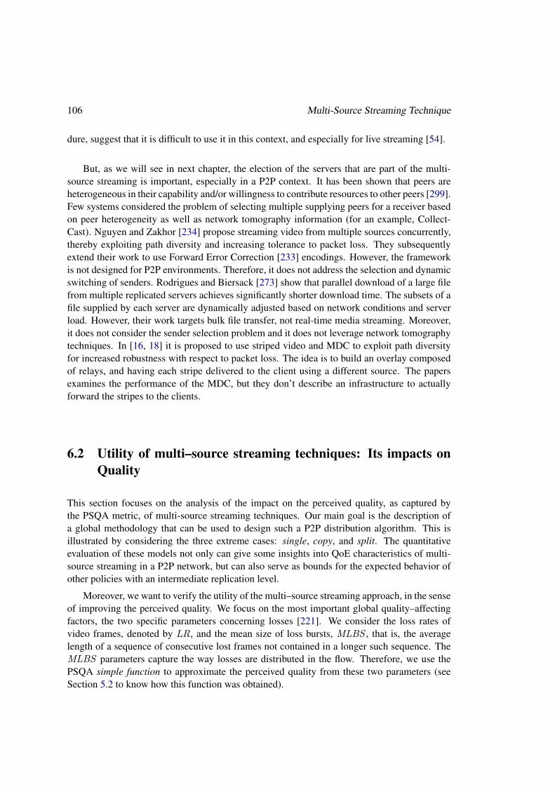
106 Multi-Source Streaming Technique
dure, suggest that it is difficult to use it in this context, and especially for live streaming [54].
But, as we will see in next chapter, the election of the servers that are part of the multi-source streaming is important, especially in a P2P context. It has been shown that peers areheterogeneous in their capability and/or willingness to contribute resources to other peers [299].Few systems considered the problem of selecting multiple supplying peers for a receiver basedon peer heterogeneity as well as network tomography information (for an example, Collect-Cast). Nguyen and Zakhor [234] propose streaming video from multiple sources concurrently,thereby exploiting path diversity and increasing tolerance to packet loss. They subsequentlyextend their work to use Forward Error Correction [233] encodings. However, the frameworkis not designed for P2P environments. Therefore, it does not address the selection and dynamicswitching of senders. Rodrigues and Biersack [273] show that parallel download of a large filefrom multiple replicated servers achieves significantly shorter download time. The subsets of afile supplied by each server are dynamically adjusted based on network conditions and serverload. However, their work targets bulk file transfer, not real-time media streaming. Moreover,it does not consider the sender selection problem and it does not leverage network tomographytechniques. In [16, 18] it is proposed to use striped video and MDC to exploit path diversityfor increased robustness with respect to packet loss. The idea is to build an overlay composedof relays, and having each stripe delivered to the client using a different source. The papersexamines the performance of the MDC, but they don’t describe an infrastructure to actuallyforward the stripes to the clients.
6.2 Utility of multi–source streaming techniques: Its impacts onQuality
This section focuses on the analysis of the impact on the perceived quality, as captured bythe PSQA metric, of multi-source streaming techniques. Our main goal is the description ofa global methodology that can be used to design such a P2P distribution algorithm. This isillustrated by considering the three extreme cases: single, copy, and split. The quantitativeevaluation of these models not only can give some insights into QoE characteristics of multi-source streaming in a P2P network, but can also serve as bounds for the expected behavior ofother policies with an intermediate replication level.
Moreover, we want to verify the utility of the multi–source streaming approach, in the senseof improving the perceived quality. We focus on the most important global quality–affectingfactors, the two specific parameters concerning losses [221]. We consider the loss rates ofvideo frames, denoted by LR, and the mean size of loss bursts, MLBS , that is, the averagelength of a sequence of consecutive lost frames not contained in a longer such sequence. TheMLBS parameters capture the way losses are distributed in the flow. Therefore, we use thePSQA simple function to approximate the perceived quality from these two parameters (seeSection 5.2 to know how this function was obtained).

Utility of multi–source streaming techniques: Its impacts on Quality 107
6.2.1 Multi-source Streaming Models
We develop here stochastic (Markovian) models for the frame loss process in multi-sourcestreaming, in the three considered cases.
We start from the single source case, using one of the simplest models considered in theliterature, which nevertheless can take into account the two chosen parameters of the loss pro-cess, LR and MLBS . We do not differentiate among losses due to the server node itself andlosses due to the underlying Internet connection between server and client; we just apply adescriptive model, whose parameters can be completely characterized by the observed valuesof the above mentioned LR and MLBS parameters1.
6.2.1.1 Streaming from a single source
To model the loss process on an end-to-end communication we used the so-called simplifiedGilbert model, presented in Section 5.2.1.1. It consists of using a 2-state Markov chain forcontrolling which frames are lost in the flow (see Figure 5.2 for a illustration of the chaindynamics). It has two parameters:
p = Pr(a loss after a correct transmission)
andq = Pr(a correct transmission after a loss).
Summarizing, the steady-state distribution of this model is given by π1 = q(p + q)−1,π0 = p(p + q)−1. The distribution of the length S of a generic burst of losses, consideringthe system in equilibrium, is geometric: Pr(S = n) = (1 − q)n−1q, n ≥ 1, with meanE(S) = q−1. Finally, the Loss Rate LR of the flow, according to this model, and the MeanLoss Burst Size MLBS of the stream, are
LR =p
p+ q, MLBS = E(S) =
1q.
6.2.1.2 Sending K copies of the stream
Assume there are K copies of the same stream travel following independent and stochasticallyequivalent paths to the same terminal. The loss process at any of the K streams is representedby the model previously described, with parameters p and q. It is clear that the receiver willobserve the loss of a frame if all the copies of the frames are lost. If LRcopy
K denotes this globalLoss Rate, we then have
LRcopyK =
(p
p+ q
)K= LRK .
If SK denotes the size of a generic burst of losses, we have
Pr(SK = n) =[(1− q)K]n−1 [
1− (1− q)K] ,1In a P2P network, we expect that the losses due to server disconnections dominate those due to the best-effort
Internet. We keep the two possibilities for generality reasons.

108 Multi-Source Streaming Technique
giving a global Mean Loss Burst Size MLBS copyK = E(SK) as follows:
MLBS copyK =
11− (1− q)K =
11− (1−MLBS−1)K
.
6.2.1.3 Complete split of the stream into K ≥ 2 sub-streams
In the other extreme case considered in this section, we have K sub-streams transporting eacha 1/K fraction of the frames in the following way: frame 1 goes through sub-stream 1, frame2 through sub-stream 2, until frame K going through sub-stream K, then frame K+ 1 throughsub-stream 1, etc. In general, frame n is sent by sub-stream ((n− 1) mod K) + 1.
Again, the loss processes at any of the K streams are stochastically equivalent, and arerepresented by the previous model, with parameters p and q. We obviously have here, for theLoss Rate of this scheme, the same value as for the single source case:
LRsplitK = LR = p(p+ q)−1.
The evaluation of the Mean Loss Burst Size is more involved. The probability Pr(SK = 1)is the probability that after a loss (which follows a correct transmission), next packet is notlost. For Pr(SK = 2), observe that a burst has size 2 if after the first loss (following a correcttransmission), we have a loss and then a correct transmission. And so on.
Consider first the case ofK = 2. The probability Pr(S2 = 1) is 1−p, because sinceK = 2and the case of interest (S2 = 1) corresponds to the sequence ‘1 0 1’, the state of the simplifiedGilbert model in the sub-stream corresponding to the last ‘1’ is ‘1’ (the state after a correcttransmission); the associated conditional probability is 1 − p. So, Pr(S2 = 1) = 1 − p. ForS2 = 2, we have the pattern ‘1 0 0 1’ and we want to evaluate the probability of observing thesuffix ‘0 1’ knowing that the previous pattern (the prefix) is ‘1 0’. We have Pr(S2 = 2) = pq.For size 3, we obtain Pr(S2 = 3) = p(1− q)q. Following the same reasoning, we have
Pr(S2 = n) = p(1− q)n−2q, n ≥ 2.
From this expression and after some algebra, we get
E(S2) = 1− p+∑n≥2
np(1− q)n−2q = · · · = 1 +p
q.
Let us illustrate the evaluation in the case of K = 4. The general case is done the sameway. The probability Pr(S4 = 1) is the probability that after a loss (which follows a correcttransmission), next packet is not lost. The probability of this correct transmission depends onthe state of the corresponding sub-stream: if it is ‘1’, the value is 1− p; if it is ‘0’, the value isq. Using the steady-state distribution of the simplified Gilbert model, we have
Pr(S4 = 1) = π1(1− p) + π0q = π1
(=
q
p+ q
).
For Pr(S4 = 2), we need the probability of a loss and then a correct transmission after a firstloss that follows a correct transmission. The last event (the correct transmission closing the
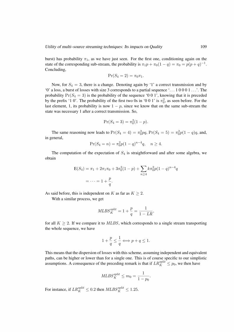
Utility of multi–source streaming techniques: Its impacts on Quality 109
burst) has probability π1, as we have just seen. For the first one, conditioning again on thestate of the corresponding sub-stream, the probability is π1p+ π0(1− q) = π0 = p(p+ q)−1.Concluding,
Pr(S4 = 2) = π0π1.
Now, for S4 = 3, there is a change. Denoting again by ‘1’ a correct transmission and by‘0’ a loss, a burst of losses with size 3 corresponds to a partial sequence ‘. . . 1 0 0 0 1 . . .’. Theprobability Pr(S4 = 3) is the probability of the sequence ‘0 0 1’, knowing that it is precededby the prefix ‘1 0’. The probability of the first two 0s in ‘0 0 1’ is π2
0 , as seen before. For thelast element, 1, its probability is now 1 − p, since we know that on the same sub-stream thestate was necessary 1 after a correct transmission. So,
Pr(S4 = 3) = π20(1− p).
The same reasoning now leads to Pr(S4 = 4) = π20pq, Pr(S4 = 5) = π2
0p(1 − q)q, and,in general,
Pr(S4 = n) = π20p(1− q)n−4q, n ≥ 4.
The computation of the expectation of S4 is straightforward and after some algebra, weobtain
E(S4) = π1 + 2π1π0 + 3π20(1− p) +
∑n≥4
kπ20p(1− q)n−4q
= · · · = 1 +p
q.
As said before, this is independent on K as far as K ≥ 2.With a similar process, we get
MLBS splitK = 1 +
p
q=
11− LR
,
for all K ≥ 2. If we compare it to MLBS , which corresponds to a single stream transportingthe whole sequence, we have
1 +p
q≤ 1q⇐⇒ p+ q ≤ 1.
This means that the dispersion of losses with this scheme, assuming independent and equivalentpaths, can be higher or lower than for a single one. This is of course specific to our simplisticassumptions. A consequence of the preceding remark is that if LRsplit
K ≤ p0, we then have
MLBS splitK ≤ m0 =
11− p0
.
For instance, if LRsplitK ≤ 0.2 then MLBS split
K ≤ 1.25.

110 Multi-Source Streaming Technique
6.2.2 Evaluating and first results
Now we can study how the frame loss rate and frame mean loss burst size parameters affect thequality (as measured by the PSQA technique) for the single server and multiple server (copyand split) streaming policies.
We use the PSQA simple function explained in Subsection 5.2.3. With this function, wecan now compare the effect of the different streaming policies on the quality perceived at theclient node. In Figures 6.5(a), 6.5(b), and 6.5(c) we see respectively the situation for the singleserver policy, the split policy with K = 2, and the copy policy with K = 2. In the threecases we have the same frame loss process going on at the server side. The figures show theperceived quality as a function of parameter LR, for different values of MLBS . In the figures,the LR and MLBS values represent the frame loss process at the servers side. In the threecases, the perceived quality deteriorates quickly with increasing values of LR; but the qualityvalues and the shape of the curves are very different for every policy. In the single server case,the behavior is almost insensitive to the MLBS parameter; the quality depends very heavily onLR, deteriorating very quickly as this parameter grows a little bit from 0. In the split policywith two servers, the effect of LR is similar; we can observe that this policy completely cancelsout the effect of the MLBS parameter at the sources. In the copy policy, the observed qualitylevels for large LR are much higher than the corresponding ones in the other two models. Herethe effect of MLBS is more pronounced than in the previous two cases, larger MLBS valueshaving rather better quality.
In order to make it easier to compare the different policies, we show in Figures 6.6(a) and6.6(b) the quality values for the three policies as a function of LR, with MLBS = 1.0 andMLBS = 4.0 respectively. These figures show how the copy policy with two servers, whichtransmits every frame twice, benefits from this redundancy and copes much better with highvalues of LR, maintaining better quality results, for both low and high MLBS scenarios. In thecase where MLBS = 1, the single and split policy give the same results (this follows directlyfrom our analytical models). When MLBS = 4, the split policy fares worse than the singlepolicy. This comes from the fact that, in this case, the split policy results in a lower value forthe MLBS perceived by the user with respect to the MLBS at the server side, and that the MOScomputed from the experts opinions show that lower MLBS result in lower quality values (i.e.the users prefer concentrated losses, and the split policy “breaks up” some of the frame losscorrelation in the transmission process).
We can conclude that (obviously) sending the signal twice leads to a much better qualitythan only once, and that sending disjoint pieces of the stream is not always useful. A non-trivialconclusion about these results is that, from quality point of view, people prefer to concentratelosses instead of spreading them (in this range of losses). These results suggest that someintermediate multi-source streaming policy, between the extreme copy and split cases, can beuseful to improve the perceived quality. Observe that the use of PSQA allows to say not onlythat the copy method is better than the split one, but for how much, and with respect to theuser’s perception point of view.

Utility of multi–source streaming techniques: Its impacts on Quality 111
1
2
3
4
5
6
7
8
9
10
0 0.02 0.04 0.06 0.08 0.1 0.12 0.14 0.16
qual
ity
lr
Single: PSQA vs. LR
mlbs=1mlbs=2mlbs=3mlbs=4
(a) Single method.
1
2
3
4
5
6
7
8
9
10
0 0.02 0.04 0.06 0.08 0.1 0.12 0.14 0.16
qual
ity
lr
Split: PSQA vs. LR
mlbs=1mlbs=2mlbs=3mlbs=4
(b) Split method.
5.5
6
6.5
7
7.5
8
8.5
9
9.5
10
0 0.02 0.04 0.06 0.08 0.1 0.12 0.14 0.16
qual
ity
lr
Copy K=2: PSQA vs. LR
mlbs=1mlbs=2mlbs=3mlbs=4
(c) Copy method.
Figure 6.5: Multi-source streaming methods, in the loss domain. The LR and MLBS valuesrepresent the frame loss process at the servers side.

112 Multi-Source Streaming Technique
1
2
3
4
5
6
7
8
9
10
0 0.02 0.04 0.06 0.08 0.1 0.12 0.14 0.16
qual
ity
lr
Single, Split and Copy K=2: PSQA vs. lr (MLBS=1)
singlesplit
copy
(a) Without bursts, MLBS = 1.
1
2
3
4
5
6
7
8
9
10
0 0.02 0.04 0.06 0.08 0.1 0.12 0.14 0.16
qual
ity
lr
Single, Split and Copy K=2: PSQA vs. lr (MLBS=4)
singlesplit
copy
(b) With bursts, MLBS = 4.
Figure 6.6: Compare multi-source streaming methods. The LR and MLBS values representthe frame loss process at the servers side.
6.3 Summary and Conclusions
This chapter proposes some general principles for the design of a live-video P2P distributionsystem following a multi-source procedure where the video stream is decomposed into differentflows that travel independently through the network. We use the PSQA technique that allowsto measure automatically the perceived quality as seen by the final users. The chapter focuseson the impact on quality (as measured by PSQA) on three extreme cases: sending the streamfrom one node to the other (for reference purposes), sending two complete copies of the streamthrough different paths, and sending two disjoint sub-streams whose union recomposes theoriginal one.
We are able to evaluate the resulting perceived quality associated with these extreme ar-chitectures. The main conclusions are: (i) thanks to an improved version of PSQA we seethat quality increases as losses concentrate in the stream (for a fixed loss rate); (ii) sending thesignal twice obviously leads to a much better quality, even if, as expected, losses are less con-centrated in this case; (iii) sending disjoint pieces of the stream is not useful, of course underour simplifying assumptions and scenarios.
This study suggests that some intermediate point between the extreme cases we considered,with a higher redundancy or with a higher number of flows per stream, can be an interestingsolution. The chapter shows the utility of the delivery technique, It also strongly suggest tolook for more realistic models. In next chapter we present a finer analysis of different splittingcases.

Chapter 7
Optimal Quality in Multi-SourceStreaming
This chapter presents a deeper study of our proposed multi-source streaming technique. Weshow, using real data, how our technique allows to compensate efficiently the possible lossesof frames due to peers leaving a P2P system. Moreover, we can statistically ensure some levelof quality, when the dynamics in the network is specified (Section 7.1). This section has beenpartially presented at the IFIP/ACM Latin America Networking Conference (LANC’07)[283]and 4th Euro-FGI workshop on “New trends in modelling, quantitative methods and measure-ments” (Euro-FGI WP IA.7.1)[281] (listed at the Introduction as [lanc07] and [euro-fgi07]).
In Section 7.2, we improve the technique in different ways, specially considering the peers’heterogeneity, we obtain an optimal multi-source streaming technique that will be used in ourGOL!P2P prototype. This result has been developed in coolaboration with A.P. Couto da Silvaand presented at the IEEE International Conference on Communications (ICC 2008)[75] (listedat the Introduction as [icc08]).
Section 7.3 studies the multi-source approach from the receiver point of view, and definesa frame buffer policy in order to ensure a given quality level. This work has been partially pre-sented at the 8th International Workshop on Performability Modeling of Computer and Com-munication Systems (PMCCS’07)[74] (listed at the Introduction as [pmccs07]), again with thecollaboration of A.P. Couto da Silva.
7.1 Video Quality Assurance: introducing the peers behavior
In Chapter 6 we presented multi-source streaming, and we studied its impacts in the quality forsimple extreme streaming policies (Section 6.2.1). This analysis was stationary, in the sensethat it showed the average quality behavior of the policies in a long term period.
The main difficulty in the design of a P2P system for distribution real-time video, is how toprovide good quality levels in a context where this quality depends on other clients that are de-livering the stream, and given the fact that users connect and disconnect very frequently. Thissection focuses then on the analysis of the impact that the peers’ dynamics (represented by atransient model) has on the perceived quality. This is presented by considering the extreme
113

114 Optimal Quality in Multi-Source Streaming
multi-source streaming cases: copy (where the flows are just copies of the original sequence,with a very high redundancy level), split (where the sequence is split into simple disjoint sub-streams, without redundancy at all), and redundant split (where the sequence is split into re-dundant sub-streams, when is possible to reconstruct completely the stream with only oneserver failure). See Section 6.1 for details on these policies. We do some experiments in orderto explore the consequences of these architecture choices on the quality level, extending thepreliminary results presented in Section 6.2.1.
To evaluate the impact of this approach on quality, we use the PSQA simple function of Sec-tion 5.2, which maps the loss rates of video frames, LR, and the mean lost burst size, MLBS ,into the perceived quality. This simple function is accurate enough to model the impact of thepeers’ behavior, illustrating with real data how the methods allow to compensate efficiently thepossible losses of frames due to peers leaving the system.
In Subsection 7.1.1 we present a P2P network for live multi-source streaming, and a tran-sient model of the nodes disconnection from the client’s perspective. Subsection 7.1.2 developsmodels to estimate the streaming performance, in a environment with server nodes fails, neededto the construction of the PSQA measuring module. These models calibrate the multi-sourcestreaming on the basis of the perceptual quality. In Subsection 7.1.3 some experimental resultsare introduced.
7.1.1 P2P Network and Dynamics Model
Multi-source streaming techniques allow for a large flexibility of the system, modulated by thedynamics of the clients. In particular, it is possible to increase the number of sources and/orthe amount of redundant information sent through the network (the three cases discussed havedifferent redundant information degree and can be potentially used with any amount of servers).
To decide which peer will serve which other nodes, some degree of intelligence and knowl-edge about the peers and the network state is needed. An important research effort is beingdone in the community on this hot topic (which will be presented in Chapter 8). The differentproposals are based on decentralized or centralized algorithms, with structured or unstructureddelivery, etc., depending on the specific application considered. Again, from the client pointof view, these possible assignments can be modeled after some delay (or time of convergence)T . That is, considering a client receiving the stream from K independent servers, when oneof these servers leaves the network, whatever the assignment algorithm used, it will need sometime to operate, time denoted in the sequel by T .
In this section we describe a simple Markovian model used to represent the server con-nection/disconnection process in a multi-source streaming context. We adopt the followingsimplifying assumptions. The connection-time of any node acting as a server (that is, most ofthe nodes in the network) is exponentially distributed with some parameter λ. That is, 1/λis the expected time a customer remains connected. It can be estimated from network statis-tics (strictly speaking, we refer here to the servers’ connection time, which means that, toestimate λ, we must sample on the population of clients acting as servers; this usually hap-pens after a minimal amount of connection time). Since we further assume that the serversleave the network independently of each other, the number of connected servers sending thestream to a fixed but arbitrary customer„ at time t, considering that the network was re-built at

Video Quality Assurance: introducing the peers behavior 115
time 0 and that no other re-building process is done in [0, t], is a Markov process with statesK,K − 1, . . . , 1, 0. The corresponding transition graph is shown in Figure 7.1.
K K−1 K−2 2 1 0
Kλ (K−1)λ 2λ λ
Figure 7.1: The Markovian model used to represent the evolution of the number of connectedservers sending the stream to the same (arbitrary) client.
Since the failures of the components are assumed to occur independently, the probabilitythat any of them is operating at time t is e−λt, and thus, the number of active servers at timet is Binomial with parameters K and e−λt. In other words, if pK,i(t) is the probability that iservers among the initial K are still operating at time t, then we have
pK,i(t) =(K
i
)e−iλt(1− e−λt)K−i, K ≥ i ≥ 0, λ, t ∈ <.
In this work we use 1/λ = 900 sec. and T = 10 sec. To compute the value of λ, weemployed logs of user behavior (specifically connection times) from our live-video referenceservice (see Section 2.5 for details). We filtered the information of very short lived nodes:since in the proposed architecture we suppose that the servers are P2P nodes, it is reasonableto assume that the mean-life of the users will correspond to the expected stay of the servers inour model. Some values of pK,i(t) are given in Table 7.1 based on measured data. Observethat when K increases, the probability of observing a server failure increases as well. So, theinterest in using several servers must be balanced against the probability of having failuresbefore the next re-configuration point.
7.1.2 Multi-source Streaming Models
In this subsection we develop models for our three multi-source streaming policies (with Kservers each one of them). The goal is to evaluate the values of the two parameters we need tobuild the PSQA quality assessment values, LR and MLBS .
7.1.2.1 Sending K copies of the stream
Assume K copies of the same stream travel following independent and stochastically equiv-alent paths to the same terminal. The loss process at any of the K streams is represented bythe server failure model described in the previous subsection. It is clear that the receiver willobserve the loss of a frame only if all the K copies of the frames are lost. If LRcopy
K,i denotesthis global Loss Rate with K initial servers, and i still connected, we have:
LRcopyK,i =
{1 if i = 00 otherwise
, K ≥ i ≥ 0, K ≥ 1.

116 Optimal Quality in Multi-Source Streaming
Table 7.1: The probability of having i servers still connected at time T , for K initially con-nected servers at time 0, representing the last re-configuration of the network, that is, the num-ber pK,i(T ), for some values of K and all i ≤ K; other data: 1/λ = 900 sec, T = 10 sec.
i/K 1 2 3 4 5
0 0.0110 0.0001 0.0000 0.0000 0.00001 0.9890 0.0219 0.0004 0.0000 0.00002 0.9780 0.0324 0.0007 0.00003 0.9672 0.0427 0.00124 0.9565 0.05285 0.9460
i/K 6 7 8 9 10
0 0.0000 0.0000 0.0000 0.0000 0.00001 0.0000 0.0000 0.0000 0.0000 0.00002 0.0000 0.0000 0.0000 0.0000 0.00003 0.0000 0.0000 0.0000 0.0000 0.00004 0.0018 0.0000 0.0000 0.0000 0.00005 0.0627 0.0024 0.0001 0.0000 0.00006 0.9355 0.0724 0.0032 0.0001 0.00007 0.9252 0.0818 0.0041 0.00018 0.9149 0.0910 0.00509 0.9048 0.100010 0.8948
The global Mean Loss Burst Size is, in this simple case,
MLBS copyK,i =
{∞ if i = 0@ otherwise
, K ≥ i ≥ 0, K ≥ 1.
7.1.2.2 Simple split of the stream into K ≥ 2 substreams
In the other extreme case considered in this section, we have K sub-streams transporting eacha frame over K in the following way: frame 1 goes through sub-stream 1, frame 2 throughsub-stream 2, until frame K going through sub-stream K; then frame K + 1 is sent throughsub-stream 1, frameK+2 through sub-stream 2, etc. In general, frame n is sent by sub-stream((n− 1) mod K) + 1.
Assuming independence in server failures again, the global Loss Rate of this scheme isobviously proportional to the number of faulty servers; when i of them are still connected, wehave
LRsplitK,i =
K − iK
, K ≥ i ≥ 0, K ≥ 1.
To get a feeling of the numerical values, we plot in Table 7.2 this global Loss Rate for somevalues of K and all i ≤ K.
The evaluation of the Mean Loss Burst Size is much more involved than the previous one,but since our goal is to guarantee some quality level, we only use a trivial lower bound and anupper bound, by observing that, by definition,
1 ≤ MLBS splitK,i ≤ K − i, K ≥ i ≥ 0, K ≥ 1.
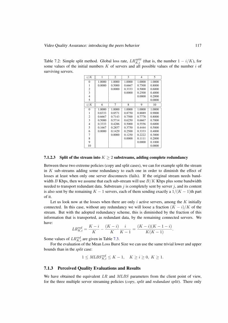
Video Quality Assurance: introducing the peers behavior 117
Table 7.2: Simple split method. Global loss rate, LRsplitK,i (that is, the number 1 − i/K), for
some values of the initial numbers K of servers and all possible values of the number i ofsurviving servers.
i/K 1 2 3 4 5
0 1.0000 1.0000 1.0000 1.0000 1.00001 0.0000 0.5000 0.6667 0.7500 0.80002 0.0000 0.3333 0.5000 0.60003 0.0000 0.2500 0.40004 0.0000 0.20005 0.0000
i/K 6 7 8 9 10
0 1.0000 1.0000 1.0000 1.0000 1.00001 0.8333 0.8571 0.8750 0.8889 0.90002 0.6667 0.7143 0.7500 0.7778 0.80003 0.5000 0.5714 0.6250 0.6667 0.70004 0.3333 0.4286 0.5000 0.5556 0.60005 0.1667 0.2857 0.3750 0.4444 0.50006 0.0000 0.1429 0.2500 0.3333 0.40007 0.0000 0.1250 0.2222 0.30008 0.0000 0.1111 0.20009 0.0000 0.1000
10 0.0000
7.1.2.3 Split of the stream into K ≥ 2 substreams, adding complete redundancy
Between these two extreme policies (copy and split cases), we can for example split the streamin K sub-streams adding some redundancy to each one in order to diminish the effect oflosses at least when only one server disconnects (fails). If the original stream needs band-width B Kbps, then we assume that each sub-stream will use B/K Kbps plus some bandwidthneeded to transport redundant data. Substream j is completely sent by server j, and its contentis also sent by the remaining K − 1 servers, each of them sending exactly a 1/(K − 1)th partof it.
Let us look now at the losses when there are only i active servers, among the K initiallyconnected. In this case, without any redundancy we will loose a fraction (K − i)/K of thestream. But with the adopted redundancy scheme, this is diminished by the fraction of thisinformation that is transported, as redundant data, by the remaining connected servers. Wehave:
LRredK,i =
K − iK
− (K − i)K
i
K − 1=
(K − i)(K − 1− i)K(K − 1)
.
Some values of LRredK,i are given in Table 7.3.
For the evaluation of the Mean Loss Burst Size we can use the same trivial lower and upperbounds than in the split case:
1 ≤ MLBS redK,i ≤ K − 1, K ≥ i ≥ 0, K ≥ 1.
7.1.3 Perceived Quality Evaluations and Results
We have obtained the equivalent LR and MLBS parameters from the client point of view,for the three multiple server streaming policies (copy, split and redundant split). There only

118 Optimal Quality in Multi-Source Streaming
Table 7.3: Split method with redundancy. Global loss rate, LRredK,i, for some values of the initial
numbers K of servers and all possible values of the number i of surviving servers.i/K 1 2 3 4 5
0 1.0000 1.0000 1.0000 1.0000 1.00001 0.0000 0.0000 0.3333 0.5000 0.60002 0.0000 0.0000 0.1667 0.30003 0.0000 0.0000 0.10004 0.0000 0.00005 0.0000
i/K 6 7 8 9 10
0 1.0000 1.0000 1.0000 1.0000 1.00001 0.6667 0.7143 0.7500 0.7778 0.80002 0.4000 0.4762 0.5357 0.5833 0.62223 0.2000 0.2857 0.3571 0.4167 0.46674 0.0667 0.1429 0.2143 0.2778 0.33335 0.0000 0.0476 0.1071 0.1667 0.22226 0.0000 0.0000 0.0357 0.0833 0.13337 0.0000 0.0000 0.0278 0.06678 0.0000 0.0000 0.02229 0.0000 0.000010 0.0000
remains to evaluate the PSQA simple function (of Section 5.2) mapping these two parametersinto perceived quality.
Sending K copies of the stream. Using the loss model for the copy method of Subsec-tion 7.1.2.1, we evaluate the PSQA measure in the different LRcopy
K,i possibilities, the result issummarized in Table 7.4.
Simple split of the stream into K ≥ 2 substreams. Using the loss model for the splitmethod of Subsection 7.1.2.2, we evaluate the PSQA measure in the different LRsplit
K,i pos-sibilities, the result is summarized in Table 7.5 for the lower quality bound (based in lowerbound MLBS split
K,i = 1) and in Table 7.6 for the upper quality bound (based in upper bound
MLBS splitK,i = K − i).
Split of the stream into K ≥ 2 substreams, adding complete redundancy, r = 1. Usingthe loss model for the redundant split method of Subsection 7.1.2.3, we evaluate the PSQAmeasure in the different LRred
K,i possibilities, the result is summarized in Table 7.7 for the lowerquality bound (based in lower bound MLBS red
K,i = 1) and in Table 7.8 for the upper qualitybound (based in upper bound MLBS red
K,i = K − i).

Video Quality Assurance: introducing the peers behavior 119
Table 7.4: Copy method. Perceived Quality as a function of K (initial number of servers) andi (number of surviving servers).
i/K 1 2 3 4 5
0 0.000 0.000 0.000 0.000 0.0001 10.000 10.000 10.000 10.000 10.0002 10.000 10.000 10.000 10.0003 10.000 10.000 10.0004 10.000 10.0005 10.000
i/K 6 7 8 9 10
0 0.000 0.000 0.000 0.000 0.0001 10.000 10.000 10.000 10.000 10.0002 10.000 10.000 10.000 10.000 10.0003 10.000 10.000 10.000 10.000 10.0004 10.000 10.000 10.000 10.000 10.0005 10.000 10.000 10.000 10.000 10.0006 10.000 10.000 10.000 10.000 10.0007 10.000 10.000 10.000 10.0008 10.000 10.000 10.0009 10.000 10.000
10 10.000
7.1.3.1 Assuring Video Quality
The PSQA technique makes it possible to know the subjective quality associated with everystate of the network (i.e, with any combination of working and failed servers). This informa-tion allows us to answer different interesting and relevant questions.
Under the given assumptions, the worst situation is just before a network rebuilds the bro-ken connections, that is, at time T− (if we consider that the last re-configuration happened attime 0). The expected perceived quality (considering the whole client population) at that timeis then
E(QK) =K∑i=1
Q(LRK,i,MLBSK,i)pK,i(T ),
where Q() is the PSQA simple function of Section 5.2.Table 7.9 and Figure 7.2 show the values of E(QK) for the three policies, for K varying
from 1 to 10 (the data was computed using the lower bound for the perceived quality, the dif-ference with the upper bound is completely negligible). Observe that, as it should be expected,the expected value is close to the maximal one (10), for any number of servers. We can ob-serve also that there is a slight trend towards smaller values as K increases. This is due tothe fact that the probability of having at least a failure (a missing flow) before T increases asK increases (this probability is 1 − e−KλT ). This compensates the effect of increasing thenumber of flows, and with the (realistic) numerical values used here, the combined effect isthis decreasing trend. In the case where there is no redundancy (simple split), the subjectivequality degenerates rapidly with the growth of serversK. In the redundant split policy, passingfrom one server to two servers improves greatly the quality levels; adding additional serverscan lead to slight decreases in perceived quality, but the behavior is very robust in this aspect.

120 Optimal Quality in Multi-Source Streaming
Table 7.5: Simple split method. Minimal Perceived Quality (MLBS splitK,i = 1) as a function of
K (initial number of servers) and i (number of surviving servers).i/K 1 2 3 4 5
0 0.000 0.000 0.000 0.000 0.0001 10.000 0.051 0.045 0.045 0.0452 10.000 0.075 0.051 0.0453 10.000 0.099 0.0634 10.000 0.1235 10.000
i/K 6 7 8 9 10
0 0.000 0.000 0.000 0.000 0.0001 0.045 0.045 0.045 0.045 0.0452 0.045 0.045 0.045 0.045 0.0453 0.051 0.045 0.045 0.045 0.0454 0.075 0.059 0.051 0.046 0.0455 0.146 0.087 0.067 0.057 0.0516 10.000 0.168 0.099 0.075 0.0637 10.000 0.190 0.111 0.0838 10.000 0.212 0.1239 10.000 0.23310 10.000
Table 7.6: Simple split method. Maximal Perceived Quality (MLBS splitK,i = K−i) as a function
of K (initial number of servers) and i (surviving servers).i/K 1 2 3 4 5
0 0.000 0.000 0.000 0.000 0.0001 10.000 0.051 0.075 0.097 0.1132 10.000 0.075 0.085 0.0973 10.000 0.099 0.1054 10.000 0.1235 10.000
i/K 6 7 8 9 10
0 0.000 0.000 0.000 0.000 0.0001 0.126 0.136 0.145 0.152 0.1582 0.113 0.126 0.136 0.145 0.1523 0.109 0.113 0.126 0.136 0.1454 0.126 0.127 0.127 0.128 0.1365 0.146 0.146 0.144 0.143 0.1426 10.000 0.168 0.165 0.162 0.1587 10.000 0.190 0.185 0.1798 10.000 0.212 0.2059 10.000 0.23310 10.000
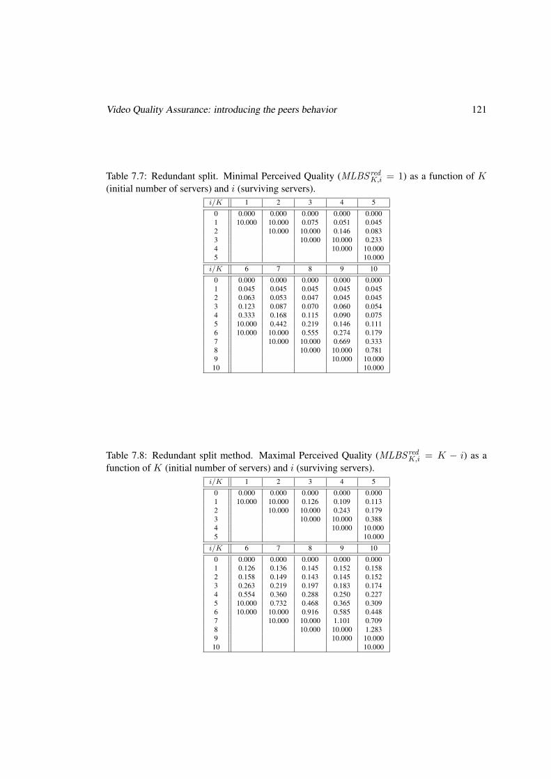
Video Quality Assurance: introducing the peers behavior 121
Table 7.7: Redundant split. Minimal Perceived Quality (MLBS redK,i = 1) as a function of K
(initial number of servers) and i (surviving servers).i/K 1 2 3 4 5
0 0.000 0.000 0.000 0.000 0.0001 10.000 10.000 0.075 0.051 0.0452 10.000 10.000 0.146 0.0833 10.000 10.000 0.2334 10.000 10.0005 10.000
i/K 6 7 8 9 10
0 0.000 0.000 0.000 0.000 0.0001 0.045 0.045 0.045 0.045 0.0452 0.063 0.053 0.047 0.045 0.0453 0.123 0.087 0.070 0.060 0.0544 0.333 0.168 0.115 0.090 0.0755 10.000 0.442 0.219 0.146 0.1116 10.000 10.000 0.555 0.274 0.1797 10.000 10.000 0.669 0.3338 10.000 10.000 0.7819 10.000 10.000
10 10.000
Table 7.8: Redundant split method. Maximal Perceived Quality (MLBS redK,i = K − i) as a
function of K (initial number of servers) and i (surviving servers).i/K 1 2 3 4 5
0 0.000 0.000 0.000 0.000 0.0001 10.000 10.000 0.126 0.109 0.1132 10.000 10.000 0.243 0.1793 10.000 10.000 0.3884 10.000 10.0005 10.000
i/K 6 7 8 9 10
0 0.000 0.000 0.000 0.000 0.0001 0.126 0.136 0.145 0.152 0.1582 0.158 0.149 0.143 0.145 0.1523 0.263 0.219 0.197 0.183 0.1744 0.554 0.360 0.288 0.250 0.2275 10.000 0.732 0.468 0.365 0.3096 10.000 10.000 0.916 0.585 0.4487 10.000 10.000 1.101 0.7098 10.000 10.000 1.2839 10.000 10.000
10 10.000
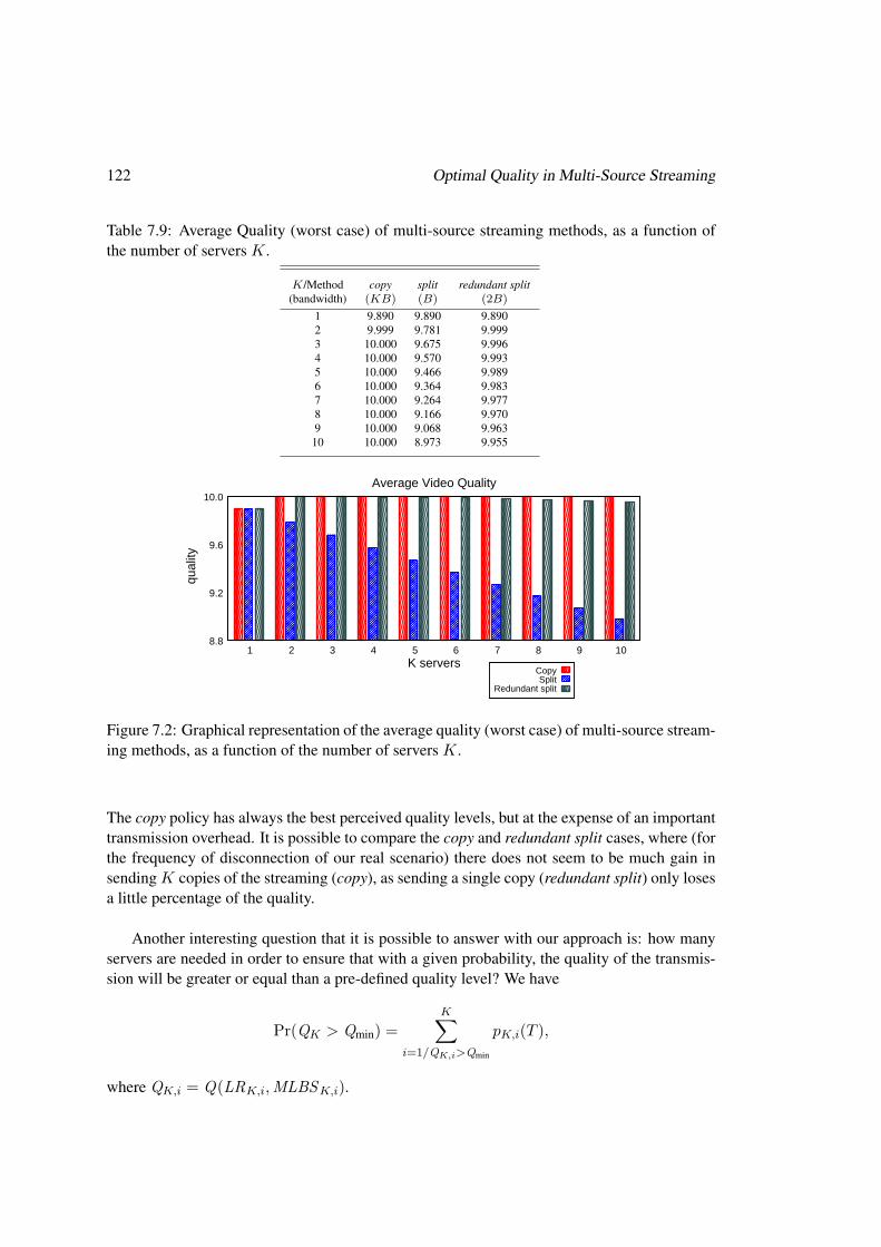
122 Optimal Quality in Multi-Source Streaming
Table 7.9: Average Quality (worst case) of multi-source streaming methods, as a function ofthe number of servers K.
K/Method copy split redundant split(bandwidth) (KB) (B) (2B)
1 9.890 9.890 9.8902 9.999 9.781 9.9993 10.000 9.675 9.9964 10.000 9.570 9.9935 10.000 9.466 9.9896 10.000 9.364 9.9837 10.000 9.264 9.9778 10.000 9.166 9.9709 10.000 9.068 9.963
10 10.000 8.973 9.955
8.8
9.2
9.6
10.0
1 2 3 4 5 6 7 8 9 10
qual
ity
K servers
Average Video Quality
CopySplit
Redundant split
Figure 7.2: Graphical representation of the average quality (worst case) of multi-source stream-ing methods, as a function of the number of servers K.
The copy policy has always the best perceived quality levels, but at the expense of an importanttransmission overhead. It is possible to compare the copy and redundant split cases, where (forthe frequency of disconnection of our real scenario) there does not seem to be much gain insendingK copies of the streaming (copy), as sending a single copy (redundant split) only losesa little percentage of the quality.
Another interesting question that it is possible to answer with our approach is: how manyservers are needed in order to ensure that with a given probability, the quality of the transmis-sion will be greater or equal than a pre-defined quality level? We have
Pr(QK > Qmin) =K∑
i=1/QK,i>Qmin
pK,i(T ),
where QK,i = Q(LRK,i,MLBSK,i).

Improving the Multi-Source Streaming and Looking for Optimality: Considering the peers’ heterogeneity123
Table 7.10: Pr(QK > 9.99) in our multi-source streaming methods, as a function of thenumbers K of servers.
K/Method copy split redundant split(bandwidth) (KB) (B) (2B)
1 0.988950 0.988950 0.9889502 0.999878 0.978023 0.9998783 0.999999 0.967216 0.9996364 ∼1.000000 0.956529 0.9992785 ∼1.000000 0.945959 0.9988066 ∼1.000000 0.935507 0.9982227 ∼1.000000 0.925170 0.9975298 ∼1.000000 0.914947 0.9967299 ∼1.000000 0.904837 0.995826
10 ∼1.000000 0.894839 0.994820
Assume we want to ensure a perfect quality (Qmin = 9.99). Table 7.10 gives Pr(QK >9.99) for different values of K, in the three streaming policies. For instance, if we wantPr(QK > 9.99) ≥ 0.999 (an alternative equivalent interpretation is that we want to ensurethat at least 99.9% of the users will perceive perfect quality), this table says that, this can beachieved if at least 2 servers are used in the copy method; or if between 2 and 4 servers are usedin the redundant split method. The condition is impossible to satisfy if there is no redundancyat all (that is, with the simple split method).
This study suggests that among the different policies for multi-source streaming techniques,the ones employing a limited amount of redundancy may well be the methods of choice, as theyallow to improve the QoE at the expense of a limited transmission overhead. Simple analyticalmodels can be useful to understand the qualitative and quantitative behavior of the differentpolicies. In order to support the designers’ decision making, it can be useful to develop morerealistic models; in particular, next section introduces the peers dynamics heterogeneity, amongother improvements.
7.2 Improving the Multi-Source Streaming and Looking for Opti-mality: Considering the peers’ heterogeneity
It has been shown that peers are heterogeneous in their capability [299] and a network designhas to consider this behavior to be scalable. The election of the peer servers that are part of themulti-source streaming is important, with respect to their bandwidth capacity, and especiallyto their lifetime.
In our approach, the P2P system has the necessary knowledge about the peers and thenetwork state, and can thus decide which peer will serve which other node (see Chapter 8 for thestructural P2P design problem), and how flows must be split and merged. The network topologyis then re-built periodically, every T seconds, with T = 10 seconds as well as the previoussection. A generic peer starts the cycle by receiving the video stream from K heterogeneousand independent server peers, but before T some server peers can become disconnected.

124 Optimal Quality in Multi-Source Streaming
In this section we will describe some improvements on the multi-source streaming scheme,on the models, and how we use them for deriving optimality results. These improvementsgo in the direction of sending the most important data from peers highly “engaged” with thenetwork. All the improvements described here were implemented (Section 10.1) and tested(Section 10.3) on our GOL!P2P prototype.
7.2.1 First improvement of the scheme: unequal splitting
Instead of splitting into sub-streams with equal bandwidth, we send a fraction yk of the streamby flow (server) k. We call yk the weight of server k. As we want that the best servers sendmost of the data, we set yk+1 = γyk, with γ > 1. This means that yk = γk−1y1, withy1 = (γ − 1)/(γK − 1).
We also add some redundancy r ∈ [0, 1] to the global flow; r = 0 means no redundancy,r = 1 means that any frame is sent twice. If the original stream has a bitrate of B Kbps, thetotal bandwidth employed is thus BW r = (1 + r)B Kbps. The redundancy is distributed inthe following way. A fraction r of the original data sent by server k is also sent by the otherservers, proportionally to their weights. The total bandwidth BW r
k used by server k is then
BW rk = ykB +
K∑j=1,j 6=k
rykByj
1− yk = (1 + r) ykB,
where rykByj/(1 − yk) is the bandwidth used by server k to stream the redundancy of sub-stream j. The technique implies that each frame is sent either once or twice, but no frame issent more than twice.
This improvement generalizes the split methods presented before, where split uses γ = 1+
and r = 0, and redundant split uses γ = 1+ and r = 1.
7.2.2 Improving the model of the peers’ dynamics
Concerning the model, we consider now that peers belong to different classes, according totheir mean connection time in the network (peer’s lifetime). The average behavior of the peersin each class is obtained from our video delivery reference service presented in Section 2.5.We proceed as follows. After choosing K, we sort the whole set of peers in the available logsaccording to their mean connection times. If M is the size of the population, the first M/Kpeers are assigned to class 1, the second M/K to class 2, etc. With class k we associate thefailure rate λk = 1/mk where mk is the mean connection time of the peers in class k, and wethen assume that in that class, peers remain connected for an exponentially distributed periodof time. Observe that λ1 ≥ λ2 ≥ · · · ≥ λK (best peers are at the end). The reason we use asmany classes as sub-streams is that we consider here that peers are all equivalent with respectto the service, so, that they must all receive the same service. This leads to the fact that eachclient is served (at the beginning of a cycle) by one server of each class.
Let us denote by Nk(t) the binary r.v. equal to 1 iff server k is connected at t, and by ~N(t)the vector ~N(t) = (N1(t), · · · , NK(t)). Then, for any configuration ~n ∈ {0, 1}K , we have
Pr( ~N(t) = ~n) =∏
j:nj=1
e−λjt∏
j:nj=0
(1− e−λjt). (7.1)
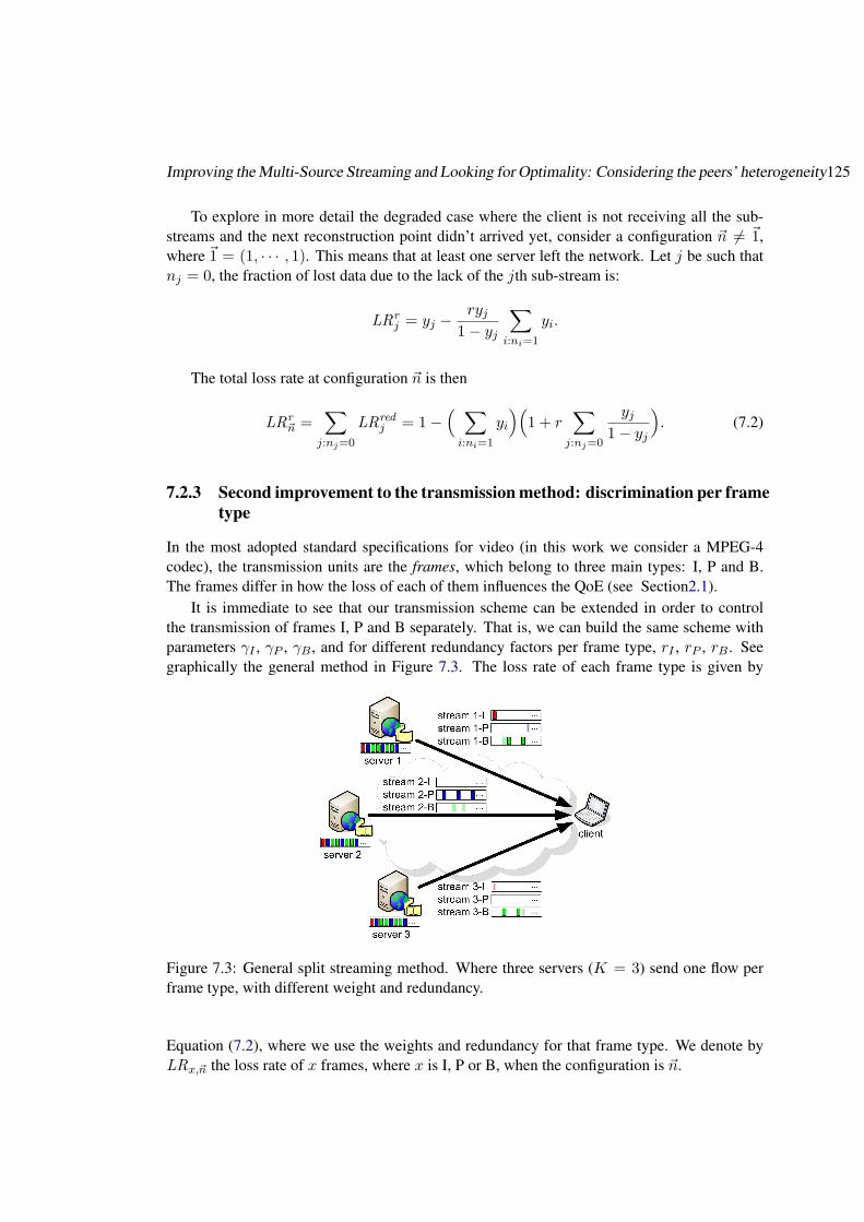
Improving the Multi-Source Streaming and Looking for Optimality: Considering the peers’ heterogeneity125
To explore in more detail the degraded case where the client is not receiving all the sub-streams and the next reconstruction point didn’t arrived yet, consider a configuration ~n 6= ~1,where ~1 = (1, · · · , 1). This means that at least one server left the network. Let j be such thatnj = 0, the fraction of lost data due to the lack of the jth sub-stream is:
LRrj = yj − ryj
1− yj∑i:ni=1
yi.
The total loss rate at configuration ~n is then
LRr~n =
∑j:nj=0
LRredj = 1−
( ∑i:ni=1
yi
)(1 + r
∑j:nj=0
yj1− yj
). (7.2)
7.2.3 Second improvement to the transmission method: discrimination per frametype
In the most adopted standard specifications for video (in this work we consider a MPEG-4codec), the transmission units are the frames, which belong to three main types: I, P and B.The frames differ in how the loss of each of them influences the QoE (see Section2.1).
It is immediate to see that our transmission scheme can be extended in order to controlthe transmission of frames I, P and B separately. That is, we can build the same scheme withparameters γI , γP , γB , and for different redundancy factors per frame type, rI , rP , rB . Seegraphically the general method in Figure 7.3. The loss rate of each frame type is given by
Figure 7.3: General split streaming method. Where three servers (K = 3) send one flow perframe type, with different weight and redundancy.
Equation (7.2), where we use the weights and redundancy for that frame type. We denote byLRx,~n the loss rate of x frames, where x is I, P or B, when the configuration is ~n.

126 Optimal Quality in Multi-Source Streaming
Using now the PSQA complex function, of Section 5.3.3, giving the perceived quality as afunction of the per-frame type loss rates1 , the QoE in that configuration is Q(LRI,~n, LRP,~n, LRB,~n).We fix the motion source parameters of the original function to its average values (the averageGOP size is 174 frames, and the P-Frames Weight per GOP is 0.7007), because we do not usethem in this analysis.
Our main objective here is to maximize the mean QoE value, considered at the end of thecycle (worst case analysis), and when at least one server is down, because this is the maincritical situation. This expectation is
E(QK)(T ) =∑~n6=~1
Pr( ~N(T ) = ~n)Q(LRI,~n, LRP,~n, LRB,~n),
where the peer’s probability connection for each configuration is defined by Equation (7.1).
7.2.4 Optimization Results
In what follows, we analyze the behavior of the system when at least one peer leaves thenetwork, in order to address the robustness of our proposal. The presented results focus onthe evaluation of all concerned parameters for maximizing E(QK)(T ). The needed bandwidthfor delivering the original video is B = 512 Kbps. We will consider three redundancy levels:0%, 25% and 50%. In the two last cases, the total bandwidth is equal to 640 and 768 Kbpsrespectively.
The optimization results were obtained using the fminsearch function of Matlab2, whichfinds the minimum of a scalar function of several variables, starting at an initial estimation. Forall the results, we randomly chose 10 starting points, with 2 ≤ K ≤ 10, and the maximummean quality among all provided results was selected.
For the scenario we are considering, first observe that if we have only one server peerand it leaves the network, the QoE is obviously zero. Now, in real systems, peers have some-times bandwidth constraints. We will consider two cases: either the peers upload informationwithout bandwidth constraints (i.e. only the download bandwidth received by the client isconstrained by BW r = (1 + r)B Kbps), or the upload bandwidth is restricted to less thanBW r/K Kbps. The two scenarios result in different restrictions on the γ and r parametervalues. The fminsearch function does not consider constraints, we augmented the objectivefunction with bandwidth constraints in each case in order to solve it in Matlab.
No upload bandwidth limitations. We start by the simple case, where the bandwidth islimited only by its total amount, without caring about the bandwidth of each server peer. Wereport our results on Tables 7.11, 7.12 and 7.13 (r = 0%, r = 25% and r = 50%).
Equal upload bandwidth limitation. Now, consider that each server peer has a bandwidthlimitation. Tables 7.14 and 7.15 show the results (r = 25% and r = 50%).
The following conclusions can be listed. (1) As expected, more bandwidth results in a bet-ter quality for the delivered video. (2) For P-frames, the largest quality is achieved when γP is
1This function shows that the quality degrades quickly with an increment in the loss rate of frames I and P, andthat the impact of P-frames’ losses is a bit higher than for I-frames. Also, it shows that the quality degrades slowlywith an increment in the loss rate of B-frames.
2© 1984-2007 The MathWorks, Inc.

Improving the Multi-Source Streaming and Looking for Optimality: Considering the peers’ heterogeneity127
around 2. This means that server peers that stay longer in the system will be responsible for de-livering the most important information. These results match with practical experiences, whereP-frames have a crucial role on the quality perceived by the end-user. (3) After the P-frame inimportance order with respect to the quality, we have I-frames and then B-frames, confirmingthe results of the subjective testing sessions. (4) The redundancy value is counterbalanced bythe γ value: for greater γ we can use a smaller value of the redundancy factor, with the follow-ing interpretation: if the largest part of the information is delivered by the most stable peers, itis not necessary to use a high redundancy factor.
To explore the robustness of the optimization procedure, we selected some cases with morestarting points in order to obtain the best E(QK)(T ). Just for illustration, let us consider thecase with r = 25% and K = 2 (Table 7.12). We randomly chose 70 starting points leadingto 70 values of E(QK)(T ) ranging in [2.571, 3.716] with an arithmetic average value of 3.250.Coming back to Table 7.12, we can see that this does not basically change our pseudo-optimalpoints.
The analysis shows that the highest the number of server peers, the better the quality. On theother hand, the signaling overhead also increases with that number. The results show, however,that a few number of servers is enough for an excellent quality level (e.g., for E(QK)(T ) ≥ 9.0and 25% of redundancy, 7 servers are enough). In Section 10.1, we discuss about the mainproblems of implementing the multi-source streaming technique and the practical effects ofincreasing the number of server peers.
Table 7.11: Multi-source configurations without upload bandwidth limitations, γ and redun-dancy factors optimization (0% redundancy)
K E(QK)(T ) γI γP γB
1 0 - - -2 2.471 1.999e+00 2.000e+00 1.999e+003 4.368 1.999e+00 2.000e+00 1.999e+004 6.041 1.997e+00 1.999e+00 1.999e+005 7.297 1.999e+00 1.999e+00 1.993e+006 8.159 2.000e+00 1.999e+00 1.999e+007 8.727 1.999e+00 2.000e+00 1.999e+008 9.099 1.999e+00 1.999e+00 1.999e+009 9.346 1.999e+00 1.999e+00 1.999e+0010 9.477 1.999e+00 2.000e+00 1.999e+00
K E(QK)(T ) rI rP rB
1 0 - - -2 2.471 8.554e-02 1.942e-02 8.535e-023 4.368 3.852e-02 4.085e-02 3.455e-024 6.041 9.749e-02 1.904e-02 7.325e-025 7.297 1.607e-02 4.961e-02 8.200e-036 8.159 8.506e-02 2.005e-02 8.160e-037 8.727 8.642e-02 2.009e-02 7.965e-028 9.099 8.749e-02 2.000e-02 7.898e-029 9.346 9.477e-02 4.007e-02 1.867e-0210 9.477 8.046e-02 3.937e-02 9.900e-04

128 Optimal Quality in Multi-Source Streaming
Table 7.12: Multi-source configurations without upload bandwidth limitations, γ and redun-dancy factors optimization (25% redundancy)
K E(QK)(T ) γI γP γB
1 0 - - -2 3.493 1.189e+00 1.999e+00 1.146e+003 5.593 1.000e+00 1.999e+00 1.712e+004 7.016 1.535e+00 1.992e+00 1.999e+005 7.857 1.000e+00 1.999e+00 1.589e+006 8.606 1.524e+00 1.995e+00 1.744e+007 9.076 1.109e+00 1.999e+00 1.921e+008 9.332 1.000e+00 1.999e+00 1.993e+009 9.479 1.890e+00 1.999e+00 1.999e+00
10 9.591 1.999e+00 1.999e+00 1.898e+00
K E(QK)(T ) rI rP rB
1 0 - - -2 3.493 9.797e-01 2.547e-01 2.171e-013 5.593 9.999e-01 2.942e-01 8.694e-024 7.016 9.999e-01 2.252e-01 2.941e-015 7.857 9.223e-01 3.228e-01 1.491e-066 8.606 9.378e-01 2.789e-01 6.931e-067 9.076 9.949e-01 2.583e-01 4.065e-048 9.332 9.991e-01 2.154e-01 8.857e-029 9.479 9.999e-01 1.366e-01 9.171e-02
10 9.591 9.999e-01 1.829e-01 6.647e-02
Table 7.13: Multi-source configurations without upload bandwidth limitations, γ and redun-dancy factors optimization (50% redundancy)
K E(QK)(T ) γI γP γB
1 0 - - -2 5.011 1.258e+00 1.874e+00 1.615e+003 6.636 1.147e+00 1.863e+00 1.999e+004 7.865 1.999e+00 1.999e+00 1.999e+005 8.711 1.420e+00 1.993e+00 1.993e+006 9.024 1.644e+00 1.999e+00 1.601e+007 9.324 1.809e+00 1.999e+00 1.999e+008 9.610 1.999e+00 1.999e+00 1.998e+009 9.669 1.822e+00 1.995e+00 1.999e+00
10 9.766 1.910e+00 1.999e+00 1.914e+00
K E(QK)(T ) rI rP rB
1 0 - - -2 5.011 9.999e-01 6.629e-01 4.926e-063 6.636 9.999e-01 5.739e-01 3.093e-014 7.865 7.043e-01 6.323e-01 1.456e-015 8.711 9.999e-01 5.662e-01 3.887e-016 9.024 9.999e-01 4.340e-01 8.044e-017 9.324 5.996e-01 5.650e-01 5.259e-018 9.610 7.697e-01 6.520e-01 1.957e-019 9.669 4.824e-01 7.285e-01 4.523e-04
10 9.766 8.409e-01 7.082e-01 6.855e-06

Improving the Multi-Source Streaming and Looking for Optimality: Considering the peers’ heterogeneity129
Table 7.14: Multi-source configurations with upload bandwidth limitations, γ and redundancyfactors Optimization (25% Redundancy)
K E(QK)(T ) γI γP γB
1 0 - - -2 3.557 1.000e+00 1.960e+00 1.607e+003 5.442 1.296e+00 1.999e+00 1.771e+004 7.020 1.108e+00 1.999e+00 1.999e+005 7.972 1.220e+00 1.999e+00 1.797e+006 8.719 1.999e+00 1.997e+00 1.999e+007 9.064 1.409e+00 1.999e+00 1.661e+008 9.319 1.999e+00 1.999e+00 1.692e+009 9.510 1.995e+00 1.932e+00 1.974e+0010 9.586 1.999e+00 1.996e+00 1.949e+00
K E(QK)(T ) rI rP rB
1 0 - - -2 3.557 9.913e-01 2.953e-01 5.410e-043 5.442 9.999e-01 1.705e-01 4.744e-014 7.020 9.999e-01 2.279e-01 2.610e-015 7.972 9.999e-01 1.988e-01 3.856e-016 8.719 8.286e-01 3.305e-01 9.977e-067 9.064 9.999e-01 2.462e-01 2.373e-018 9.319 8.124e-01 2.946e-01 6.276e-069 9.510 7.986e-01 3.428e-01 5.984e-0510 9.586 1.550e-01 3.959e-01 4.255e-02
Table 7.15: Multi-source configurations with upload bandwidth limitations, γ and redundancyfactors Optimization (50% Redundancy)
K E(QK)(T ) γI γP γB
1 0 - - -2 4.787 1.000e+00 1.909e+00 1.000e+003 6.999 1.088e+00 1.991e+00 1.850e+004 7.865 1.999e+00 1.999e+00 1.999e+005 8.711 1.420e+00 1.993e+00 1.993e+006 9.188 1.273e+00 1.999e+00 1.761e+007 9.470 1.495e+00 1.998e+00 1.896e+008 9.610 1.999e+00 1.999e+00 1.998e+009 9.669 1.822e+00 1.995e+00 1.999e+0010 9.752 1.999e+00 1.967e+00 1.655e+00
K E(QK)(T ) rI rP rB
1 0 - - -2 4.787 9.929e-01 6.576e-01 4.480e-033 6.999 9.999e-01 6.552e-01 1.138e-014 7.865 7.043e-01 6.323e-01 1.456e-015 8.711 9.999e-01 5.662e-01 3.887e-016 9.188 9.810e-01 6.599e-01 1.057e-017 9.470 9.999e-01 6.222e-01 1.825e-018 9.610 7.697e-01 6.520e-01 1.957e-019 9.669 4.824e-01 7.285e-01 4.523e-0410 9.752 9.574e-01 6.826e-01 1.589e-05

130 Optimal Quality in Multi-Source Streaming
7.3 Assuring Quality at the Receiver: buffering protection
In this section we study the protection strategies that a client is enable to use in a network withserver failures in order to improve (and also ensure) a quality level. This analysis is from theclient point of view, where it is not possible to change the network behavior. In particular, wediscuss about the client buffer size to protect it of a server disconnection. It hardly depends onthe network topology rebuild strategy, so, our analysis is done for different rebuild scenarios.Because of mathematical issues, we limit the concluded analytical expression of the buffer sizeto the case with only one server; we are working in a extension for the multi-source approach.
We are interested here in the impact of the disconnection failures on the quality of thestream as seen by the clients. The traditional way of analyzing this is to study performancemeasures of the systems, or dependability ones. Here, we will follow a performability-likeapproach, considering at the same time the failures (as defined before) and the resulting per-formance. However, instead of looking at standard metrics which we qualify here of indirect(loss rates, delays, or reliability, availability...), we will address the ultimate target, the qualityof the stream, as perceived by the end user, using PSQA.
We show a possible use of the PSQA minimal closed-form function of Subsection 5.2.4.It is rational function Q() of the chosen variables (here, LR and MLBS ), mapping them intoa MOS-like quality value. This means that we are approximating the perceived quality at tby Q(LR(t),MLBS (t)) where LR(t) and MLBS (t) are instantaneous values obtained bymeasuring.
Recall that Q(LR,MLBS ) has here the following form (seen in Subsection 5.2.4):
Q(LR,MLBS ) =aLR + bMLBS
cLR + dMLBS + ν,
where a = 0.00142128, b = 0.47242076, c = 0.00142128, d = 0.47242076 and ν = 0.01. InFigure 5.8 we can see this function, for the valid specific range of the input variables.
7.3.1 Buffering Model
We will use a simple model in order to study the way quality would be perceived in such asystem. For now, we will consider the streaming from a single source. Consider the followingsimplifying assumptions. The time to process a data unit (a frame) is exponentially distributedwith parameter µ. The arrival rate of frames to the client, when the node sending them to itis working, is obviously also µ. The client starts with a buffer containing N frames. Wheneverything goes correctly, he receives frames at the same rate he plays them, so (we assume)the buffer level will remain constant. The node sending the frames can fail (typically, it willleave the network), which happens with some failure rate λ (that is, we assume an exponen-tially distributed sojourn time of a peer in the network). The network reconfigurates itself atpoints in time distributed as a Poisson process with rate f = 1/T . After a reconfiguration (aninstantaneous action, in our model), the clients that had lost their stream because of a failure areconnected again (to some peer/source). Let us call cycle the period between two consecutivenetwork reconfigurations.

Assuring Quality at the Receiver: buffering protection 131
With the usual independence assumptions, we can build the following Markov process Xdescribing the evolution of such a client, during a cycle. The state space is the set of non-negative integers. State 0 means that the node sending the frames to the observed client (fromnow, the server peer) is active, and everything goes normally. The client’s buffer level is N .If the server fails, X moves to state 1 (with rate λ). State n, for 1 ≤ n ≤ N + 1 means thatthe server is down (left the system) and that the client has already played n− 1 frames in thatsituation; the number of frames remaining in the buffer isN−n+1. StateN+m,m ≥ 1 meansthat the server is down and that the client has already lostm−1 frames (because their playtimesarrived and there was nothing to play). Figure 7.4 shows the transition diagram of process X .The loop at state 0 represents the fact that there is a regeneration of the whole network withrate f . Of course, if the client started with N frames in its buffer, after the next reconfigurationit will have a random number Y of frames, Y ≤ N . We will look at that later. For the moment,we will use X to compute the loss rate at the client side. We call this a performability modelbecause it takes into account failures, repairs, and services. Let πn denote the probability that
... ... ...ff f
f f f
µ µ µ µ µ µ µ0 1 2 n N N+1
λ
Figure 7.4: Evolution of a client during a cycle.
X is at state n in steady state. Then, the loss rate in the cycle will be defined as the probabilityof being at states N + 1, N + 2, etc. (which is, due to the PASTA property, the probability thatat the moment we must play a frame, there is no frame in the buffer). In formal terms,
LR =∑
n≥N+1
πn.
Process X is always stable, and we have
π0 =1
1 + ε, ε =
λ
f,
π1 =π0
1 + δ, δ =
f
µ
and for any n ≥ 2,
πn =ε
1 + ε
δ
(1 + δ)n.
After some algebra, this leads to
LR =ε
1 + ε
1(1 + δ)N
.

132 Optimal Quality in Multi-Source Streaming
The computation of the MLBS is easier. First, we are now counting, so, we work on thecanonical discrete time Markov chain embedded into X . In Figure 7.5 we see its transitionprobabilities. The parameters of this model are
... ... ...vq q
q q q
p p p p p p p0 1 2 n N N+1
u
Figure 7.5: The canonical discrete time Markov chain embedded in X .
u =ε
1 + ε, v = 1− u, p =
11 + δ
, q = 1− p.
The probability that a burst of losses has size j being pj−1q, we have:
MLBS =1q
= 1 +µ
f.
Observe that if the cycle starts with N frames in the buffer, at the beginning of next cyclethe buffer can contain N , N − 1, ..., frames. We denoted by Y the number of frames presentin the buffer at the beginning of next cycle. We have
Pr(Y = N) = v + uq,
then, for j = N − 1, N − 2, · · · , 1,
Pr(Y = j) = upN−jq,
and, finally,Pr(Y = 0) = upN .
7.3.2 Buffering Protection Strategy
The main objective is to analyze how different sojourn times of a peer in the network, as wellas different reconfiguration strategies, affect the quality of the video played by a client; and toreact to this situation choosing an adequate buffer size in order to ensure a quality level.
We consider here two strategies of network rebuilding. In the first case, every T = 1/fsecs, on the average, the network is reconstructed. By means on message exchanges, the systemdiscovers which nodes left and, if they were serving other peers, they replace them by othernodes to allow the former to continue receiving the signal. In the second case, we consider

Assuring Quality at the Receiver: buffering protection 133
using a supplementary server peer that delivers the information to the client having lost itssource until the network can be reconfigured.
Let us analyze the first scenario. We will consider two cases here: when a cycle begins theclient has either 0 or 100 frames in the buffer. For the failure rate, we consider a broad range:λ = 0.1, 0.01, 0.001. Figure 7.6 shows the values for the loss rate metric in these scenarios asa function of the reconfiguration rate f , in a range from 1 sec to 20 sec (larger reconfigurationintervals decrease significantly the network performance). As expected, if the server spendsmore time in the network, the client observes less losses. A similar correlation can be observedwith respect to the initial number of frames in the buffer: the larger this number, the smallerthe loss rate.
1e-05
1e-04
0.001
0.01
0.1
1
0 0.1 0.2 0.3 0.4 0.5 0.6 0.7 0.8 0.9 1
loss
rat
e
reconfiguration rate
Loss Rate
B = 0
B = 0
B = 0
B = 100
B = 100
B = 100
λ = 0.1
λ = 0.01
λ = 0.001
Figure 7.6: Loss rate, LR, measure for the first strategy of reconfiguration.
Now, let us consider the MLBS metric. For the set of values of λ and f , the MLBS reacheshigh values (600 to 30 frames). In these cases, we are out of the input domain of Q(). Whatsimply happens is that such high values of MLBS mean that quality will be very low (just 30frames correspond to a second of signal). Moreover, observe that those very long bursts arerare. The probability of observing at least m consecutive losses is upN+m in the case of abuffer having at the beginning of the cycle N frames, that is, ε(1 + ε)−1(1 + δ)−N−m. Thismeans that a very few number of peers will observe those bursts, leading to a poor quality. Inother words, the situation where MLBS = 600 corresponds to a case of very rare losses, butwhen happening, arriving in long bursts.
In any case, a reconfiguration rate f = 0.1 means a mean reconfiguration period of T = 10sec., and f = 1 means a reconfiguration every sec, on the average. This can be too low. Inorder to improve the performance of the system, let us consider the use of a special server peerthat sends the stream to nodes having lost their servers, before the next reconfiguration pointarrives. Let us consider that the mean time to such a special server starts transmitting infor-mation is 250 msec. In this case, as expected, the loss rate and the MLBS are lower than inthe previous one. Again we consider two different initial buffer sizes in the cycle: either 0 or

134 Optimal Quality in Multi-Source Streaming
100 frames, and the same range for the failure rate λ. The largest loss probability is equal to0.025 and the MLBS varies between 7 and 8.4, as shown in Figure 7.7. The LR and MLBS
6.8
7
7.2
7.4
7.6
7.8
8
8.2
8.4
8.6
4 4.1 4.2 4.3 4.4 4.5 4.6 4.7 4.8 4.9 5
mea
n lo
st b
urs
t si
ze
reconfiguration rate
Mean Lost Burst Size
Figure 7.7: MLBS measure for the second strategy of reconfiguration.
values were mapped into a perceived quality level using the Q() function. The resulting qualityQ had a small variation in this context: the maximum quality is equal to 0.87 and the minimumquality is equal to 0.82. This means that in the considered situation, quality is good enough.
Using our model and the minimal Q() function introduced before, we can provide an an-alytical expression of the perceived quality as a function of the system’s parameters λ, f , Nand µ. Just replace LR and MLBS in (5.1) by the corresponding expressions provided by themodel.
This can allow to easily obtain rough answers to interesting questions. For instance, whichis the minimal buffer size necessary to assure a given quality level? That is, what is the minimalvalue of N such that Q(λ, f,N, µ) ≥ Q0? After some algebra, this leads to:
N ≥
logcQ0 − a(
1 +f
λ
)[(bQ0 − d)
(1 +
µ
f
)−Q0ν
]log(
1 +f
µ
) .
For Q0 = 0.87, it is possible to see that the necessary buffer size is very small, with amaximum of 28 frames (∼ 1 second) when we have λ = 0.1 and the highest reconfigurationrate f = 5.
In this section, we considered two network design parameters in our analysis: the reconfig-uration rate f of the network and the number N of frames in the buffer just after a reconfigura-tion. The coupling between PSQA and the performability model allows to evaluate the impactof f and N on the QoE. Current work is being done now to extend these results to multiplesources and to use transient views of the system.

Summary and Conclusions 135
7.4 Summary and Conclusions
This chapter proposes some transient models that may be useful for the design of a live-videoP2P distribution system following a multi-source procedure.
A first focus is on how to ensure a high QoE for the users, when simple multi-source poli-cies are used. Three policies are considered. In the first one, the original stream is entirely repli-cated and independently sent from K different servers. In the second one, the original streamis divided into K independent substreams, one per server, so that their union reconstructs theoriginal signal. In the third one, the original stream is also divided into K independent sub-streams, but at each stream some redundancy is added, so that the loss of any substream canbe recovered from the K − 1 remaining ones. To evaluate the different options, we developanalytical models for computing the loss process as functions of the total number of serversK and the number of servers in working order, for each of the cases. We also give a simpletransient Markovian model with an explicit analytical solution for computing the distributionof the number of working and failed servers at a given time T .
We then focused our analysis on how to maximize the delivered QoE of an improved multi-source technique based on the heterogeneous peers’ lifetimes. This improved technique pro-vides good quality to the end-users, mitigating the impact of losses coming from peers discon-nections. The main results concern the joint impact of different frame type losses on the QoE,using the PSQA methodology, and how to identify an optimal parameter setting, in order toobtain the best possible quality level for a given peers’ dynamics. This led to the method thatwe use in our prototype; the main objective was to provide a methodology that can be used inother P2P systems with similar constraints and users’ behavior, in order to set the best possibleQoE.
The QoE perceived by the end users is captured using different PSQA functions, showingthe applicability of the PSQA methodology to network design. The developed models areexperimentally evaluated using configurations computed from realistic parameters (computingusing information collected at our video delivery reference service).
The improved multi-source technique is applied at the server side of the network in orderto ensure an optimal delivery. In this chapter, we also study the protection strategy at the clientside. We present a simple Markov performability model combined with PSQA. The proposedmodel allows us to describe the evolution of a peer client during a cycle, i.e, the period betweentwo consecutive network reconfigurations. Using PSQA we are able to work with the perceivedquality as a function of the design parameters and thus to perform a quantitative analysis of oursystem.

136 Optimal Quality in Multi-Source Streaming
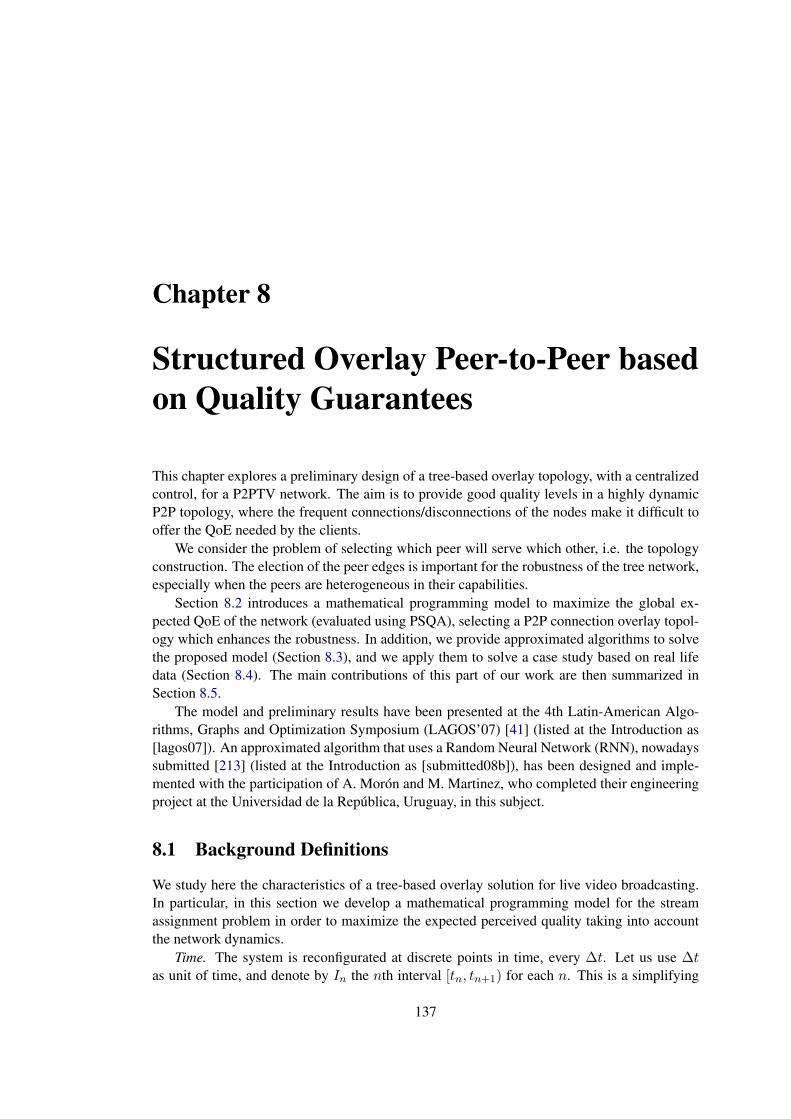
Chapter 8
Structured Overlay Peer-to-Peer basedon Quality Guarantees
This chapter explores a preliminary design of a tree-based overlay topology, with a centralizedcontrol, for a P2PTV network. The aim is to provide good quality levels in a highly dynamicP2P topology, where the frequent connections/disconnections of the nodes make it difficult tooffer the QoE needed by the clients.
We consider the problem of selecting which peer will serve which other, i.e. the topologyconstruction. The election of the peer edges is important for the robustness of the tree network,especially when the peers are heterogeneous in their capabilities.
Section 8.2 introduces a mathematical programming model to maximize the global ex-pected QoE of the network (evaluated using PSQA), selecting a P2P connection overlay topol-ogy which enhances the robustness. In addition, we provide approximated algorithms to solvethe proposed model (Section 8.3), and we apply them to solve a case study based on real lifedata (Section 8.4). The main contributions of this part of our work are then summarized inSection 8.5.
The model and preliminary results have been presented at the 4th Latin-American Algo-rithms, Graphs and Optimization Symposium (LAGOS’07) [41] (listed at the Introduction as[lagos07]). An approximated algorithm that uses a Random Neural Network (RNN), nowadayssubmitted [213] (listed at the Introduction as [submitted08b]), has been designed and imple-mented with the participation of A. Morón and M. Martinez, who completed their engineeringproject at the Universidad de la República, Uruguay, in this subject.
8.1 Background Definitions
We study here the characteristics of a tree-based overlay solution for live video broadcasting.In particular, in this section we develop a mathematical programming model for the streamassignment problem in order to maximize the expected perceived quality taking into accountthe network dynamics.
Time. The system is reconfigurated at discrete points in time, every ∆t. Let us use ∆tas unit of time, and denote by In the nth interval [tn, tn+1) for each n. This is a simplifying
137

138 Structured Overlay Peer-to-Peer based on Quality Guarantees
assumption, that allows to evaluate the main difficulties; in reality, a more continuous solutioncan be implemented.
Distribution scheme. The stream is originally sent to the clients (or terminals) by a brod-caster node s. Most clients act also as servers, relaying streams to other clients. For thispurpose, each node v has an available output bandwidth BW out
v . The system distributes asingle stream of live video by means of K sub-streams denoted by σ1, σ2, ..., σK . Each sub-stream σk is sent with a constant bandwidth bwk. The total bandwidth used to send the streamis∑K
k=1 bwk. When a client receives the K substreams, it reproduces the stream with per-fect quality. If it does not receive all the K substreams, it will reproduce a stream that canhave lower quality, depending on which substreams are received and which redundant schemeis used (the particular multi-source streaming technique used is presented in Chapter 7). Toevaluate the quality at the client side, we use the PSQA technology.
Dynamics. The evolution of the system from tn to (tn+1)− is as follows: some nodes leavein In, possibly disconnecting other clients in some substreams; at the same time, some nodesenter the network requesting for connection; they remain isolated from the rest of the nodesuntil tn+1 when the new reconfiguration action is performed. The goal of the reconfigurationis to reconnect the disconnected nodes and to connect the new arrivals to the network. Theconnexion scheme always builds trees of peers. At time (tn+1)−, just before the reconfigu-ration, the general situation is the following. For each substream σk there is a main tree, Pk,containing (at least) the source s; all its nodes receive substream σk. There are also Mk ≥ 0other trees, disjoint between them and with Pk, denoted by τk,1, τk,2, · · · , τk,Mk
; their nodesdo not receive σk. The set of trees associated with substream σk is called plane k. A perfectnetwork is a system where for each substream σk there is only one directed tree (Pk, the mainone), meaning that Mk = 0. Figure 8.1 shows a graphical description of the model.
Optimization. As said before, the reconfiguration action will try to build a perfect network,and, among the huge number of possible perfect networks, it will try to build a robust one.For this purpose, we keep statistics about the nodes’ lifetime behavior allowing us to evaluatetheir expected departure times from the network. Specifically, we maintain an estimate pi ofthe probability that node i remains connected in the current period, when it is connected at thebeginning (see below).
8.2 P2P Robust Assignment Model
We propose now an Integer Mathematical Programming Model which contemplates the P2Pdynamics (described above) in a time interval [tn, tn+1). Consider the system at time tn and letN (tn) be the set of connected nodes at tn (N = ‖N (tn)‖). Define for each k ∈ {1, 2, · · · ,K}and i, j ∈ N (tn),
xki,j =
{1 if node i sends σk to node j,0 otherwise,
yki,j =
{1 if node i precedes node j in the tree containing j in plane k,0 otherwise.
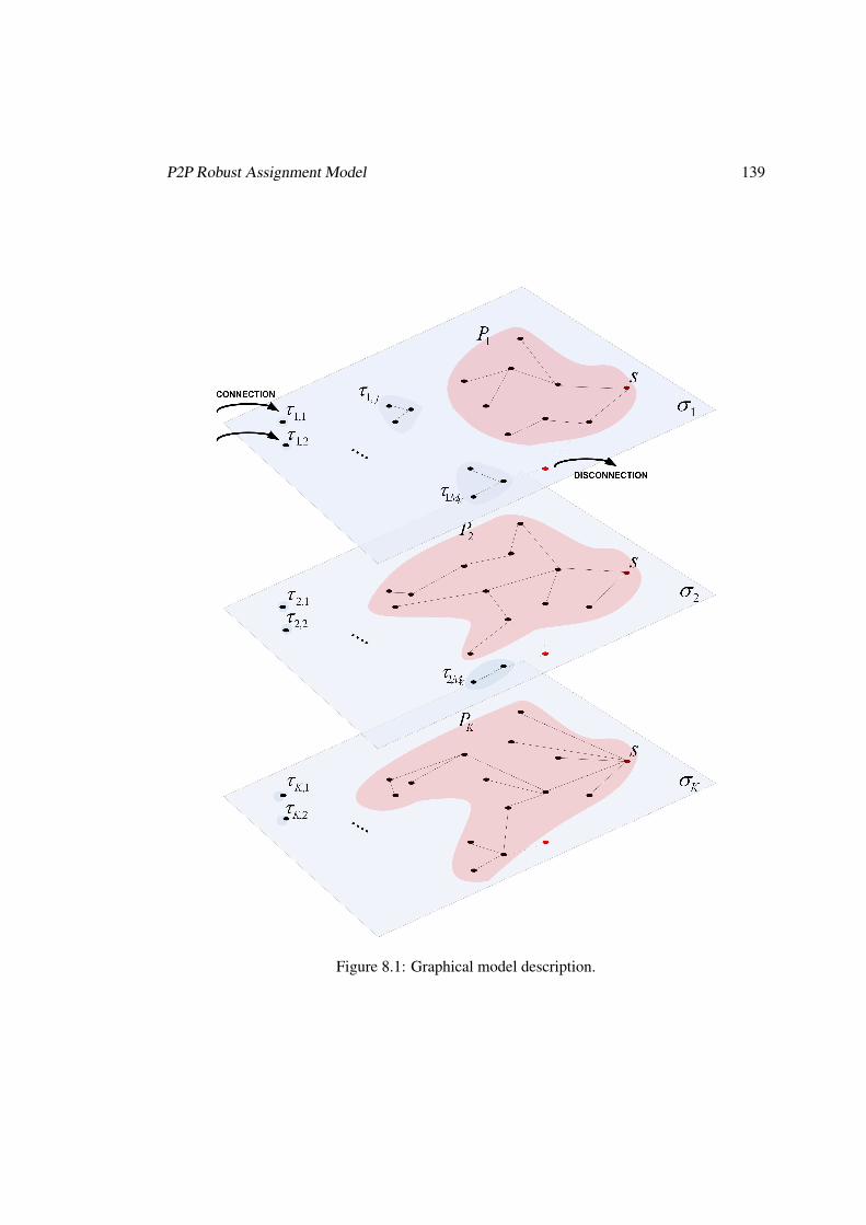
P2P Robust Assignment Model 139
Figure 8.1: Graphical model description.

140 Structured Overlay Peer-to-Peer based on Quality Guarantees
Since the perceived quality at node i depends on which substream is received by i, weassume available a function f() of K variables such that the quality at time tn experienced bynode i ∈ N (tn) (and measured using PSQA) is
Qi = f(y1s,i, y
2s,i, .., y
Ks,i).
For all i ∈ N (tn), let zi be the binary random variable defined at time tn by
zi =
{1 if node i will remain connected until (tn+1)−,0 otherwise,
where Pr(zi = 1) = pi.The sets
{xkij
}and
{ykij
}specify the network configuration at tn whereas the network
configuration at (tn+1)− is determined by the variables{xkij
}and
{ykij
}satisfying the fol-
lowing relations:
xki,j = zixki,jzj ,
yki,j = xki,j +N∑l=1
ziyki,lx
kl,j ,∀i ∈ N, ∀j ∈ N − {s},∀k ∈ K,
yki,j ≤ yki,j .
The PSQA evaluation of the quality as perceived by node i at time (tn+1)− is a random variablewhich is a function of
{yks,i
}and r.v. {zi}. We will maximize the expected value of the
perceived quality of all the nodes in the network. Actually, we use a scaled expression,
E
{∑Ni=1 Qi∑Ni=1 zi
}=
∑−→z ∈[0,1]N
∑Ni=1 Qi(−→z )∑Ni=1−→z i
p(z = −→z ),
where Qi = f(y1s,i, y
2s,i, .., y
Ks,i).
See Figure 8.2 for a summary of the complete model.
8.3 Looking for a Solution
The model developed in previous section is a stochastic, mixed integer non-linear programmingmodel, where the objective function is not given explicitly, but algorithmically (using the PSQAbuilt function for the QoE). It does not seem possible to explicitly solve it, even for small sizeproblems, while real-life applications require to take into account a large number of nodes. Ofcourse, in larger networks, it is possible to divide the nodes into small groups (for example,based on some proximity parameter), but this implies a separation from the global optimalnetwork. In some way, with the mathematical formalization we want to find the theoreticalefficiency bounds of a network with these characteristics, instead of analyzing its effectivedeployment.

Looking for a Solution 141
max E
(PNi=1 QiPNi=1 zi
)// global expected perceived quality
st:
yki,j + ykj,i ≤ 1, ∀i, j ∈ N, ∀k ∈ K, // loops are not allowed
yki,j = xki,j +
NXl=1
yki,lxkl,j , ∀i ∈ N,∀j ∈ N − {s}, ∀k ∈ K, // precedence constraints
NXi=1
xki,j ≤ 1, ∀j ∈ N, ∀k ∈ K, // each substream arrives from only one node
KXk=1
{bwkNXj=1
xki,j} ≤ BW out(i),∀i ∈ N, // bandwidth capacity constraints
xki,j = 1, ∀i ∈ N, ∀j ∈ N,∀k ∈ K|xki,j ∈ Ekt , // network configuration at t
xki,j = zixki,jzj , ∀i ∈ N, ∀j ∈ N,∀k ∈ K, // a link is preserved if source and terminal do not leave
yki,j = xki,j +
NXl=1
ziyki,lx
kl,j , ∀i ∈ N, ∀j ∈ N − {s}, ∀k ∈ K, // y represents the precedence at (tn+1)−
yki,j ≤ yki,j , ∀i ∈ N, ∀j ∈ N,∀k ∈ K,
zi ∼ Bern(pi), ∀i ∈ N, // random variables with Bernoulli distribution (parameters pi)
xki,j , yki,j ∈ {0, 1}, ∀i ∈ N,∀j ∈ N, ∀k ∈ K
Figure 8.2: Mathematical Programming Model.

142 Structured Overlay Peer-to-Peer based on Quality Guarantees
Instead of using exact solvers, we will look at some heuristics that can find feasible solu-tions, hopefully of good quality. In particular, we develop a greedy constructive heuristic, andtwo version of a GRASP-based metaheuristic.
As we have seen in the formal model description, the time line is divided into intervals ofthe form In = [tn, tn+1). In this way, we simplify the problem by considering only a discretenumber of points (t0, t1, t2, ...) on the time line. Just before each interval In (we will call thisinstant t−n ), the state of the network is the result of all the changes which have occurred in theprevious interval, In−1. During this period, some nodes may have left the network (willinglyor not), while new clients may have requested connection in order to receive the video stream.Therefore, new disconnected trees may have appeared. It is at this instant tn that our heuristicalgorithm is executed in order to connect the new nodes and disconnected trees to the maintree, and this has to be done in such a way that the expected quality is maximized, takinginto account the upstream bandwidth restrictions of each node. Theoretically, we assume aninstantaneous execution of the algorithm, so that at instant tn we will have our reconfiguredsystem1. Then, new connections and disconnections will occur during the interval In, and thealgorithm will be executed again at the beginning of In+1. The output of the algorithm will thenbe a set of assignments, where each assignment indicates to which node of the main tree wewill attach a disconnected tree (or a new node2) in order to enable the transmission of a certainsubstream to that tree. An assignment can then be seen as a triplet (parent, child, substream),where the child is the root of the disconnected tree which will be attached to a node of the maintree (the parent), in order to receive the corresponding substream. As it was stated before, thealgorithm should produce a solution which maximizes the global perceived quality, that is, asolution which satisfies the restriction of the formal model described before. However, we haveseen that this is an extremely difficult problem, so the algorithm will try to construct a solutionwhich is as close to the optimal one as possible.
8.3.1 Greedy heuristic solution
The Greedy algorithm constructs a solution based on a simple iterative decision process. Theprocedure used is outlined in Figure 8.3. The procedure GREEDYp2p is executed with theinitial state of the network g0. First, a list of all possible assignments is determined given thecurrent state of the network. That is, a list of all possible (parent, child, substream) tripletsis constructed to determine which trees need to be reconnected to the main one and whichnodes have enough upstream bandwidth available in order to transmit a certain substream toa disconnected tree (line 2). While an assignment will be possible, the procedure will chooseiteratively the “best” of them, until one of the two following conditions will be satisfied:
• all the disconnected trees have been reassigned to the main tree for each substream;
• no nodes in the main tree have enough bandwidth to transmit a substream to a discon-nected tree.
1In the actual implementation, this “instantaneous execution” would mean that the execution time of the algo-rithm has to be negligible compared to the duration of each interval In.
2New nodes can be seen as disconnected trees with only one element, so there is no need to make a distinction.

Looking for a Solution 143
Procedure GREEDYp2p
Input: g0
1: g ← g02: C ← FindAllAssignmentsCandidates(g)3: while C 6= ∅ do4: CPARENT ← SelectBestConnectedParent(g, C)5: CK ← SelectKLargestChilds(g, CPARENT )6: a← SelectBestCriteria(CK)8: C ← UpdateCandidates(g, a, C)9: g ← ApplyAssignments2Graph(g, {a})10: end while
11: return g
Figure 8.3: GREEDY algorithm
To choose the “best” assignment, we first select a subset of the set of all possible assignments(line 4). The assignments of this subset have the parents that provide the highest probabilityto be connected at the final of the current period. This is computed using the disconnectionprobability of each node in the path from the parent to the root. Then (line 5), from thissubset, we select one assignment per sub-stream (K in total). We choose the assignments thatconnect the largest number of nodes. If, at the same sub-stream, two assignments have the samenumber of nodes, we select the one that has the larger available bandwidth. Then, the candidateassignment that has the highest enhancement is chosen (line 6)3. The list of candidates is thenupdated (line 8). The assignment is applied to the graph (line 9), since the tree correspondingto the selected assignment will no longer be disconnected, and the upstream bandwidth of thenode to which that tree will be connected will have decreased. This process is repeated untilthere is no more possible assignments to do.
8.3.1.1 Enhancement criteria of a given assignment
Two different criteria are considered for estimating the enhancement provided by a certainassignment.
Current Perceived Quality. The “current” criterion selects the assignments which provide abetter perceived quality for the network at the current time.
Future Perceived Quality. The “future” criterion gives higher priority to the assignments thatwill result in better perceived quality for the next iteration. This is computed by a MonteCarlo estimation (by randomly simulating sequences of nodes entries and exits in theperiod). The precision and the time consumed by the estimation depend on the numberof simulations (trials).
3Three different criteria are considered for estimating the enhancement provided by a certain assignment (seebelow).

144 Structured Overlay Peer-to-Peer based on Quality Guarantees
Procedure GRASPp2p
Input: g0
1: q∗ ← −12: for i = 1 to imax do3: gi ← Constructionp2p(g0)4: qi ← PSQAexpected(gi)5: if (qi > q∗) then6: q∗ ← qi7: g∗ ← gi8: end if9: end for
10: return g∗
Procedure Constructionp2p
Input: g
1: C ← FindAllAssignmentsCandidates(g)2: A← ∅3: while C 6= ∅ do4: CRCL ← GenerateRCLp2p(g, C)5: a← SelectRandom(CRCL)6: A← A ∪ {a}7: C ← UpdateCandidates(g,A,C)8: end while9: gc ← ApplyAssignments2Graph(g,A)
10: return gc
Figure 8.4: GRASP-based algorithm
8.3.2 Algorithmic solution based on GRASP
GRASP [270] is a well known metaheuristic that has been successfully used to solve manyhard combinatorial optimization problems. It is an iterative process which operates in twophases. In the Construction Phase an initial feasible solution is built by means of a greedyalgorithm. This algorithm must also have a random component, so that different executionslead to different results. The neighborhood of this initial solution is then explored in the LocalSearch Phase, in order to improve locally the solution.
In the following sections, we describe the GRASP-based algorithm which is used to reas-sign connections in the network after a certain interval of time.
8.3.2.1 Construction phase
The objective of the Construction phase of the algorithm is to use a greedy and randomized pro-cedure to construct an initial solution for the problem. This solution can then be refined in theLocal Search phase. The procedure used for the Construction phase is outlined in Figure 8.4.
When the procedure GRASPp2p is executed with the initial state of the network g0, imaxinitial solutions are constructed (lines 1 - 3) using a procedure Constructionp2p. Since this pro-cedure has a random component, n executions of the procedure will lead to n different results.Then, from the imax solutions obtained, we pick the one which gives the network the betterglobal perceived quality in the future interval (lines 4 - 7). To evaluate the global perceivedquality in the future interval for each solution, we use the procedure PSQAexpected, which re-lies on statistical data about the nodes in order to “predict” the connections and disconnectionsin the future interval and see how a given solution is affected by these events. We will nowexamine the procedure used to construct each one of these initial solutions, Constructionp2p.First of all, a list of all possible assignments is determined given the current state of the network(line 1). Then, using a specific criterion, we select a subset of this set of all possible assign-ments (line 4) which is called Restricted Candidate List (RCL). The criterion used to selectthe “best” assignments is configurable4. Here we use the same enhancement criteria presented
4A specific interface in the algorithm must be implemented for each criterion.

Looking for a Solution 145
for the greedy algorithm, i.e. the current and future perceived quality. This subset will containthe assignments which provide the “better” quality improvement to our solution for the currentstate of the network according to the improvement criteria specified. This is the greedy part ofthe GRASP algorithm. Then, one of these candidate assignments is randomly selected fromthe RCL (line 5) and added to a set A (line 6), this constitutes the random component of thealgorithm. The list of candidates is then updated (line 7), since the tree corresponding to theselected assingment will no longer be disconnected, and the upstream bandwidth of the nodeto which that tree will be connected will have decreased. This process is repeated until the setA satisfies one of the two following conditions:
• All the disconnected trees have been reassigned to the main tree for each substream;
• No nodes in the main tree have enough bandwidth to transmit a substream to a discon-nected tree.
The set A of assignments is then our initial solution.
8.3.2.2 Local search phase
Our customized GRASP algorithm does not contain the traditional local search phase. In thelocal search phase, the solution built in the construction phase is improved by exploring itsneighborhood in order to find a local optimum. In the construction phase of our algorithm,a feasible solution is built applying successive individual assignments to the initial networkconfiguration. Let T = {a1, a2, ..., ak, ..., an} be the set of assignments applied to build afeasible solution. In this case, for the local search phase, the choice of the neighborhood struc-ture should be one where small variations on the assignments of T produce feasible solutions.The main problem here is that a particular assignment is strongly dependent on the previousone. In this sense, if we want to change assignment ak, there is a chance that next assignmentsak+1, ..., an could not be applied. This is easily seen when, for example, assignment ak+1
involves, as a parent, one of the new available parent nodes added in ak. That means that akmust not be changed in that particular case.
A local search phase is not useful in this specific problem, because it introduces a newcomplex combinatorial problem. Therefore, we will not implement this phase. Instead, wepropose an alternative way to improve the algorithm, based on the RNN model, of the solutionsbuilt during the GRASP construction phase. It consists on replacing the assignment selectionmethod in a random fashion, in order to explore new zones of the solution space, which mayallow us to find better solutions.
8.3.3 GRASP improvement using RNN
The Random Neural Network (RNN) model [101] has been applied with success to manydifferent optimization problems such as the minimun vertex covering problem [107] and thetraveling salesman problem [110]. In the RNN model, signals in the form of spikes of unitamplitude circulate among the neurons. Positive signals represent excitation, and negativesignals represent inhibition. Signals coming from the outside form Poisson processes. Thesemodels have been presented in Chapter 4 and used for learning purposes in deriving our PSQA

146 Structured Overlay Peer-to-Peer based on Quality Guarantees
modules (Chapter 5). Here, the main difference is in the neuron network topology, which, aswe will see, is arbitrary. The model is parameterized by the following elements: the number nof neurons, the firing rate ri of neuron i, the probability p+
ij (resp. p−ij), for a signal sent by i, togo to j as a positive (resp. negative) one, the probability di = 1−∑j(p
+ij + p−ij) of the signal
to go outside, and the exogenous rates αi and βi of the signal flows arriving at i. In the stablecase, probability qi that neuron i is excited, in steady state, is given by [101]
qi =λ+i
ri + λ−i
where λ+i and λ−i are defined as λ+
i =∑n
j=1 qjw+ji + αi, λ−i =
∑nj=1 qjw
−ji + βi, and the
weights are w+ji = rip
+ji, w
−ji = rip
−ji. Observe that the information contained in the RNN is
represented by the frequency at which the signals travel (the set of weights). The computationof the qi’s is thus a fixed point problem. See [101] for details about existence and unicity.During this computation, if we get a value qi > 1 then we force qi = 1 until convergence (wesay neuron i is saturated).
Following directly the ideas in [40], we use a RNN in the GRASP construction phase. Wereplace the RCL generation and the random assignment selection (lines 4-5 of Constructionp2p,Figure 8.4) with an RNN improved algorithm (explained below). In addition, on each construc-tion, a Bernoulli parameter, rnn, is used to determine which assignment selection is used: thisparameter indicates the probability of using the RNN based method for constructing solutionsin that iteration, instead of the original GRASP based method5.
Next, we present the algorithm based on the RNN model to solve the problem of selectingan specific assignment during the iterative process of the GRASP construction phase.
We define a neuron as the pair (node, substream), denoted by υk, which belongs to one ofthe following classes:
A = {υk | υ ∈ Pk , BW outv ≥ bwk ; k = 1, . . . ,K}
O = {υk | υ ∈ {τk,1, . . . , τk,Mk} , Mk ≥ 0 ; k = 1, . . . ,K}
We use Ak and Ok to denote the subsets of neurons of A and O respectively, where the nodesof the neurons are contained in the substream σk. In addition, we define a possible assignmentas the pair (i, j) where i ∈ Ak and j ∈ Ok, ∀k ∈ {1, . . . ,K}. The excitatory and inhibitoryweights of the neural network are set as follows:
w+ij =
AICij
AICi, if (i, j) is a possible assignment, (8.1)
w−ij = 1, otherwise, (8.2)
where AIC is the “assignment improvement criteria” function corresponding to the greedycriteria implemented in the same way it is done in GRASP. AICij is the evaluation of the AICfunction after the assignment (i, j) is applied and AICi is the average of all AIC functionevaluations corresponding to all possible assignments containing neuron i as a parent, which
5The algorithm GRASP+RNN with the parameter rnn = 0 is equivalent to the simple GRASP described before.

Looking for a Solution 147
Procedure Select_RNN_Assignmentp2p
Input: C, α, MaxIter
1: for each (i, j) ∈ C do2: compute w+
ij {using the equation 8.1}3: end for4: q = (q1, . . . , qn)← Initialize(n) {n-orphans neurons vector}5: compute F (q) {using the equation 8.3}6: while ||F (q)− q||2 > α and iter < MaxIter do7: q ← F (q)8: compute F (q) {using the equation 8.3}9: iter ← iter + 110: end while11: j∗ ← argmax
j{qj | j = 1, . . . , n}
12: i∗ ← argmaxi{AICi | (i, j∗) ∈ C} {AIC is the greedy function}
13: return (i∗, j∗)
Figure 8.5: RNN Algorithm
is formally defined as AICi =∑
j∈Ok AICij/∣∣Ok∣∣ where i ∈ Ak,∀k ∈ {1, . . . ,K}. All
other network parameters are set to zero. Using this set up, note that the firing rate is computedas ri =
∑j(w
+ij + w−ij). The connection weights have been chosen in a manner such that the
neural network captures connectivity information about the possible assignments which can bedone. When the neural network is set up in this manner, an excited neuron will have a greaterexcitatory effect on neurons which have high excitatory connections (i.e., higher assignmentimprovement) with it. Basically, the procedure in our RNN consists in artificially excitingthe parent neurons in A and then computing the values qj for all the orphan neurons in Oiteratively solving the fixed point problem using 8.3.3. According to the RNN set up presentedpreviously, we simplify Gelenbe’s equation as follows:
qj =
∑i qiw
+ij + αj
rj +∑
i qiw−ij + βj
=
∑i qiw
+ij∑
i(w+ji + w−ji) +
∑i qiw
−ij
=
∑i∈Ak w
+ij∑
iw−ji +
∑i∈Al∪O,l 6=k qi
=
∑i∈Ak w
+ij∑
iw−ji + (
∑p∈Al,l 6=k qp +
∑c∈O,c 6=j qc)
=
∑i∈Ak w
+ij
|A|+ |O| − 1 + (|A| − |Ak|+∑c∈O qc)
=
∑i∈Ak w
+ij
2|A| − |Ak|+ |O| − 1 +∑
c∈O,c 6=j qc, ∀j ∈ Ok with k = 1, . . . ,K. (8.3)
Figure 8.5 presents the pseudocode of the RNN algorithm. First, we compute the excitatoryweights for all the possible assignments (set C, candidates) (lines 1-3). This is necessary forthe computation of F (q) as can be seen in Equation 8.3 (line 5 and 8). Before the iteration,we need to initialize vector q (line 4); each neuron excitation probability is usually initializedwith a near zero value because this way, the network iterates until convergence in a smallernumber of steps. The stop criteria depends on the threshold α, and in case the iteration does

148 Structured Overlay Peer-to-Peer based on Quality Guarantees
not converge, we limit the number of iterations toMaxIter. When convergence is reached, wechoose the neuron j with the highest value qj (line 11) and then we compute the values AICifor all the neurons i ∈ A where (i, j) is a possible assignment. Finally, we choose the neuroni with the highest value AICi (line 12) and the assignment (i, j) is selected as the solution.
8.4 Preliminary performance estimation in a hybrid CDN-P2P struc-tured network
In the introduction to the background technologies (Section 2.3.4), we discussed the advan-tages of combining a Content Delivery Network (CDN) architecture with a Peer-to-Peer (P2P)network. The main idea was to extend the resources available in the CDN with the efficiencyof P2P delivery, keeping the high quality, security, and centralized control of the CDN.
In this section, we show how our tree-based overlay algorithms (presented in previoussection) performs in a hybrid architecture. When the data is available, we use real scenarioscoming from our video delivery reference service.
8.4.1 Generation of realistic test cases
We generate some instances from the collected real data of our reference service. A long traceof users connections/disconnections is used in order to specify the instances. Here, we willpresent five of these instances that come from a particular football match period. During thismatch, a server fails in the CDN, forcing the reconnection of many users over a short period.Studying this particular case allow us to analyze the behavior of our algorithm also during aflash crowd.
Each instance has a total duration of one hour. We consider a rebuilding period of tenseconds; therefore, there are a total of 360 iterations6 in each instance.
One instance has 30 simultaneous users on the average, while the other four instanceshave 60 simultaneous users on the average. Figure 8.6 shows the connection/disconnectiondynamics in the system (the four sixty users instances are tagged in the figure with differentK values, which be used later in the experiments). Usually, per iteration, between 0 and 1users change their state (connect/disconnet to/from the network), except at the 22th minute(130th iteration), when a server of the CDN fails, and disconnects a lot of peers (which will beimmediately reconnected to other server).
We choose the upload bandwidth capacity of the nodes sampling from an uniform distribu-tion between 256 Kbps and 1024 Kbps, because this information is not available in our refer-ence CDN service7. Figure 8.7(a) shows the obtained bandwidth distribution of each instance.The upload bandwidth available at the broadcaster (the root server) is 5 Mbps8. The total avail-able bandwidth in the peer-to-peer network changes with the peers connections/disconnections,
6The algorithms presented before have to be executed 360 times per instance.7Upload bandwidth bounds estimated from the popular http://broadbandreports.com speed-test, on
May, 2007.8Considering a streaming with bitrate 640 Kbps, only seven clients can be served simultaneously in a traditional
CDN architecture.

Preliminary performance estimation in a hybrid CDN-P2P structured network 149
0
10
20
30
40
50
60
70
80
0 50 100 150 200 250 300 350 400
user
s
iteration
User Connection/Disconnection Dynamics
N=30N=60,K=1N=60,K=2N=60,K=4
N=60,K=10
Figure 8.6: Evolution of the number of users connected in the system.
Figure 8.7(b) shows the evolution of the global available bandwidth (including the upload ca-pacity of each connected peer).
The probability to remain connected (Pr(zi = 1) = pi in our model) is obtained from sta-tistical information of each particular user included in the instances. For each user, we estimate,from his average lifetime behavior in several sessions, the probability to remain connected inthe next ten seconds. For this purpose, we use an exponential distribution9. Figure 8.8 showsthe distribution of the probability to remain connected in the next 10 seconds of each peer.
To deliver the video, we use four multi-source streaming configurations. We use the op-timal configurations specified in Table 7.12, for K ∈ {1, 2, 4, 10} (see Section 7.2 for detailsabout the procedure used to obtain these configurations). The bitrate of the original stream is512 Kbps, and a global redundancy of r = 25% is applied to achieve a overall bandwidth of640 Kbps (considering all the sub-streams). There is no constraint on the upload bandwidth ofthe multi-source streaming configurations chosen. Table 8.1 shows the bandwidth consumedper sub-stream for each configuration.
The perceived quality depends on which sub-stream is received by the user. The modeluses a function f() of K variables such that the quality at time tn experienced by node i isQi = f(y1
s,i, y2s,i, .., y
Ks,i). For instance, if K = 1, user i has perfect quality when he receives
the stream (Qi = f(1) = 10), and zero quality otherwise (Qi = f(0) = 0). We compute thequality function f() from the PSQA complex function of Section 5.3.3, using the loss processmodel described in Section 7.2. Tables 8.2 and 8.3 show the quality function f() for K = 2and K = 4 respectively. The quality function f() for the multi-source streaming with ten sub-streams (K = 10) is not shown here to save space. Observe that higher sub-streams indexeshave larger impact in the perceived quality (as we expect from the methodology presented inSection 7.2).
9This is for lack of enough data (observe that we consider here a specific client) and the choice means a priori apessimistic point of view.

150 Structured Overlay Peer-to-Peer based on Quality Guarantees
100
200
300
400
500
600
700
800
900
1000
1100
0 50 100 150 200 250
band
wid
th (
kbps
)
peer
Peer Upload Bandwidth
N=30N=60,K=1N=60,K=2N=60,K=4
N=60,K=10
(a) Upload bandwidth capabilities of the peers in the system.
5000
10000
15000
20000
25000
30000
35000
40000
45000
50000
0 50 100 150 200 250 300 350 400
band
wid
th (
kbps
)
iteration
Network Bandwidth Availability
N=30N=60,K=1N=60,K=2N=60,K=4
N=60,K=10
(b) Evolution of the global available bandwidth.
Figure 8.7: User bandwidth distributions.

Preliminary performance estimation in a hybrid CDN-P2P structured network 151
0.6
0.65
0.7
0.75
0.8
0.85
0.9
0.95
1
0 50 100 150 200 250
prob
abili
ty
peer
Peer Probability to Remain Connected
N=30N=60,K=1N=60,K=2N=60,K=4
N=60,K=10
Figure 8.8: Statistical probability distribution to peers’ remain connected in a given period(Pr(zi = 1) = pi).
Table 8.1: Upload bandwidth consumed on server i, for the multi-source streaming techniquedefined in Table 7.12, with K-substreams.
i/K 1 2 3 4 5
1 492.7 239.9 109.2 46.5 35.72 400.1 188.4 88.9 54.73 342.4 171.3 91.04 332.4 160.65 295.7
total 492.7 640.0 640.0 639.0 637.5
i/K 6 7 8 9 10
1 13.3 11.9 11.1 1.2 0.72 24.3 17.0 13.2 2.4 1.33 44.8 26.7 17.5 4.8 2.54 83.6 45.0 26.0 9.5 5.05 157.6 80.5 43.0 18.8 9.86 299.4 150.0 76.9 37.2 19.47 286.8 144.8 73.9 38.38 280.4 146.7 75.79 291.5 149.910 296.7
total 622.9 617.8 612.8 585.9 599.2
Table 8.2: Perceived quality function, Qi = f(y1s,i, y
2s,i), when K = 2. Values come from the
multi-source streaming technique defined in Table 7.12.
y1s,i y2s,i f()
0 0 0.000 1 3.641 0 2.281 1 10.00

152 Structured Overlay Peer-to-Peer based on Quality Guarantees
Table 8.3: Perceived quality function, Qi = f(y1s,i, y
2s,i, y
3s,i, y
4s,i), when K = 4. Values come
from the multi-source streaming technique defined in Table 7.12.
y1s,i y2s,i y3s,i y4s,i f()
0 0 0 0 0.000 0 0 1 2.310 0 1 0 1.400 0 1 1 4.820 1 0 0 1.040 1 0 1 3.450 1 1 0 2.090 1 1 1 7.701 0 0 0 0.901 0 0 1 2.881 0 1 0 1.751 0 1 1 6.171 1 0 0 1.281 1 0 1 4.361 1 1 0 2.661 1 1 1 10.00
Considering the four multi-source configurations, we generate four test cases from thesmall instance (N = 30). For each large instance (N = 60), we choose only one multi-sourceconfiguration. In what follows, we consider eight test cases, which will be denoted: N30K1,N30K2, N30K4, N30K10, N60K1, N60K2, N60K4, and N60K10.
8.4.2 Algorithms calibration
In order to test the implemented algorithms, we develop a program to simulate the behavior ofthe network during a certain period of time, divided into a discrete number of intervals. Thealgorithm to be executed at the end of each interval can be plugged into the simulator by imple-menting a specific function header. In our case, we implemented the Greedy heuristic, and theGRASP / GRASP+RNN based algorithms described in the previous sections10. This simulatorwas implemented in the C language, using the GNU C Compiler (gcc).
GRASP and GRASP+RNN are parametric in the size of the Restricted Candidate List(RCL), and GRASP+RNN also is parametric in the RNN use percentage (rnn). First, weneed to define suitable values for these parameters. We do this by evaluating the performanceof the algorithms with different parameter configurations, in the eight test cases.
The tests in this chapter were run on Intel Pentium 4 / AMD Athlon 64 machines with 1GB of RAM, running under Ubuntu Linux 6.10.
8.4.2.1 Restricted Candidate List (RCL)
For each test case, we execute the GRASP algorithm with three different RCL sizes. In par-ticular, we explore with the values RCL ∈ {5, 10, 25}.
10It is important to note that any assignment algorithm can be used provided its interface can be adapted to theone required by the algorithm.

Preliminary performance estimation in a hybrid CDN-P2P structured network 153
Also, we present the results for the two enhancement criteria of a given assignment pre-sented before, where “current” criteria selects the assignments which provide a better perceivedquality for the network at the current time; and the “future” criteria gives higher priority to theassignments that will result in better perceived quality for the next iteration. The “future”criteria is also parametric in the number of trials (we use 3, 5 and 10 trails).
We measure the global perceived quality (PSQA) of the network after running the assign-ment algorithm on each interval, as well as the execution time of the algorithm. Table 8.4shows the average perceived quality (our objective performance function) in each case. Theaverage is computed over all the iterations. The results do not show significant differencesbetween different RCL sizes. For this reason, we select RCL = 5, which leads to a moderatecomputational time.
Also, notice that the number of trails in the “future” criteria does not improve the solutionfor the considered values.
Table 8.4: GRASP performance for three different RCL sizes.
GRASPRCL = 5 RCL = 10 RCL = 25
test current future current future current futurecases 3 5 10 3 5 10 3 5 10
N30K1 4.44 4.02 4.18 4.15 4.42 4.37 4.19 4.39 3.61 4.30 4.33 4.05N30K2 7.29 7.31 7.48 7.16 7.19 7.53 7.69 7.54 7.02 7.01 6.35 7.38N30K4 9.51 8.97 8.86 9.57 9.72 9.17 9.29 9.68 9.79 9.35 9.51 9.44N30K10 10.00 10.00 9.99 9.71 10.00 9.99 10.00 9.99 10.00 10.00 9.95 10.00N60K1 3.64 3.31 3.04 3.13 3.82 3.45 3.62 3.64 3.30 3.55 3.51 3.75N60K2 6.48 5.18 5.32 5.77 5.82 5.47 5.64 5.81 6.20 6.10 6.04 4.76N60K4 5.24 5.09 6.61 5.42 6.03 5.25 6.14 6.06 5.88 5.55 6.03 5.71N60K10 10.00 9.51 9.64 9.68 10.00 9.83 9.82 9.77 9.92 9.76 9.44 9.75Average 7.08 6.67 6.89 6.82 7.12 6.88 7.05 7.11 6.96 6.95 6.90 6.85Average 6.8659 7.0415 6.9172
8.4.2.2 RNN use percentage (rnn) in the RNN-improved GRASP
In GRASP+RNN we need to define the percentual use of the RNN improvement (where rnn =1 means that all the assignments came from the improved selection, and rnn = 0 reduces theGRASP+RNN to the GRASP algorithm). We ran the simulation using several values for thernn parameter, rnn ∈ {0%, 25%, 50%, 75%, 100%}.
For instance, Figures 8.9(a) and 8.9(b) show the evolution of the PSQA during the simula-tion for each criteria in the N60K4 test case. As we can see, while the use of RNN initiallyleads to weaker results, this soon improves and then the perceived quality stabilizes at a higherlevel than the one obtained using GRASP-only assignments. We also observed, for the “future”improvement criteria, a noticeable decrease in the execution time of the algorithm when usingRNN (see Figure 8.9(c)).
Table 8.5 summarizes the GRASP+RNN global performance for the different rnn proba-bilities values. The use of high rnn values (rnn ≥ 0.75) degrades the algorithm performance.We select rnn = 0.25 for our GRASP+RNN algorithm.

154 Structured Overlay Peer-to-Peer based on Quality Guarantees
(a) PSQA evolution (“current” criteria)
(b) PSQA evolution (“future” criteria) (c) Execution time
Figure 8.9: Detail results for the N60K4 test case and the GRASP+RNN algorithm.
8.4.2.3 Selection of the enhancement criteria of a given assignment: “current” and “fu-ture” perceived quality
The three presented algorithms use a criteria to select the “best” assignment to be applied in theconstruction of the solution (see Section 8.3 for an introduction to the algorithms). The term“best” refers to how this assignment improves the current solution. Two criteria are evaluatedin our work: “current” and “future” perceived quality. Because of computation time costs, wemade our test of the “future” criteria with only three future possible scenarios (trails). Table 8.6shows the performance of the enhancement criteria for the studied algorithms. There are noimportant differences between the two criteria; we then choose the “future” criteria, expectingbetter performance (but higher execution times also) when we increase the number of trials.
Other possible criteria can be considered in future work. For instance, how to increase theavailable bandwidth with the assignment. It can be calculated as the addition of the availablebandwidth in the nodes of the disconnected tree. Intuitively, this favors solutions where moretrees can be added.
Preliminary performance estimation in a hybrid CDN-P2P structured network 155
Table 8.5: GRASP+RNN performance for four different rnn probabilities values.
GRASP+RNN (RCL = 5)rnn = 0.00 rnn = 0.25 rnn = 0.50 rnn = 0.75 rnn = 1.00
test current future current future current future current future current futurecases 3 3 3 3 3
N30K1 4.44 4.02 3.99 4.23 4.24 4.75 4.37 3.80 4.38 4.46N30K2 7.29 7.31 6.07 7.46 7.81 7.29 7.58 6.01 5.32 5.02N30K4 9.51 8.97 9.15 9.12 8.32 8.41 8.62 7.67 6.42 6.27N30K10 10.00 10.00 9.75 9.80 9.58 9.31 9.49 9.63 7.22 7.61N60K1 3.64 3.31 3.62 3.59 3.76 3.61 4.16 3.83 4.40 3.69N60K2 6.48 5.18 6.55 4.98 5.29 6.12 5.75 4.61 5.89 5.02N60K4 5.24 5.09 5.68 5.15 6.14 4.71 4.49 4.51 5.03 4.16N60K10 10.00 9.51 9.82 9.84 9.73 9.76 8.62 9.19 4.86 6.45Average 7.08 6.67 6.83 6.77 6.86 6.75 6.63 6.16 5.44 5.34Average 6.8747 6.7999 6.8016 6.3956 5.3875
Table 8.6: Performance of the enhancement criteria for the studied algorithms.
AlgorithmCriteria Greedy GRASP GRASP+RNN Average
(RCL = 5) (RCL = 5, rnn = 0.25)current 8.18 7.08 6.83 7.36future (3 trails) 8.00 6.67 6.77 7.15
8.4.3 Comparing the performance of our algorithms: Greedy, GRASP and GRASP+RNN
For each test case, Table 8.7 shows the global execution time, and the average perceived qualityconsidering all the iterations. The Greedy algorithm performs better than the GRASP-basedalgorithms, in terms of quality and execution time. The low performance of GRASP-basedalgorithms is related to the fact that they are tested with relative low parameter values (inparticular the number of GRASP iterations). Increasing the number of iterations in GRASPincrements linearly the computation time. With an average of 12 seconds (GRASP+RNN) inthe considered (small size) test cases, it can be considered only to estimate, in laboratory, theperformance of a constructive heuristic (like our Greedy proposal). In our GOL!P2P prototype(Chapter 10) we use the Greedy algorithm presented in this chapter.
Another observations can be extracted from the test results. For the two network sizestested (N = 30 and N = 60), with an increment of the number of sub-streams (K), the globalperformance of the method increases too. This is because of the relaxation of the problemconstraints with the K increment. It is possible to measure the number of nodes that receivethe stream with a low quality in each iteration. Table 8.8 shows the average percentage ofnodes that perceive a quality below 3 (poor). This is another measure of the improvement onthe solution with an increment in the number of sub-streams.
Moreover, the available bandwidth in the network is better used when K increases. Ta-ble 8.9 shows this behavior. This can also be used in order to increase the quality of the streamor its redundancy level, etc.

156 Structured Overlay Peer-to-Peer based on Quality Guarantees
Table 8.7: Average performance and Execution time of our three algorithms over all test cases.
AlgorithmGreedy GRASP GRASP+RNN
test (RCL = 5) (RCL = 5, rnn = 0.25)case PSQA Execution PSQA Execution PSQA Execution
time (sec) time (sec) time (sec)N30K1 5.89 0.0000 4.02 0.1602 4.23 0.0303N30K2 8.32 0.0028 7.31 0.5608 7.46 0.1984N30K4 9.44 0.0138 8.97 3.0304 9.12 1.1901N30K10 9.33 0.2099 10.00 22.6145 9.80 13.2700N60K1 6.28 0.0028 3.31 0.1354 3.59 0.1019N60K2 7.85 0.0221 5.18 4.2072 4.98 1.4518N60K4 7.57 0.1450 5.09 20.1412 5.15 7.0579N60K10 9.34 0.5635 9.51 101.9945 9.84 74.0193Average 8.00 0.1200 6.67 19.1055 6.77 12.1650
Table 8.8: Percentage of nodes that perceive with low quality.
AlgorithmGreedy GRASP GRASP+RNN
test (RCL = 5) (RCL = 5, rnn = 0.25)case %nodes %nodes %nodes
N30K1 0.44 0.65 0.62N30K2 0.22 0.31 0.32N30K4 0.08 0.14 0.12N30K10 0.00 0.00 0.00N60K1 0.40 0.72 0.69N60K2 0.22 0.62 0.65N60K4 0.33 0.67 0.66N60K10 0.00 0.00 0.00
8.4.4 Extending our Video Delivery Reference Service with a P2PTV system
We compare the performance of our P2P assignment metaheuristic with a traditional CDN-based implementation.
Two important variables have to be considered in the analysis: the global perceived qualityof the network, and the total bandwidth consumed (at the broadcaster and at the peers). We usethe N60K10 case, coming from our live video delivery service (see Section 2.5 for details).This service has 20.000 access of different users per month, and an average of 50 concurrentusers per live-TV channel.
In the CDN architecture case, the broadcaster is a set of servers in the ISP datacenter,where the bandwidth consumption is the most expensive component cost of the service. Thebroadcaster absorbs all the load of the clients, with a stream of 512 Kbps; this means at least50 Mbps of bandwidth in peak use. The broadcaster of the CDN does not fail11. If we considerthe packet losses in the network negligible, we can assume that the CDN network has a perfectglobal quality on the average (i.e Q = 10.00). We simulate a P2P architecture with the same
11Actually the servers in the CDN fails, but the load is absorbed immediately by another active server, and theusers do not perceive the failure.

Summary and Conclusions 157
Table 8.9: Percental global consumed bandwidth.
AlgorithmGreedy GRASP GRASP+RNN
test (RCL = 5) (RCL = 5, rnn = 0.25)case %BW %BW %BW
N30K1 0.622 0.612 0.629N30K2 0.837 0.801 0.723N30K4 0.997 0.997 0.997N30K10 0.997 0.997 0.931N60K1 0.678 0.654 0.670N60K2 0.894 0.447 0.425N60K4 0.997 0.997 0.997N60K10 0.997 0.997 0.925
clients’ behavior (connections/disconnections) than the real CDN. We split the original streamin four redundant sub-streams, with a total bandwidth consumption of 614 Kbps. Our resultsshow that the broadcaster absorbs only 5 Mbps, and the peers the rest of the load (in average0.6 Mbps per peer). The quality is not considerably degraded, with a worst case of Q = 9.34on the average.
The numerical results obtained show the interest of employing a live-video P2P distributionsystem following a multi-source procedure.
8.5 Summary and Conclusions
In this chapter we present a preliminary design of a centralized tree-based overlay topology,for our P2PTV system.
The overlay is built choosing which peer will serve which other one. The assignment hasto be done in a way to diminish the impact of peers disconnection on the quality. We model theoverlay building as a mathematical programming problem, where the optimization objective isto maximize the global expected QoE of the network, calculated using the PSQA methodology.We present three algorithms for solving this problem, applied to cases study based on real lifedata.
This is just a first study that shows the possibilities of our approach. Future work is neededto improve the assignment algorithm. For instance, considering other enhancement criteria(like the available bandwidth), or using the presented greedy algorithm inside the GRASP.Finally, larger test cases have to be analyzed.

158 Structured Overlay Peer-to-Peer based on Quality Guarantees

Part IV
CHALLENGES IN THE REALITY
159


Chapter 9
Measure and Monitor the Quality ofReal Video Services.
Different network architectures are developed to deliver video transparently to end users. Inour work we grouped these architectures under the name Video Delivery Networks (VDNs)(VDNs are presented in Section 2.2).
This chapter presents a full Video Delivery Network (VDN) monitoring suite. Our moni-toring tool offers a new view of a VDN, a view based on the quality perceived by final users.We measure, in real time and automatically, the perceived quality at the client side by meansof the PSQA methodology (see Chapters 4 and 5).
The developed monitoring suite is a completely free-software application, based on well-known technologies such as the Simple Network Management Protocol (SNMP) or the RoundRobin Databases (RRD Tool), which can be executed in various operating systems. It is anextensible measurement framework that can be applied to most of the studied VDNs.
In this chapter we explain the tool implementation and we present some of the first ex-perimental measurements performed with it. This work has been partially presented at the7th IEEE International Workshop on IP Operations and Management (IPOM’07) [331] (listedat the Introduction as [ipom07audit]). The implementation of the suite has been completedwith the contribution of J.L. Fernandez, D. De Vera and A. Chadarevian, who completed theirengineering project at the Universidad de la República, Uruguay, in this subject.
9.1 Introduction
Video delivery systems may have many different architectures, each one with different points offailure and key components. For each architecture, monitoring and measurement are necessaryin order to get a satisfactory Quality of Experience level with a minimal cost. To identify factorsplaying an important role on QoE, some specific quantitative aspects must be considered [87](see also our discussion about this topic in Subsection 2.2.2). For video delivery services, themost important one is the perceptual video quality measure. Accurate video-quality measure-ment and monitoring is today an important requirement of industry. Service providers need tomonitor the performance of various network layers and service layer elements, including those
161
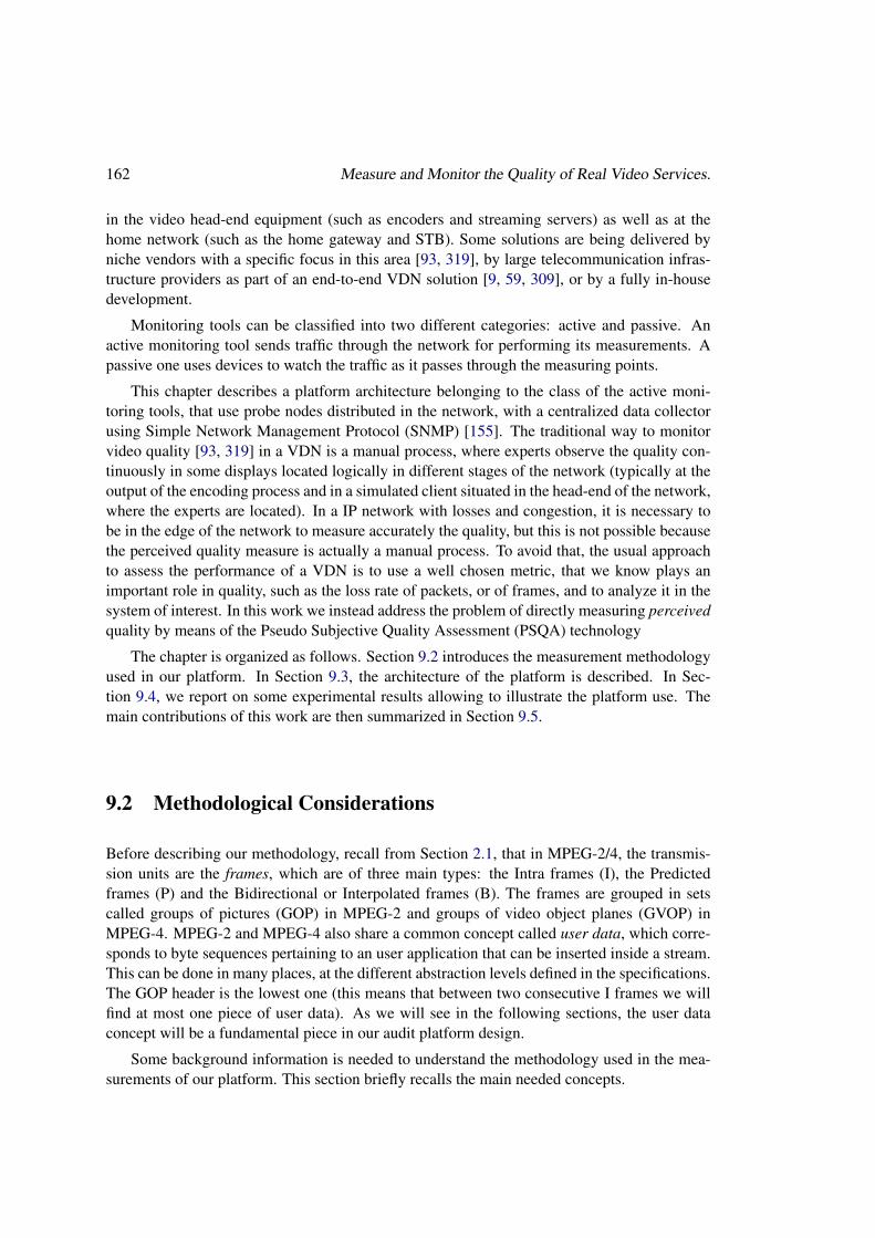
162 Measure and Monitor the Quality of Real Video Services.
in the video head-end equipment (such as encoders and streaming servers) as well as at thehome network (such as the home gateway and STB). Some solutions are being delivered byniche vendors with a specific focus in this area [93, 319], by large telecommunication infras-tructure providers as part of an end-to-end VDN solution [9, 59, 309], or by a fully in-housedevelopment.
Monitoring tools can be classified into two different categories: active and passive. Anactive monitoring tool sends traffic through the network for performing its measurements. Apassive one uses devices to watch the traffic as it passes through the measuring points.
This chapter describes a platform architecture belonging to the class of the active moni-toring tools, that use probe nodes distributed in the network, with a centralized data collectorusing Simple Network Management Protocol (SNMP) [155]. The traditional way to monitorvideo quality [93, 319] in a VDN is a manual process, where experts observe the quality con-tinuously in some displays located logically in different stages of the network (typically at theoutput of the encoding process and in a simulated client situated in the head-end of the network,where the experts are located). In a IP network with losses and congestion, it is necessary tobe in the edge of the network to measure accurately the quality, but this is not possible becausethe perceived quality measure is actually a manual process. To avoid that, the usual approachto assess the performance of a VDN is to use a well chosen metric, that we know plays animportant role in quality, such as the loss rate of packets, or of frames, and to analyze it in thesystem of interest. In this work we instead address the problem of directly measuring perceivedquality by means of the Pseudo Subjective Quality Assessment (PSQA) technology
The chapter is organized as follows. Section 9.2 introduces the measurement methodologyused in our platform. In Section 9.3, the architecture of the platform is described. In Sec-tion 9.4, we report on some experimental results allowing to illustrate the platform use. Themain contributions of this work are then summarized in Section 9.5.
9.2 Methodological Considerations
Before describing our methodology, recall from Section 2.1, that in MPEG-2/4, the transmis-sion units are the frames, which are of three main types: the Intra frames (I), the Predictedframes (P) and the Bidirectional or Interpolated frames (B). The frames are grouped in setscalled groups of pictures (GOP) in MPEG-2 and groups of video object planes (GVOP) inMPEG-4. MPEG-2 and MPEG-4 also share a common concept called user data, which corre-sponds to byte sequences pertaining to an user application that can be inserted inside a stream.This can be done in many places, at the different abstraction levels defined in the specifications.The GOP header is the lowest one (this means that between two consecutive I frames we willfind at most one piece of user data). As we will see in the following sections, the user dataconcept will be a fundamental piece in our audit platform design.
Some background information is needed to understand the methodology used in the mea-surements of our platform. This section briefly recalls the main needed concepts.

Methodological Considerations 163
9.2.1 Simple Network Management Protocol
Simple Network Management Protocol (SNMP) [155] is a widely diffused protocol used tomanage different resources and applications within a network. Network management systemscontain two primary elements: the manager itself and the agents. The manager is the consolethrough which the network administrator performs network management functions. Agents arethe entities that interface to the actual device or application being managed. In the agent thereshould be one or more objects (parameters) to monitor. These objects should be defined on amanagement information base (MIB). The manager can read and/or modify the objects definedinside the MIB, carrying out this way the administration of each one of these objects.
SNMP has been used in previous situations for network monitoring by means of probes [152]1,with an integrated logging module [151], a scenario very similar to ours. Our applicationuses the SNMPv3 [155, 157] version and our designed MIB module is compliant with theSMIv2 [147, 149, 150].
9.2.2 Quality Measurements.
We want to measure the video quality in real–time, in particular the quality perceived by endusers. As we know, traditional video quality assessments do not match well with this require-ment. Subjective tests are very time-consuming and expensive in manpower, which makesthem hard to repeat often. By definition, they cannot be a part of an automatic process. Theother approach, called objective metrics, often provide assessments that do not correlate wellwith human perception, and thus their use as a replacement of subjective tests is limited. Fur-thermore, with a few exceptions, objective metrics needs the received and the original videosequences to compute the metric, so, it is not possible to use them in a real–time monitoringenvironment. A survey of traditional video quality assessments is presented in Chapter 3.
Here, we exploit the advantages of the Pseudo Subjective Quality Assessment (PSQA)hybrid approach explained in Chapter 4. PSQA gives us a mapping function from some quality-affecting parameters into the perceived quality. It is very easy to use in a monitoring suite: weneed to measure the values of the chosen parameters at time t, and then to put them into thePSQA function Q() to obtain an estimation of the instantaneous perceived quality at t.
Depending on the Video Delivery Network, our prototype can be adapted to different pa-rameters, including network and application level parameters. In our tests, we use the PSQAsimple function presented on Section 5.2.3.
9.2.3 An Extensible Measurement Framework.
We distinguish two main components within our measuring system: a set of probes (actually,video players) and a family of centralized monitoring servers (usually the service itself). Thevideo players are an improved version of the VideoLan client software (VLC) [334]. Each VLCclient performs the measuring tasks, and makes the measures available to the servers using theSimple Network Management Protocol (SNMP) [155]. A collector server polls the clients toobtain the SNMP MIB values of the measured parameters.
1Probes are remote network monitoring devices useful for the network management.
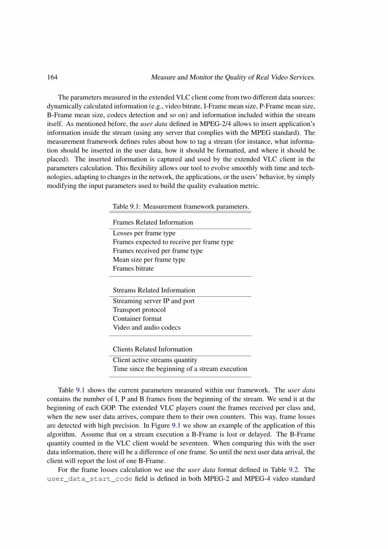
164 Measure and Monitor the Quality of Real Video Services.
The parameters measured in the extended VLC client come from two different data sources:dynamically calculated information (e.g., video bitrate, I-Frame mean size, P-Frame mean size,B-Frame mean size, codecs detection and so on) and information included within the streamitself. As mentioned before, the user data defined in MPEG-2/4 allows to insert application’sinformation inside the stream (using any server that complies with the MPEG standard). Themeasurement framework defines rules about how to tag a stream (for instance, what informa-tion should be inserted in the user data, how it should be formatted, and where it should beplaced). The inserted information is captured and used by the extended VLC client in theparameters calculation. This flexibility allows our tool to evolve smoothly with time and tech-nologies, adapting to changes in the network, the applications, or the users’ behavior, by simplymodifying the input parameters used to build the quality evaluation metric.
Table 9.1: Measurement framework parameters.
Frames Related InformationLosses per frame typeFrames expected to receive per frame typeFrames received per frame typeMean size per frame typeFrames bitrate
Streams Related InformationStreaming server IP and portTransport protocolContainer formatVideo and audio codecs
Clients Related InformationClient active streams quantityTime since the beginning of a stream execution
Table 9.1 shows the current parameters measured within our framework. The user datacontains the number of I, P and B frames from the beginning of the stream. We send it at thebeginning of each GOP. The extended VLC players count the frames received per class and,when the new user data arrives, compare them to their own counters. This way, frame lossesare detected with high precision. In Figure 9.1 we show an example of the application of thisalgorithm. Assume that on a stream execution a B-Frame is lost or delayed. The B-Framequantity counted in the VLC client would be seventeen. When comparing this with the userdata information, there will be a difference of one frame. So until the next user data arrival, theclient will report the lost of one B-Frame.
For the frame losses calculation we use the user data format defined in Table 9.2. Theuser_data_start_code field is defined in both MPEG-2 and MPEG-4 video standard
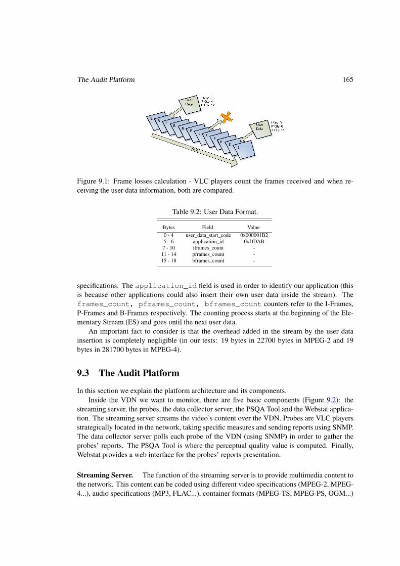
The Audit Platform 165
Figure 9.1: Frame losses calculation - VLC players count the frames received and when re-ceiving the user data information, both are compared.
Table 9.2: User Data Format.
Bytes Field Value0 - 4 user_data_start_code 0x000001B25 - 6 application_id 0xDDAB
7 - 10 iframes_count -11 - 14 pframes_count -15 - 18 bframes_count -
specifications. The application_id field is used in order to identify our application (thisis because other applications could also insert their own user data inside the stream). Theframes_count, pframes_count, bframes_count counters refer to the I-Frames,P-Frames and B-Frames respectively. The counting process starts at the beginning of the Ele-mentary Stream (ES) and goes until the next user data.
An important fact to consider is that the overhead added in the stream by the user datainsertion is completely negligible (in our tests: 19 bytes in 22700 bytes in MPEG-2 and 19bytes in 281700 bytes in MPEG-4).
9.3 The Audit Platform
In this section we explain the platform architecture and its components.Inside the VDN we want to monitor, there are five basic components (Figure 9.2): the
streaming server, the probes, the data collector server, the PSQA Tool and the Webstat applica-tion. The streaming server streams the video’s content over the VDN. Probes are VLC playersstrategically located in the network, taking specific measures and sending reports using SNMP.The data collector server polls each probe of the VDN (using SNMP) in order to gather theprobes’ reports. The PSQA Tool is where the perceptual quality value is computed. Finally,Webstat provides a web interface for the probes’ reports presentation.
Streaming Server. The function of the streaming server is to provide multimedia content tothe network. This content can be coded using different video specifications (MPEG-2, MPEG-4...), audio specifications (MP3, FLAC...), container formats (MPEG-TS, MPEG-PS, OGM...)
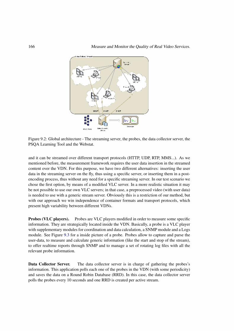
166 Measure and Monitor the Quality of Real Video Services.
Figure 9.2: Global architecture - The streaming server, the probes, the data collector server, thePSQA Learning Tool and the Webstat.
and it can be streamed over different transport protocols (HTTP, UDP, RTP, MMS...). As wementioned before, the measurement framework requires the user data insertion in the streamedcontent over the VDN. For this purpose, we have two different alternatives: inserting the userdata in the streaming server on the fly, thus using a specific server, or inserting them in a post-encoding process, thus without any need for a specific streaming server. In our test scenario wechose the first option, by means of a modified VLC server. In a more realistic situation it maybe not possible to use our own VLC servers; in that case, a preprocessed video (with user data)is needed to use with a generic stream server. Obviously this is a restriction of our method, butwith our approach we win independence of container formats and transport protocols, whichpresent high variability between different VDNs.
Probes (VLC players). Probes are VLC players modified in order to measure some specificinformation. They are strategically located inside the VDN. Basically, a probe is a VLC playerwith supplementary modules for coordination and data calculation, a SNMP module and a Logsmodule. See Figure 9.3 for a inside picture of a probe. Probes allow to capture and parse theuser-data, to measure and calculate generic information (like the start and stop of the stream),to offer realtime reports through SNMP and to manage a set of rotating log files with all therelevant probe information.
Data Collector Server. The data collector server is in charge of gathering the probes’sinformation. This application polls each one of the probes in the VDN (with some periodicity)and saves the data on a Round Robin Database (RRD). In this case, the data collector serverpolls the probes every 10 seconds and one RRD is created per active stream.

The Audit Platform 167
Figure 9.3: VLC Probe - A probe is a VLC player with the aggregate of the coordination anddata calculation module, SNMP module and Logs module.
PSQA Tool. The PSQA Tool receives the quality–affecting parameters from the probes andcomputes the perceived quality of each one. In operation, the use of PSQA is very simple: theprobes send statistical information about the quality–affecting parameters in a short period tothe data collector, to be evaluated by the PSQA Tool. The period size can be arbitrarily definedfor the specific application, and it is usually recommended to make it quite short, in order touse PSQA as an instantaneous quality value.
Webstat. Webstat is an application designed to present the data gathered by the data collec-tor server to administrators and managers of the VDN. It offers reports at different levels andtypes of views. It is possible to generate reports focused on a particular stream or on a specificclient (where there could be more than one active stream), or perhaps on the entire network(where there could be more than one client). Finally, it is possible to display the results at theframe level, possibly per frame type (I, P, B), or at the PSQA level.
Implementation. As mentioned before, both the probes and the streaming server are basedon a VLC Player. The libavcodec (ffmpeg) library was used in order to work withMPEG-2 and MPEG-4 video specifications. As container format we worked with MPEG-TSusing the functionalities provided by libdvbps. We streamed over HTTP and UDP usingVLC internal modules. In order to report the probes’s measures through SNMP we used theNet-SNMP library. We used the RRDtool to generate the statistical graphs. The data collec-tor server was written in PHP and we used the following PHP extensions: php4-snmp andphp4-rrdtool. Webstat is also written in PHP; it uses MySQL as relational database andit runs over Apache. All libraries and applications mentioned above are free-software and theycan be executed in Microsoft Windows, Unix, Linux, etc.
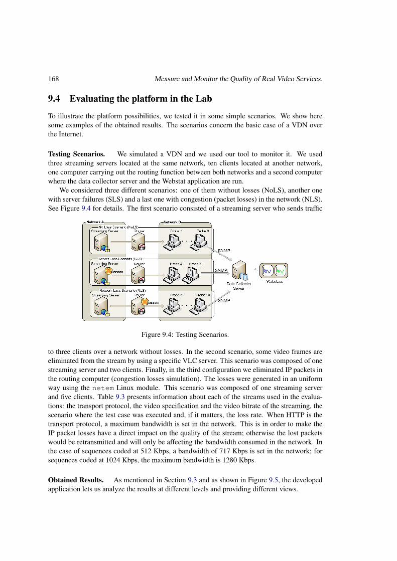
168 Measure and Monitor the Quality of Real Video Services.
9.4 Evaluating the platform in the Lab
To illustrate the platform possibilities, we tested it in some simple scenarios. We show heresome examples of the obtained results. The scenarios concern the basic case of a VDN overthe Internet.
Testing Scenarios. We simulated a VDN and we used our tool to monitor it. We usedthree streaming servers located at the same network, ten clients located at another network,one computer carrying out the routing function between both networks and a second computerwhere the data collector server and the Webstat application are run.
We considered three different scenarios: one of them without losses (NoLS), another onewith server failures (SLS) and a last one with congestion (packet losses) in the network (NLS).See Figure 9.4 for details. The first scenario consisted of a streaming server who sends traffic
Figure 9.4: Testing Scenarios.
to three clients over a network without losses. In the second scenario, some video frames areeliminated from the stream by using a specific VLC server. This scenario was composed of onestreaming server and two clients. Finally, in the third configuration we eliminated IP packets inthe routing computer (congestion losses simulation). The losses were generated in an uniformway using the netem Linux module. This scenario was composed of one streaming serverand five clients. Table 9.3 presents information about each of the streams used in the evalua-tions: the transport protocol, the video specification and the video bitrate of the streaming, thescenario where the test case was executed and, if it matters, the loss rate. When HTTP is thetransport protocol, a maximum bandwidth is set in the network. This is in order to make theIP packet losses have a direct impact on the quality of the stream; otherwise the lost packetswould be retransmitted and will only be affecting the bandwidth consumed in the network. Inthe case of sequences coded at 512 Kbps, a bandwidth of 717 Kbps is set in the network; forsequences coded at 1024 Kbps, the maximum bandwidth is 1280 Kbps.
Obtained Results. As mentioned in Section 9.3 and as shown in Figure 9.5, the developedapplication lets us analyze the results at different levels and providing different views.

Evaluating the platform in the Lab 169
Table 9.3: Scenarios Configuration. Each test case correspond to a client receiving a stream.Each scenario correspond to a failure situation: without losses (NoLS), with server failures(SLS) and with packet losses in the network (NLS).
Test Case Protocol Video Specification Video Bitrate (Kbps) Scenario Loss Rate1 UDP MPEG-2 1024 NoLS -2 HTTP MPEG-2 1024 NoLS -3 HTTP MPEG-4 512 NoLS -4 HTTP MPEG-4 512 SLS 0.505 HTTP MPEG-4 1024 SLS 0.306 UDP MPEG-2 512 NLS 0.307 UDP MPEG-2 1024 NLS 0.308 UDP MPEG-4 1024 NLS 0.309 HTTP MPEG-2 1024 NLS 0.02
10 HTTP MPEG-4 1024 NLS 0.04
Figure 9.5(a) shows a global view of the relative error measured during the evaluation atthe frame level. This information can also be provided on a per-frame type basis (I-Frame,P-Frame, B-Frame).
Figure 9.5(b) shows the evolution of global quality (PSQA) with time, normalized to num-bers in the interval [0, 1]. We use the PSQA simple function presented on Section 5.2.3, thatmapping LR and MLBS into perceived quality. Table 9.4 presents some values obtained when
Table 9.4: Obtained Results.
Test Case Protocol Specified Loss Rate Measured Frame Loss Rate Mean PSQA1 UDP - - 10.02 HTTP - - 10.03 HTTP - - 10.04 HTTP 0.50 (Frame level) 0.47 4.25 HTTP 0.30 (Frame level) 0.29 6.16 UDP 0.30 (IP level) 0.09 7.97 UDP 0.30 (IP level) 0.19 6.68 UDP 0.30 (IP level) 0.33 3.89 HTTP 0.02 (IP level) 0.08 7.9
10 HTTP 0.04 (IP level) 0.07 8.9
executing the simulations. As it can be observed, there is no visible relationship between IPpacket losses and frame losses. This is because this relationship depends on various factors:the video specification, the video bitrate, and the specific player software that processes thestream. However, there is a clear relationship between the loss rate and the PSQA value: thehigher the loss rate the lower the quality perceived by the users.
Last, Figure 9.6(a) shows the frame losses measured during a test case where server failuresoccur and Figure 9.6(b) shows the frame losses measured during a test case with network losses.
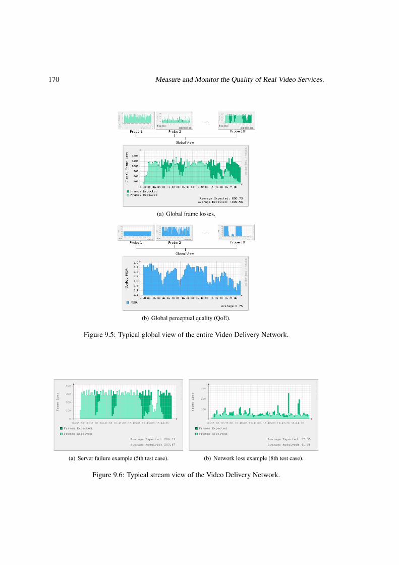
170 Measure and Monitor the Quality of Real Video Services.
(a) Global frame losses.
(b) Global perceptual quality (QoE).
Figure 9.5: Typical global view of the entire Video Delivery Network.
16:38:00 16:39:00 16:40:00 16:41:00 16:42:00 16:43:00 16:44:00
0
100
200
300
400
Frame Loss
RRDTOOL / TOBI OETIKER
Frames Expected
Frames Received
Average Expected: 284.19
Average Received: 203.67
(a) Server failure example (5th test case).
16:38:00 16:39:00 16:40:00 16:41:00 16:42:00 16:43:00 16:44:00
100
200
300
Frame Loss
RRDTOOL / TOBI OETIKER
Frames Expected
Frames Received
Average Expected: 62.35
Average Received: 41.38
(b) Network loss example (8th test case).
Figure 9.6: Typical stream view of the Video Delivery Network.

Summary and Conclusions 171
9.5 Summary and Conclusions
This chapter presents an effective monitoring and measuring tool that can be used by VDNmanagers and administrators to assess the streaming quality inside the network. With this toolit is possible to automatically monitor different sets of parameters of the streams, in real-timeif necessary, including the perceived quality as seen by the final users, thanks to our improvedversion of the recently proposed PSQA technology. PSQA provides an accurate approximationof the QoE (Quality of Experience) and, to the best of our knowledge, our tool is the onlyone that is able to evaluate perceived quality continuously at arbitrarily chosen points in thenetwork.
Another important feature of the presented suite is that it is not dependent on the consideredVDN. It was designed as a generic implementation, in order to be able to use it with differentVDN architectures. Moreover, it can be associated with most common management systemssince it is built over the SNMP standard. Another feature is that the induced overhead is negli-gible. Finally, the tool is a free-software application that can be executed on several operatingsystems.

172 Measure and Monitor the Quality of Real Video Services.

Chapter 10
GOL!P2P: A P2P Prototype forRobust Delivery High Quality LiveVideo
In this chapter we present our GOL!P2P prototype for live video streaming using a P2P net-work. Section 10.1 explains the core delivery system, i.e. the multi-source streaming imple-mentation. This section has been partially presented at the 7th IEEE International Workshop onIP Operations and Management (IPOM’07) [285] (listed at the Introduction as [ipom07msource]).The implementation of the tool was made possible by the work of L. Stábile, who completed hisengineering project at the Universidad de la República, Uruguay, in this subject. Section 10.2presents the global architecture and main components of our prototype. In Section 10.3 wereport on some integrated experimental results which illustrate the system performance in areal situation. The global prototype and the tests have been submitted [284] (listed at the Intro-duction as [submitted08a]). The chapter finalizes with general conclusions (Section 10.4).
10.1 Generic Multi-source Streaming Implementation
We will focus on the case of a P2P architecture where the video flow is decomposed into piecesand sent through the network. Each node receives the flow from different sources and buildsthe original stream before it is played. At the same time, it will, in general, send each of thesubstreams to a different client, acting then as a server. At the beginning, the (single) initialstream is split into several substreams, according to some specific scheme. With these goals,we need the two basic following services: (i) a flexible “splitter” where the original stream isdecomposed into different substreams, and (ii) a module capable of reconstructing the originalstream from the set of substreams, or a degraded version of it if some of the substreams hadlosses, or is simply missing. Associated with these services we want to design a very flexibletransport scheme, allowing to transport the original information plus some redundancy, withhigh control on which server sends which part of the flow and of the redundant information(see below).
Let us now briefly describe these different components of the project. The splitter must
173

174 GOL!P2P: A P2P Prototype for Robust Delivery High Quality Live Video
be able to obey a general scheme where we decide how many substreams are to be used, andwhich of the frames are to be sent through which of the substreams. This generality allows usto send, for instance, most of the frames through the highest performing nodes in the network,or to balance the load among the different components, or to adopt a scheme where the typeof frame is used to take the routing decision. It must also be possible to send an extra fractionr of the original stream, or of a specific population of the frames (for instance, the I frames)again according to any pre-specified scheme. If r = 0 there is no redundancy at all. If r = 0.2we send 20% of supplementary redundant data, and r = 1 means that the original stream isactually sent twice to the receiver(s). We do not consider r > 1 because, in a real system,this would mean too much bandwidth consumption. At the client side, we must be able toreconstruct the original stream if we receive all the frames, but also if only a part of the streamarrives; this typically happens when some of the servers fails (that is, they disconnect from theP2P network).
We extend the VLC software to send and to receive video streaming from multiple sources.The multi-source streaming technique implemented is the most general one; for instance, theimproved optimal version explained in Section 7.2 can be configured. In this section, wedescribe the method together with the design decisions and the operation characteristics ofthe tool. We illustrate the behavior of the tool by means of some tests.
10.1.1 Implementation Design
There areK servers and each server is identified by an index between 1 andK. The implemen-tation consists of three VLC modules, one at the server side and two at the client side. They arecalled msource-server, msource-bridge and msource-client (see Figure 10.1).
Figure 10.1: Architecture multiple-source in VLC

Generic Multi-source Streaming Implementation 175
The module msource-server, located at the server, decides which frames are to be sentto the client. It builds a substream for audio and another one for video. The basic constraintto satisfy is, of course, that each frame in the original stream must be sent at least once by oneof the servers. Once the frames selected by msource-server, the module standard ofVLC sends them to the client.
At the client’s side, there are K modules msource-bridge, one per server and eachwith its own buffer. The kth one receives the frames sent by server k. The last module,msource-client, receives the flows sent by the K modules msource-bridge and re-constructs the stream. This task consists of ordering the frames according to their decoding time(called DTS). The output of a module msource-client can be stored on the local disk, sentsomewhere through the network (both tasks are performed by the module standard, whichis a part of the VLC package) or played by the client.
The ideal case is when all the servers start their transmissions simultaneously and keepsynchronized, but this never happens in practice. It means that the system must handle the pos-sible shift between the servers. Moreover, since we don’t assume that the servers are identical,we implement a strategy allowing to control the bandwidth used by each of them. Observe thatthese modules work at the frame level in the flow; it implies that our multi-source implemen-tation is general and can be used with several video codecs, container formats and transportprotocols. No extra signaling is used in the method.
10.1.1.1 Basic Server Algorithm
The strategy used by the servers allows to control the bandwidth used by each of them, forinstance, to be able to send more information through the most reliable one, or through theone having the best performance. This control is implemented by acting on the percentage offrames of each type that the server must send. We must decide which fraction p(c)
k of the class cframes, c ∈ {I, P, B, A} 1 is going to be sent through server k. We must then have
K∑k=1
p(c)k = 1, c ∈ {I, P, B, A}. (10.1)
The sending algorithm works as follows. All the servers run the same pseudo-random numbergenerator and build a sequence of pseudo-random real numbers uniformly distributed on [0, 1].Not only they run the same generator but they use the same seed. In this way, they obtain thesame sequence of real numbers (u1, u2, · · · ) behaving as a realization of the correspondingsequence of i.i.d. random variables uniformly distributed on [0, 1].
Now, look at (p(c)k )k=1,··· ,K , for fixed c, as a probability distribution, and call X(c) the
corresponding random variable. It can be sampled from an uniform random variable U usingthe classical algorithm given by
X(c) = k ⇐⇒ P(c)k−1 ≤ U < P
(c)k , (10.2)
where P (c)j = p
(c)1 + · · ·+ p
(c)j , j = 1, · · · ,K, and P (c)
0 = 0.
1In MPEG, basically there are three classes of video frames (I, P and B), and one class of audio frames (A).

176 GOL!P2P: A P2P Prototype for Robust Delivery High Quality Live Video
Now, let fn be the nth frame of the stream, n ≥ 1, and let cn ∈ {I, P, B, A} be the classof fn. Any of the K servers will then run the same algorithm. They all sample the randomvariableX(c), and obtain the same value sn, with 1 ≤ sn ≤ K. That is, they all look at the typeof fn, and use (10.2). Server sn sends fn and the remaining servers don’t. This constructionguarantees that one and only one server sends each frame, and since sn behaves as a realizationof random variableX(c), after sending many frames the fraction of type c frames sent by serverk will be close to p(c)
k . Observe that this method allows to control the bandwidth of each serverin a scalable way (there is no limit on the number of servers nor on the distribution of the loadamong them).
Controlling the Redundancy Level. With our method we can send some redundancy to theclient. This, together with our splitting procedure, adds robustness to the system, in order toface the problem of possible server failures (recall that we call failure any event causing theserver to stop sending frames, for instance, because it simply left the network). As we will seein next subsection, redundancy also allows us to design a simple solution to the problem ofsynchronizing. We describe here the way we control the redundancy level in the system.
We allow the system to send redundant frames up to sending again the whole stream, andwe provide a precise mechanism to control with high precision the redundancy level and thedistribution of the supplementary load among the K servers. For this purpose, we implement asystem where a given frame is sent either once or twice, and in the latter case, by two differentservers. Our method allows to control the redundancy level per class, for instance, for each classof frames (I, P, B). We denote by r(c) the fraction of supplementary class-c frames that will besent to the client (by the set of servers). So, each server k must decide if it sends frame fnas the “original” frame, as a copy for redundancy, or not at all. The procedure describedbefore allows to choose the server that sends the frame as the original one. For the redundancy,the implementation is also probabilistic. We proceed as follows. Together with the streamof pseudo-random numbers used to make the first assignment we described before, the set ofservers build a second sequence (v1, v2, · · · ) with the same characteristics (the same for allservers, the same seed). Suppose that frame fn is of class c and that it is assigned to someother server j, j 6= k. Then, using the second sequence (v1, v2, · · · ), server k samples a secondrandom variable with values in the set {1, 2, · · · ,K} to decide at the same time if a redundantcopy of the frame is to be send and if it must send it. Let us call Y (c)
j this random variable. Its
distribution is the following: Pr(Y (c)j = j) = 1− r(c) and if m 6= j,
Pr(Y (c)j = m) =
p(c)m∑
h:h6=m p(c)h
r(c) =p(c)m
1− p(c)j
r(c).
If Y (c)j = j, no redundancy is sent. If Y (c)
j = m, m 6= j, server m is the only one to send theframe as a redundant one.
10.1.1.2 Client Behavior
The client must reconstruct the stream using the flows received from the different servers.It will work even if some of the servers are missing (failed). Each server sends its streams

Generic Multi-source Streaming Implementation 177
marked with a time stamp indicating its playtime with respect to a specific reference (in VLC,1/1/1970). Assuming all the servers synchronized, the algorithm is simple: it consists of se-lecting as the next frame the one having the smallest value of playtime. The problem is thepossible shift between the servers (whose locations are different in the network). This can bedue to the conditions encountered by the packets in their travelling through the network, or bythe processing of the frames at the servers themselves. The key idea for knowing this shift inthe transmission time of the servers consists of using the redundant frames.
First, let us look at the identification of the redundant frames. Each frame is sent with a timestamp corresponding to its playtime at the client side (computed by VLC). When receiving it,a Message-Digest algorithm 5 (MD5) [145] is computed and a dictionary is maintained to seeif an arriving frame has already been received (necessarily by a different server). If the framearrives for the first time, we store its MD5 together with its time stamp. Assume now that thesame frame arrived from two different servers i and j, and call τi and τj the corresponding timestamps. The difference between these values is the (current) shift between the two servers. Wedenote it by ∆ij , that is, ∆ij = τi− τj . Let us denote by ∆ the K ×K matrix (∆ij) where wedefine ∆ii = 0 for all server i. Observe that ∆ji = −∆ij . Following these observations, wemaintain such a matrix, initialized to 0, and we modify it each time a new redundant frame isdetected (actually we do it less often, but this is a detail here). Observe that rows i and j in thematrix, i 6= j, are obtained by adding a constant element per element (or, equivalently, see that∆ij = ∆ik + ∆kj). This constant is precisely the delay between the corresponding servers.The same happens with the columns. All this in other words: if we receive K − 1 redundantpairs corresponding to K − 1 different pairs of servers, we can build the whole matrix.
Each time we update matrix ∆, we can compute the index d of the most delayed server(if any), by choosing any row2 in ∆ and by computing its smallest element. Then, using forinstance row 1, d = argmin{j : ∆1j}.When the client now looks for the next frame to choose,it scans the K buffers corresponding to the K servers. Let us denote by τk the time stamp ofthe first frame in the kth buffer (assume for the moment that no buffer is empty). Then, wefirst make the correcting operation τ ′k = τk + ∆dk, that is, we synchronize with the time ofthe most delayed server, and then we look for the server m where m = argmin{k : τ ′k}. Nextframe to be played will be the one in head of buffer m. This works as long as there are framesin buffer d. If it is empty after a play, we must wait for an arrival there, because we have noinformation about which server will be sending next frame to play. Of course, we must waituntil some time out because if server d for some reason stopped sending, we block the systemif we remain waiting for its frames. After some amount of time, we move to the frame havingthe smallest time to play using the previous procedure.
Observe that, at the price of an extra computation at the client’s side, we are able to syn-chronize efficiently the substreams without any signalling traffic, and using the same data thatprotects the system against failures.
2Actually, we can choose any row if all the entries of ∆ have been computed; otherwise, we choose the rowhaving the largest number of computed entries.

178 GOL!P2P: A P2P Prototype for Robust Delivery High Quality Live Video
10.1.2 Correctness Evaluation
For testing the correctness of our implementation, we implemented a program that collectscomplete traces of the sequences of frames sent by the servers and received by the client.These traces allow us to determine, for each frame, which server sent it and if it was played ofnot by the client. The program also collects some other data as the amount of frames sent, theused bandwidth, etc.
10.1.2.1 Testing the used bandwidth
The goal of the tests we will describe here is to measure the bandwidth used by the servers.This can be compared with the values provided by a theoretical analysis of the system, to checkthe consistency of the implementation. We will use two different models for distributing theload among the servers. The first one consists of sharing it uniformly among the K servers,that is, all of them send the same fraction 1/K (quantitatively speaking) of the global stream.In the second model, we use a geometric distribution: server i sends 1/2ith of the stream, fori = 1, 2, · · · ,K − 1 and server K sends the fraction 1/2K−1.
Consider the uniform case, in which we send the stream with a redundancy level of r. IfBW unif
K,i denotes the bandwidth used by server i, then clearly BW unifK,i = (1 + r)/K. The case
of our geometric load is a little bit more involved. If BW geoK,i is the bandwidth used by server i
in this case, we have
BW geoK,i =
12i
+r
2i
(1− 1
2i
)if i 6= K
12K−1
+r
2K−1
(1− 1
2K−1
)if i = K
, K ≥ i ≥ 1. (10.3)
Table 10.1: Mean Squared Error between theoretical and observed values of the used (nor-malized) bandwidth, as a function of the total number K of servers. The error is computedsumming on i, the server index, from 1 to K.
K Uniform Geometric1 0.00000 0.000002 0.00005 0.000053 0.00013 0.003224 0.00006 0.003105 0.00008 0.002436 0.00005 0.002077 0.00006 0.001718 0.00004 0.001499 0.00009 0.00134
10 0.00011 0.00125
In our tests, we used the value r = 0.5. Table 10.1 shows the Mean Squared Error betweenthe bandwidth measured during our experiments and the theoretical values in the two distri-bution models considered, uniform and geometric. The bandwidth measures are normalizedby the total bandwidth for comparison effects. We evaluated the used bandwidth by extracting
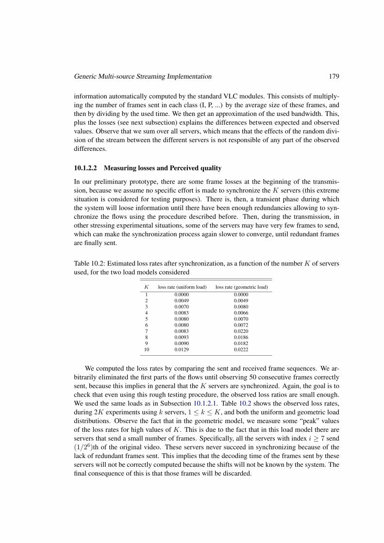
Generic Multi-source Streaming Implementation 179
information automatically computed by the standard VLC modules. This consists of multiply-ing the number of frames sent in each class (I, P, ...) by the average size of these frames, andthen by dividing by the used time. We then get an approximation of the used bandwidth. This,plus the losses (see next subsection) explains the differences between expected and observedvalues. Observe that we sum over all servers, which means that the effects of the random divi-sion of the stream between the different servers is not responsible of any part of the observeddifferences.
10.1.2.2 Measuring losses and Perceived quality
In our preliminary prototype, there are some frame losses at the beginning of the transmis-sion, because we assume no specific effort is made to synchronize the K servers (this extremesituation is considered for testing purposes). There is, then, a transient phase during whichthe system will loose information until there have been enough redundancies allowing to syn-chronize the flows using the procedure described before. Then, during the transmission, inother stressing experimental situations, some of the servers may have very few frames to send,which can make the synchronization process again slower to converge, until redundant framesare finally sent.
Table 10.2: Estimated loss rates after synchronization, as a function of the numberK of serversused, for the two load models considered
K loss rate (uniform load) loss rate (geometric load)1 0.0000 0.00002 0.0049 0.00493 0.0070 0.00804 0.0083 0.00665 0.0080 0.00706 0.0080 0.00727 0.0083 0.02208 0.0093 0.01869 0.0090 0.0182
10 0.0129 0.0222
We computed the loss rates by comparing the sent and received frame sequences. We ar-bitrarily eliminated the first parts of the flows until observing 50 consecutive frames correctlysent, because this implies in general that the K servers are synchronized. Again, the goal is tocheck that even using this rough testing procedure, the observed loss ratios are small enough.We used the same loads as in Subsection 10.1.2.1. Table 10.2 shows the observed loss rates,during 2K experiments using k servers, 1 ≤ k ≤ K, and both the uniform and geometric loaddistributions. Observe the fact that in the geometric model, we measure some “peak” valuesof the loss rates for high values of K. This is due to the fact that in this load model there areservers that send a small number of frames. Specifically, all the servers with index i ≥ 7 send(1/26)th of the original video. These servers never succeed in synchronizing because of thelack of redundant frames sent. This implies that the decoding time of the frames sent by theseservers will not be correctly computed because the shifts will not be known by the system. Thefinal consequence of this is that those frames will be discarded.

180 GOL!P2P: A P2P Prototype for Robust Delivery High Quality Live Video
We consider the perceived quality of the reconstructed stream. In Section 5.2.3, we ap-ply the PSQA technology, obtaining a simple function, Q(LR,MLBS ), that maps the lossrate, LR, and the mean lost burst size, MLBS , into the perceived quality. Consider the lossrates obtained using the uniform load model, as shown in Table 10.2. The worst case is whenMLBS = 1 (see Figure 5.6 that plot the PSQA simple function). Using this MLBS value andthe loss rates given in the first column of Table 10.2, we obtain, as perceived quality estimates,values going from 10 (maximal quality) to approximately 9, which is almost maximal. For thegeometric load (somehow an extreme situation), we observe loss ratios up to 0.0222, which inthe worst case of MLBS = 1, translates into a quality level of about 5 (this corresponds to thecharacterization “fair” in the subjective testing area). The reason was already commented: theservers having little to send have no time to synchronize. This is telling us that the losses due tothe synchronization problem we observed, even if the situation which generated them is a littlebit too pessimistic, should be diminished. This is commented in the last concluding section.
These measures show that the present implementation needs some improvements to reducethe losses due to the possible lack of synchronization (even if they are not very important innumber). In order to diminish these losses, we are currently working on adding extra redun-dancy for a better synchronization (for instance, by sending at the beginning, all the framesby all the servers, during some pre-specified time or until a pre-chosen number of frames havebeen sent). Also, when a server has almost no frame to send, we also can force it to sendredundant data, again for allowing the client to estimate the drifts with sufficient accuracy.
10.2 GOL!P2P Architecture: a Tree-based Structured Overlay Peer-to-Peer System
This section presents our full video delivery network based on a Peer-to-Peer architecture,called GOL!P2P. It is the integration effort of the methodologies developed in the previouschapters. Our prototype is a completely free-software application, based on well-known tech-nologies which can be executed on various operating systems.
GOL!P2P is a new approach of P2PTV networks, based on the quality perceived by finalusers. We measure, in real time and automatically, the perceived quality at the client side bymeans of the PSQA technology. Moreover, we improve the efficiency and robustness of thenetwork, in terms of the quality it delivers, considering the lifetime clients behavior of a realsystem.
Our design mitigates the impact of the peer’ disconnection at two levels. In the long termthe system places the peers most compromised with the network (those with largest lifetimeand smallest bandwidth fluctuation) near to the broadcaster, in order to obtain a more robustoverlay topology. This dynamics is formalized as a mathematical optimization problem whichis solved in Chapter 8. In the short term, and once defined which peers will serve the streamingto each client, we study the best streaming technique that mitigates the peers’ disconnections.Our delivery scheme was called multi-source streaming technique; an optimal configuration of
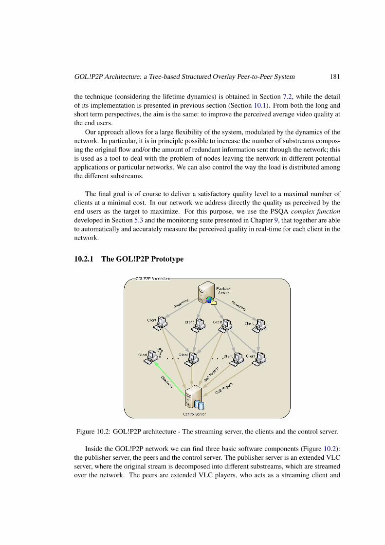
GOL!P2P Architecture: a Tree-based Structured Overlay Peer-to-Peer System 181
the technique (considering the lifetime dynamics) is obtained in Section 7.2, while the detailof its implementation is presented in previous section (Section 10.1). From both the long andshort term perspectives, the aim is the same: to improve the perceived average video quality atthe end users.
Our approach allows for a large flexibility of the system, modulated by the dynamics of thenetwork. In particular, it is in principle possible to increase the number of substreams compos-ing the original flow and/or the amount of redundant information sent through the network; thisis used as a tool to deal with the problem of nodes leaving the network in different potentialapplications or particular networks. We can also control the way the load is distributed amongthe different substreams.
The final goal is of course to deliver a satisfactory quality level to a maximal number ofclients at a minimal cost. In our network we address directly the quality as perceived by theend users as the target to maximize. For this purpose, we use the PSQA complex functiondeveloped in Section 5.3 and the monitoring suite presented in Chapter 9, that together are ableto automatically and accurately measure the perceived quality in real-time for each client in thenetwork.
10.2.1 The GOL!P2P Prototype
Figure 10.2: GOL!P2P architecture - The streaming server, the clients and the control server.
Inside the GOL!P2P network we can find three basic software components (Figure 10.2):the publisher server, the peers and the control server. The publisher server is an extended VLCserver, where the original stream is decomposed into different substreams, which are streamedover the network. The peers are extended VLC players, who acts as a streaming client and

182 GOL!P2P: A P2P Prototype for Robust Delivery High Quality Live Video
server at the same time. Initially the peers take directives from the control server in order toknow where to receive the substreams from. During the execution, each peer receives multiplesubstreams and using the multiple source approach it builds the original stream before playingit. Also the peers can send each of the substreams to other clients. The control server is thecentral manager of the P2P network, responsible in particular of its topology. The perceivedquality in the network is audited automatically and in real-time at the control server, usingperiodical information sent by peers.
Publisher Server. As shown in Figure 10.3, we separate the publisher server into two dif-ferent components, the broadcaster and the splitter. The broadcaster takes the content froma source and inserts user-data into the stream, which is used by the clients to measure thelosses per frame type. All content sources are supported, such as a stored content or a livecontent or an Internet streaming. In our case we use a stored MPEG-4 content. The splitterdecomposes the stream in sub-streams according to the previously described algorithm (Sub-section 10.1.1.1). It also acts as the root node (also called node 0) inside the tree-based overlay.Both components are plugged VLC modules.
Figure 10.3: Publisher server architecture.
Peers Peers (clients) interact with the control server, implement the measurement procedures(for building the PSQA metric) and reconstruct the stream for playing it. As shown in Fig-ure 10.4, three main modules were added to the VLC player for this purpose: the control mod-ule, the multisource module and the measurement module. The control module is in chargeof the communication between the control server and the peers. It periodically reports (to thecontrol server) the QoS parameters measured within a peer and also read directives from thecontrol server (for instance, routing information). All communications between the peers andthe control server are done over HTTP. The multisource module is capable of reconstructingthe original stream (with the procedure described in Subsection 10.1.1.2) from the set of sub-streams, or a degraded version of it if some of the substreams had losses, or are simply missing.The measurement module is where all streams measurements are done. Inside this module theuser-data inserted in the broadcaster server are parsed and used in order to calculate the lossrates. Finally in order to stream the substreams received to other clients, a VLC module calledstandard stream output is used.
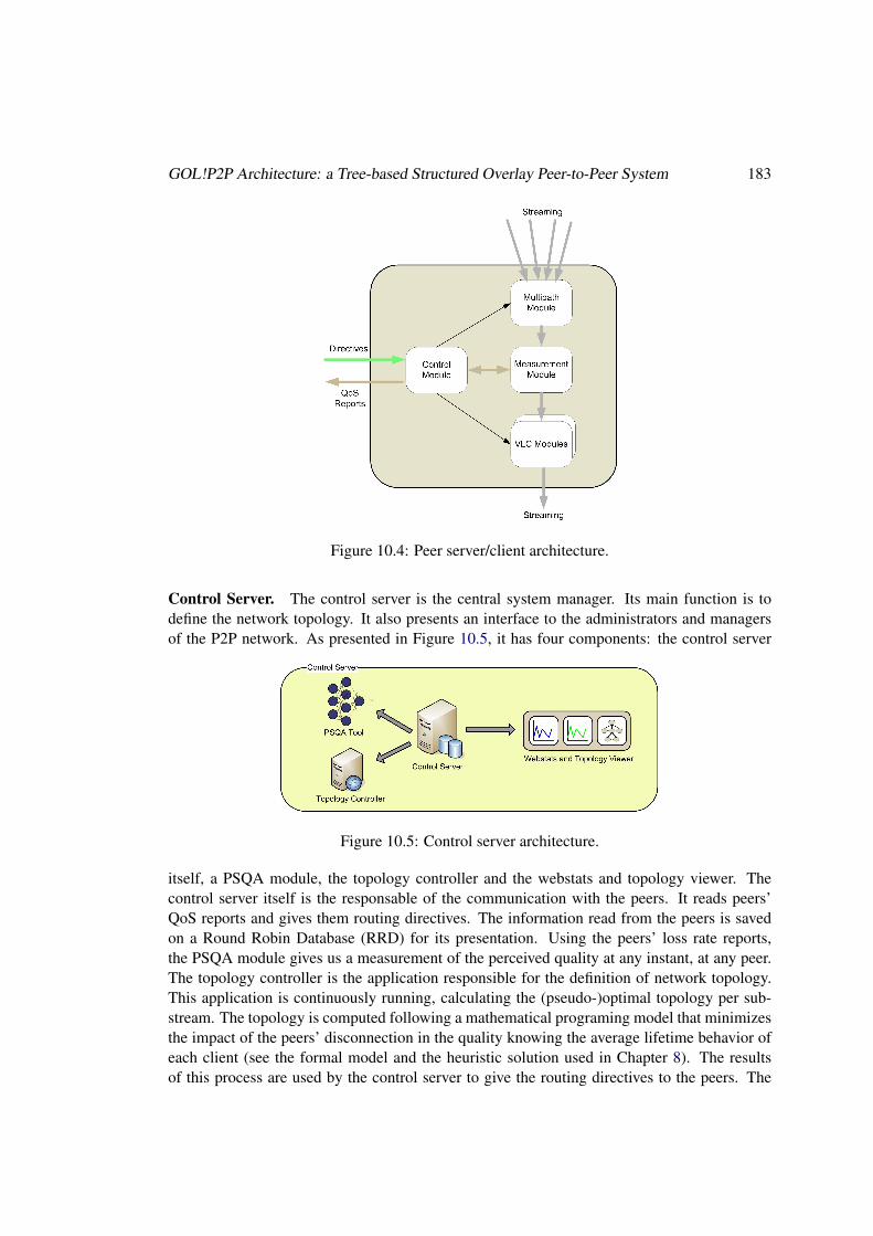
GOL!P2P Architecture: a Tree-based Structured Overlay Peer-to-Peer System 183
Figure 10.4: Peer server/client architecture.
Control Server. The control server is the central system manager. Its main function is todefine the network topology. It also presents an interface to the administrators and managersof the P2P network. As presented in Figure 10.5, it has four components: the control server
Figure 10.5: Control server architecture.
itself, a PSQA module, the topology controller and the webstats and topology viewer. Thecontrol server itself is the responsable of the communication with the peers. It reads peers’QoS reports and gives them routing directives. The information read from the peers is savedon a Round Robin Database (RRD) for its presentation. Using the peers’ loss rate reports,the PSQA module gives us a measurement of the perceived quality at any instant, at any peer.The topology controller is the application responsible for the definition of network topology.This application is continuously running, calculating the (pseudo-)optimal topology per sub-stream. The topology is computed following a mathematical programing model that minimizesthe impact of the peers’ disconnection in the quality knowing the average lifetime behavior ofeach client (see the formal model and the heuristic solution used in Chapter 8). The resultsof this process are used by the control server to give the routing directives to the peers. The

184 GOL!P2P: A P2P Prototype for Robust Delivery High Quality Live Video
webstat and topology viewer is an application designed to present the data gathered by thecontrol server and the network topology defined by the topology calculator to administratorsand managers of the GOL!P2P network. It offers reports at different levels and types of views.It is possible to generate reports focused on a particular stream or on a specific client (wherethere could be more than one active stream), or perhaps on the entire network (where therecould be more than one client). Finally it is possible to display the results at the frame level,possibly per frame type (I, P, B), or at the PSQA level.
Implementation. As mentioned before, clients and servers are based on VLC code. Thelibavcodec (ffmpeg) library was used in order to work with MPEG-2/4 video specifica-tions. The container format was MPEG-TS, using the functionalities provided by libdvbps.We streamed over HTTP and UDP using VLC internal modules. The control server and web-stat are written in PHP; they use MySQL and Oracle Berkeley Databases and both of them runover Apache. We used the RRDtool to generate the statistical graphs and Graphviz to visualizethe network topology. As a difference with the monitoring suite presented in Chapter 9, the pe-riodical reports sent by peers to the control server are delivered over HTTP as a piggybackinginformation of the directives, instead of SNMP3. The GOL!P2P application can be easily ex-tended to support other container formats (MPEG-PS, OGM...) and transport protocols (RTP,MMS...). All libraries and applications mentioned above are free-software and they can beexecuted in Microsoft Windows, Unix, Linux, etc.
10.3 Extending Frontiers: Improving our Video Delivery Refer-ence Service
In this section we test our GOL!P2P prototype. Using our P2P client and servers implemen-tation, we deliver video on the Internet, and we verify the correct integration of each piece ofsoftware. The tests are divided into client-level and network-level tests. The former exploreproperties of the prototype from the user point of view, such as reconnection time, theoreticalversus observed quality values, bandwidth consumption, etc. The latter refer to the global per-formance of the network, for instance the average behavior of the peers, the scalability of thenetwork when the quantity of peers grows, etc.
All the tests were done in PlanetLab [259]. PlanetLab is a global research network thatsupports the development and test of new network services. It currently consists of 813 nodesat 401 sites. The peers’ dynamics is based on the live-video service presented in Section 2.5.
To distribute the video, we use six different multi-source streaming configurations. We usethe optimal configurations specified in Table 7.11, forK ∈ {1, 2, 3, 4, 5, 8} (see Section 7.2 fordetails about the procedure followed to obtain these configurations). We decide not to applyredundancy in these tests r = 0% because of strong limitations in the available bandwidth ineach node of Planetlab. The bitrate of the original stream (and therefore, the overall bandwidth
3In this case we audit all the clients, not just a set of probes, an SNMP approach will not perform well.

Extending Frontiers: Improving our Video Delivery Reference Service 185
considering all the sub-streams) is 512 kbps. There is no constraint on the upload bandwidth ofthe multi-source streaming configurations chosen. Table 10.3 shows the bandwidth consumedper sub-stream for each configuration.
Table 10.3: Upload bandwidth consumed on server i, for the multi-source streaming techniquedefined in Table 7.11, with K sub-streams and r = 0%.
i/K 1 2 3 4 5
1 492.7 170.6 73.1 34.1 16.52 341.3 146.3 68.1 33.03 292.6 136.2 66.04 272.4 132.05 263.7
total 492.7 511.9 512.0 510.8 511.3
i/K 6 7 8 9 10
1 8.1 4.0 2.0 1.0 0.52 16.2 8.1 4.0 2.0 1.03 32.5 16.1 8.0 4.0 2.04 65.0 32.2 16.0 8.0 4.05 129.9 64.4 32.1 16.0 8.06 259.9 128.9 64.2 32.1 15.97 257.8 128.4 64.1 31.98 256.7 128.2 63.79 256.5 127.410 254.9
total 511.7 511.5 511.4 512.0 509.3
As in Section 8.4, we can compute a “theoretical” value of the perceived quality depending onwhich sub-stream is received by the user. For instance, if K = 1, an user has perfect qualitywhen he/she receives the stream, and zero quality otherwise. We compute these “theoreti-cal” values from the PSQA complex function, of Section 5.3.3, using the loss process modeldescribed in Section 7.2. Next subsections compare these values with the measured ones.
10.3.1 Client Performance Tests
We performed two families of tests concerning the clients’ point of view: the first one concernsthe impact of the peers’ disconnections; the second one looks at the impact of the distance(the delay) in the network between the peer servers and the client. Each test instance has aduration of 4 minutes, and it uses the multi-source streaming technique specified in the fourthrow (K = 4) of Table 7.11.
The peers’ disconnection dynamics. In this test, we have four peers sending a different sub-stream each to a client. To measure the impact of peer disconnections in the perceived quality,we disconnect each of the sources separately and measure, in the client, the perceived qualityand the reconnection time. Figure 10.6 shows the measured PSQA when one of the serversdisconnects from the network. Quality degrades to 0.5 (PSQA scaled in [0, 1]), but this is fora short period because the network will quickly replace the disconnected peer with anotherconnected peer.
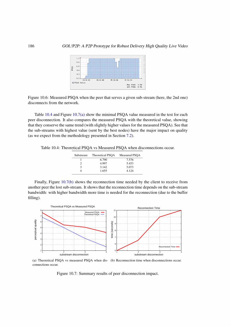
186 GOL!P2P: A P2P Prototype for Robust Delivery High Quality Live Video
Figure 10.6: Measured PSQA when the peer that serves a given sub-stream (here, the 2nd one)disconnects from the network.
Table 10.4 and Figure 10.7(a) show the minimal PSQA value measured in the test for eachpeer disconnection. It also compares the measured PSQA with the theoretical value, showingthat they conserve the same trend (with slightly higher values for the measured PSQA). See thatthe sub-streams with highest value (sent by the best nodes) have the major impact on quality(as we expect from the methodology presented in Section 7.2).
Table 10.4: Theoretical PSQA vs Measured PSQA when disconnections occur.
Substream Theoretical PSQA Measured PSQA1 6.790 7.5762 4.997 5.4533 3.142 5.0734 1.655 4.124
Finally, Figure 10.7(b) shows the reconnection time needed by the client to receive fromanother peer the lost sub-stream. It shows that the reconnection time depends on the sub-streambandwidth: with higher bandwidth more time is needed for the reconnection (due to the bufferfilling).
1
2
3
4
5
6
7
8
1 2 3 4
perc
eptu
al q
ualit
y
substream disconnection
Theoretical PSQA vs Measured PSQA
Measured PSQATheoretical PSQA
(a) Theoretical PSQA vs measured PSQA when dis-connections occur.
5
6
7
8
9
10
11
1 2 3 4
time
(sec
onds
)
substream disconnection
Reconnection Time
Reconnection Time
(b) Reconnection time when disconnections occur.
Figure 10.7: Summary results of peer disconnection impact.

Extending Frontiers: Improving our Video Delivery Reference Service 187
The peers’ inter-delay. In this test, we have the same overlay topology and configurationas before. But we place the peers in two different geographical location scenarios, one closeto the client, the other one far from it. The distances between the nodes are measured as thecorresponding end-to-end delays, calculated by averaging the round trip time of ICMP packets.To measure the impact of the delay in the perceived quality, we disconnect each of the fourservers separately and measure, at the client’s side, the perceived quality and the reconnectiontime. The delay from the peers to the client of the two scenarios, called “close” and “far”, aresummarized in Table 10.5.
Table 10.5: Delay from the peers to the client in our two scenarios.
Peer Distance (ms)“close” “far”
peer 1 21.0 266peer 2 28.1 281peer 3 28.1 281peer 4 27.9 281
peer of reconnection 0 0.15 273
The mean/median/minimal perceived quality at the client side is measured with the PSQAtechnique. The connection and reconnection times of the multi-source streaming technique arealso measured. The results of the tests show no significant impact of the delay in the perceivedquality. The tests show no impact in the reconnection time neither. For instance, in Table 10.6we show the results when peer “1” is disconnected. We show the average measurements in
Table 10.6: Peers’ inter-delay measurements.
Periodsmeasure without with total
disc. disc.
“close” scenariomean PSQA 9.947 6.543 8.812median PSQA 10.000 6.454 10.000min PSQA 9.209 4.678 4.678theoretical PSQA 10.000 6.790 -connection time (sec.) - - 8.5reconnection time (sec.) - 16 -
“far” scenariomean PSQA 9.988 6.500 8.825median PSQA 10.000 5.566 10.000min PSQA 9.632 5.068 5.068theoretical PSQA 10.000 6.790 -connection time (sec.) - - 9reconnection time (sec.) - 12 -
the period without disconnections and in the period with disconnections. In the two scenarios,“close” and “far”, the quality measurements have negligible differences, and, as we expected,the connection time (streaming start-up) is shorter in the “close” scenario. But, surprisingly,the reconnection time is longer in the “close” scenario than in the “far” scenario. This behavior

188 GOL!P2P: A P2P Prototype for Robust Delivery High Quality Live Video
is justified because the delay time is negligible with respect to other factors, as for instancewith respect to the central network reconfiguration time, or to the buffering time.
10.3.2 Network Behavior Tests
We performed two tests that evaluated the performance and scalability of the global network.The first test evaluates the performance of the network when different configurations of themulti-source streaming technique are used. The second test determines the impact of the peers’connection dynamics in the global quality of the network. Each test instance has a duration of400 seconds.
The number of sub-streams. In this test, we have 30 peers with a specific connection/disconnectiondynamics extracted from a real situation. In Figure 10.8 we show the number of clients con-nected to the network, varying between 17 and 21 simultaneous connections. Each peer exe-cutes in a particular Planetlab node.
Figure 10.8: Number of clients connected to the network.
Using the same peers dynamics, we tried six different multi-source streaming configura-tions and evaluated the performance of each case. The configurations used correspond to thenumber of sub-streams in K ∈ {1, 2, 3, 4, 5, 8}, Table 7.11.
We evaluated the mean and the median PSQA of all the connected peers in the streamingperiod (the streaming has a duration of 400 seconds). Figure 10.9 shows the results. Theschemes with two, three and four sub-streams show the best performance.
Figures 10.10(a) and 10.10(b) explain why the quality does not increase with the number ofsub-streams. Figure 10.10(a) shows the number of clients that don’t receive all the sub-streamsbecause of the disconnection of another peer. Considering only 30 nodes in the network, witha fixed connection/disconnection dynamics, when the number of sub-streams increases theprobability of been served from a peer that will be disconnected also increases. Therefore,when the number of sub-streams increases, more clients will probably have losses because ofother peers’ disconnections. But this doesn’t imply a global degradation of the quality.
The topology of the network is computed (by the control server) by means of the greedyalgorithm explained in Chapter 8. When the number of sub-streams increases, the number ofpossible topologies also increases. This means that, potentially, more intelligent assignmentscan be done, but also more computation time is needed at the control server for the topologycalculation. Figure 10.10(b) shows the time needed by the control server to connect a client

Extending Frontiers: Improving our Video Delivery Reference Service 189
8.0
8.2
8.4
8.6
8.8
9.0
9.2
9.4
9.6
9.8
10
1 2 3 4 5 6 7 8
perc
eptu
al q
ualit
y
number of substreams
Measured PSQA for different number of substreams
Mean PSQAMedian PSQA
Figure 10.9: PSQA measured for each schema tested.
0
2
4
6
8
10
12
14
16
18
20
1 2 3 4 5 6 7 8
clie
nts
with
a le
ast o
ne
serv
er d
isco
nnec
tion
number of substreams
Number of Clients with a least one server disconnection
(a) [Number of clients with at least one disconnectionpeer.
0
5
10
15
20
25
30
1 2 3 4 5 6 7 8
time
(sec
onds
)
number of substreams
Connection Time measured for different number of substreams
Mean Connection TimeMean Reconnection Time
(b) Connection time.
Figure 10.10: Connection time and number of clients with at least one disconnection peer pernumber of sub-streams.

190 GOL!P2P: A P2P Prototype for Robust Delivery High Quality Live Video
(at the first time or after a peer’ disconnection). This time basically consists in the topologycomputation time. When the original streaming is used (there is only one sub-stream), there areonly five clients who loose the peer that serve their streaming, and therefore they do not receiveanything (the other clients receive the streaming perfectly). The connection and reconnectiontime is also very low for this scheme (between 10 and 5 seconds). But the average globalperformance of the one sub-stream scheme is very poor because these five clients have theworst quality (zero) in the failure period. In the four sub-streams scheme only the leaves inthe graph disconnect (and therefore there are no losses and reconnection time). But, when thenumber of sub-streams increases, the computation time (the connection and reconnection time)increases, and therefore the losses impact in a longer period. For the schemes with five sub-streams and more, there are too many disturbed clients because of other peers’ disconnections,and despite of the fact that these disconnections only affect in part the streaming quality, theaverage global quality decreases.
The peers’ connection/disconnection dynamics. In this test, we use again the multi-sourcestreaming technique with the configuration given in the fourth row of the Table 7.11, whichhas four sub-streams. To measure the impact of the peers’ connection/disconnection dynamicsin the perceived quality, we evaluate four real scenarios with different dynamics. Table 10.7shows the number of peers’ connections and peers’ disconnection for each scenario.
Table 10.7: Peers’ connection/disconnection dynamics in the four network tests scenarios.
scenario total client total clientconnections disconnections
1 30 62 41 103 49 144 70 59
Each test instance has a duration of 400 seconds. For each test, we measure the averagemean and median perceived quality for all the peers. Table 10.8 and Figure 10.11 present theresults. As we expected, the average perceived quality decreases when the network’ dynamicsincreases.
Table 10.8: Measured PSQA for each scenario.
Scenario Mean PSQA Median PSQA1 8.7 9.32 8.0 8.83 7.9 8.14 6.8 7.1
Extending our Reference Service Network with our Hybrid GOL!P2P Prototype. Thenetwork behavior tests demonstrate the capability of our prototype to extend a Content DeliveryNetwork infrastructure in real scenarios. The fresh clients bandwidth can be used to deliver
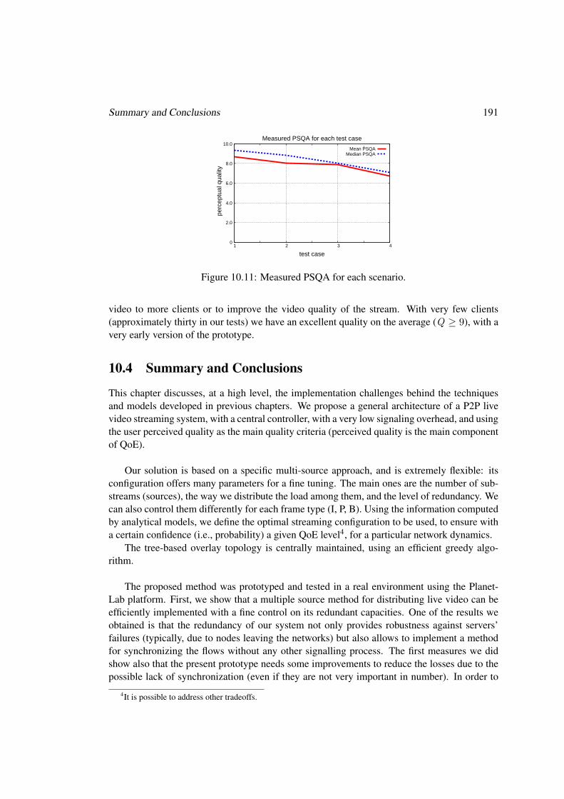
Summary and Conclusions 191
0
2.0
4.0
6.0
8.0
10.0
1 2 3 4
perc
eptu
al q
ualit
y
test case
Measured PSQA for each test case
Mean PSQAMedian PSQA
Figure 10.11: Measured PSQA for each scenario.
video to more clients or to improve the video quality of the stream. With very few clients(approximately thirty in our tests) we have an excellent quality on the average (Q ≥ 9), with avery early version of the prototype.
10.4 Summary and Conclusions
This chapter discusses, at a high level, the implementation challenges behind the techniquesand models developed in previous chapters. We propose a general architecture of a P2P livevideo streaming system, with a central controller, with a very low signaling overhead, and usingthe user perceived quality as the main quality criteria (perceived quality is the main componentof QoE).
Our solution is based on a specific multi-source approach, and is extremely flexible: itsconfiguration offers many parameters for a fine tuning. The main ones are the number of sub-streams (sources), the way we distribute the load among them, and the level of redundancy. Wecan also control them differently for each frame type (I, P, B). Using the information computedby analytical models, we define the optimal streaming configuration to be used, to ensure witha certain confidence (i.e., probability) a given QoE level4, for a particular network dynamics.
The tree-based overlay topology is centrally maintained, using an efficient greedy algo-rithm.
The proposed method was prototyped and tested in a real environment using the Planet-Lab platform. First, we show that a multiple source method for distributing live video can beefficiently implemented with a fine control on its redundant capacities. One of the results weobtained is that the redundancy of our system not only provides robustness against servers’failures (typically, due to nodes leaving the networks) but also allows to implement a methodfor synchronizing the flows without any other signalling process. The first measures we didshow also that the present prototype needs some improvements to reduce the losses due to thepossible lack of synchronization (even if they are not very important in number). In order to
4It is possible to address other tradeoffs.

192 GOL!P2P: A P2P Prototype for Robust Delivery High Quality Live Video
diminish these losses, we are currently working on adding extra redundancy for a better syn-chronization (for instance, by sending at the beginning, all the frames by all the servers, duringsome pre-specified time or until a pre-chosen number of frames have been sent). Also, whena server has almost no frame to send, we can force it to send redundant data, again allowingthe client to estimate the drifts with enough accuracy for avoid losses due to synchronization.Second, with respect to the global system, some preliminary results show the feasibility of theprototype capability for real life usage. Client level and network level tests validate the modelsand methodologies used. All the results show a very good behavior from the perceptual qualitypoint of view, allowing us to think that extending a CDN with a P2P distribution will be acommon feature in the near future.

Chapter 11
Challenges in VoD and MyTV services
In the previous chapters we studied different aspects of a broadcast video service. Live videostreaming is one of the most challenging services, because of its bandwidth consumption andof its real-time restrictions. But present day Video Delivery Networks must provide a series ofcomplementary services.
In this chapter, we study Video on Demand (VoD) and MyTV complementary services.In particular, we focus on a caching search strategy for these services, because the contentdiscovery is the largest challenge here. In Section 11.2 we present a model of the impact thatcache expiration times have on the total number of correct answers to queries in a contentnetwork, and on the bandwidth usage. We develop a mathematical programming formulationof the model, which is tested in Section 11.4 with a set of P2P test cases and a DNS systemcase coming from real traces.
The state of the art of content discovery and some models have been presented at three con-ferences: 33th Argentine Conference on Computer Science and Operational Research (JAIIO’04),Jornadas de Informática e Investigación Operativa (JIIO’04), and XIII Congreso Latino-Ibero-americano de Investigación Operativa (CLAIO’06) [276, 277, 279] (listed at the Introduction as[jaiio04] [jiio04][claio06]). The mathematical programming model of cache expiration timeshas been published at the International Network Optimization Conference (INOC’07) [280](listed at the Introduction as [inoc07]). The file-sharing P2P system test scenario has been pre-sented at the 3rd international IFIP/ACM Latin American conference on Networking (LANC’05)[278] (listed at the Introduction as [lanc05]). The Domain Name System (DNS) test scenariohas been presented at the 3rd international conference on the Quantitative Evaluation of Sys-tems (QEST’06) [42] (listed at the Introduction as [qest06]).
11.1 Video-on-Demand and MyTV services
Interactive TV has different meanings depending on the VDN capabilities and user behaviors.Some services are essentials for the next generation of VDN’s, the most important are:
Electronic Program Guide (EPG). The Electronic Program Guide (EPG) is an on-screenguide to scheduled broadcast programs, allowing a viewer to navigate, select, and searchcontent by time, title, channel, genre, etc.
193

194 Challenges in VoD and MyTV services
In our P2P context, this service is very simple to implement: It can be implemented usinga traditional Web Server-Client approach of some variants of Podcasting or Broadcatch-ing (see section 11.1.1).
Time Shift TV (TSTV). Time shifting is the capability of recording, pausing, playing andrewinding a live broadcast streaming for short periods, giving the possibility to be viewedtwice or at a time more convenient to the user.
Personal Video Recorder (PVR). Personal Video recorder, also know as Digital Video Recorder(DVR), it is the capability of recording a broadcast streaming for a long period to beplayed after by the user. As TSTV, PVR provides basic media player functionalities(pause, fast forward, fast rewind, slow forward, slow rewind, etc.). In some VDN’s, in-stead of having the recording capability in the customer device (knows as a Set-top-box),these functionalities are implemented in the network. This special kind of PVR is knowsas Network Personal Video Recorder (NPVR), and its development has been motivatedby economical reasons.
To add TSTV and PVR functionalities to our prototype is an easy task. Because, in ourP2P network, the user device is a computer, and it is possible to record a streaming withany multimedia player, particullary with the VideoLan Client. In this case, there is noneed to implement NPVR.
Video on Demand (VoD). Video on Demand allow users to watch pre-stored movies or tele-vision programs that are available in the VDN. First, the user discovers the video thathe wants to watch, selects it, and finally a unicast streaming or progressive download(depending on the kind of network) starts from the network to user. VoD services pro-vide the user with traditional PVR functionality (pause, fast forward, fast rewind, slowforward, slow rewind, jump to previous/future chaper, etc.). In some VDN’s is not pos-sible to implement a unicast stream or progressive download, a variant of VoD calledNear Video on Demand (NVoD) is used in these networks. NVoD is implemented witha multicast streaming, when a user selects a video to watch, he has to wait until the nextmulticast streaming of this video starts, implying that NVoD is only suitable for verypopular videos. Push video on demand (PVoD) is used, in systems that lack interactivity,to emulate the VoD service. PVoD uses a Personal Video Recorder (PVR), at the userhome, to record pre-defined videos (often transmitted at the night idle capacity). Theuser can then watch the downloaded videos at a time of their choosing.
VoD is a high bandwith resource consuming service. In spite of being very attractive forthe users, its implementation is limited to some new VDN’s. Essentially, VoD is a specialcase of file distribution, with very light real-time constraints. This allows that the VoDshould be implemented in almost all Content Delivery Network (CDN) and Peer-to-Peerfile sharing systems. In our context a P2P solution is the most suitable. Internet-basedVoD services allow to the user of offering his own videos. The main technical problemis that peers connect and disconnect with high frequencies, and then, the videos that theypublish are also highly variable. And thus, that to discover and to download a video of thenetwork can be a difficult task. This is the main challenge in P2P design for VoD: to offer

Video-on-Demand and MyTV services 195
the content needed by the clients in a highly varying environment. Efficient download ina file-sharing P2P network was widely studied (see for instance [15, 47, 209, 216]). Inthis chapter we study the impact of the content dynamics in the search performance, i.e.the content discovery1.
Pay per View (PPV). Pay per view is the service in which users can purchase broadcast eventsto be seen on TV and pay for the private view of that event to their homes. The event isshown at the same time to everyone ordering it, as opposed to video on demand service,which allows viewers to see the event at any time.
PPV adds the technological need for a Billing System and a Digital Right Management(i.e. a encrypted streaming method and the management of the associate encryption key).PPV implementation over a P2P network is possible, for instance Joost [185] and newBitTorrent [31] have this technology.
MyTV. MyTV (also know as ShareTV or selfcast) is the possibility to the user of offering itown broadcast channel. As an extension of the video-conference, MyTV is suitable forfamiliar events, or for small producers.
The Streaming of MyTV service can be high bandwidth consuming. From a technicalpoint of view, it can be implemented like any broadcast streaming, therefore in our sharedresource P2P approach it is not a problem. But MyTV service has the same problem thanthe VoD service, with high dynamics in the contents. In this chapter we also study thesearch performance for MyTV service.
Others. A lot of interactive services are developed today for the next generation VDN’s. Forexample multi-player games, voting, interactive advertising, etc.
In the rest of the chapter we study the content discovery for the VoD and MyTV services.
11.1.1 Making Content Accessible: Video Podcast and Broadcatching are notenough
Video podcast2 , also called vodcast, is a online announcing mechanism for video on demand(VoD), where the clients automatically discover new files. The client subscribes to a channel,where he receives regular programs. The client can view these programs at his own leisure.It can be considered as an Internet equivalent of a broadcast medium, and specifically of theTime Shift TV service3.
In podcasting, the content publisher begins by making a video file available to delivery onthe network through some known Uniform Resource Identifier (URI). Then, the content pub-lisher announces the existence of that video file by referencing it in a web feed. The web feedis a XML file that provides a list of URIs with additional information (such as title, description,
1Specially in the case when the clients can submit their own videos.2The word “PodCasting” is a merger of the words PoD (Portable on Demand) and broadcasting. The iPod, of
Apple Inc., owes its name to the PoD concept. The first podcasting service was developed for the iPod. Today,podcast is no longer specifically related to the iPod.
3Some Personal Video Recorders (PVRs), such as TiVo, allow podcasting as a new service.
196 Challenges in VoD and MyTV services
and publish date). The web feed is generally published via Really Simple Syndication (RSS),or via the proposed standard [160, 163] Atom Syndication Format (Atom).
Syndication of the video on demand has benefits for both publishers and clients. Pub-lishers can automatically announce content for their subscribers. Moreover, they can providededicated content depending on each specific client interest. Clients can easily discover selec-tive content, and merge content from different publishers (broadcatching allows a many-to-onecommunication instead the traditional one-to-many of the broadcasting).
Extending the video podcasting concept, broadcatching is the automated download ofcontent that has been made available on the network using podcasting.
Broadcatching allows a complete and easy to use solution, for the discovery and distri-bution of the video on demand. The technology is easy adaptable to a P2P network. A firstintegration can be a centralized server syndication (using the standard RSS mechanism) whereeach URI listed in the web feed is actually an identifier of the file in a P2P distribution network(for instance a .torrent file in a Bittorrent network). A better integration can be the elimina-tion of the inefficient polling of the RSS feed in the central server, and the distribution of thefeed also with the P2P network. A light notification can be sent to each client (typically viaXML-RPC) to announce the new web feed. Then the client downloads the web feed from theP2P network, and after, the client automatically downloads the content, from the P2P network,following the instructions in the feed.
But, as we see, broadcatching does not adapt well to very dynamic content. Today, asuccessful video delivery network has to allow users to publish their own content (not only thecontent of the content provider), already be in the form of video on demand (VoD) or live TVchannels (MyTV). VoD of user content has the same design challenges that actual file-sharingP2P systems, where the content and the peers has high dynamics. A efficient distribution canbe achieved using peer-to-peer technologies, but the discovery of the dynamic content cannot be implemented with traditional announcement methods (like podcasting). Instead, searchmechanisms have to be implemented in the network, in order to obtain an efficient discovery ofthe dynamic content. The same situation happen with the MyTV service, with the differencethat the distribution on the P2P network is similar to the live TV distribution (instead of thefile-sharing distribution).
11.1.2 Using a Search Caching approach: Network Structure Roles and Work-load
As we have previously discussed (in Section 2.3), in a Content Network the addressing androuting are based on the content description, instead of on its location. This means that everycontent network is actually a knowledge network, where the knowledge is the informationabout the location of the nodes where each specific content is to be found: this is "meta-information", in the sense of being the information about the information contents themselves.The objective of the network is to be able to answer each content query with the most completepossible set of nodes where this content is to be found. This corresponds to discover thecontent location in the most effective and efficient possible way. There are two main strategies

Making Video Libraries Efficiently Searchable 197
to discover the meta-information, namely publication and search. By publication we meanthe process by which a network node unrequestedly sends meta-information it possesses to theremaining nodes (for instance, broadcatching). By search we mean the process by which a nodeasks the remaining ones to send it the meta-information they possess. By analogy with logistics,we can say that publication is an “information push” strategy, and search an “information pull”strategy. As both nodes and contents are continuously going in and out of the network, thetask of maintaining updated the network meta-information is very difficult and represents animportant communication cost. Both publishing and search can contribute towards this task, buttheir relative efficiency varies, so that there is a tradeoff between their frequency and modalityof application. In this context, cache nodes are used to hold the available meta-information. Asthis information is continuously getting outdated, the cache nodes must decide when to discardit, which means increasing communication overhead for the sake of improving the quality ofthe answers.
In this chapter, we develop a simplified model of a content network, and in particular ofthe number of correct answers to a query as a function of the information expiration times usedat the cache nodes, presented in Section 11.2. To the best of our knowledge, this is an aspectthat has not been previously treated analytically in the literature (see our study of the relatedwork on Section 11.3). This model gives rise to a mathematical programming formulation,which can be used to find the expiration times maximizing the correct answers to the queriesreceived. Two numerical illustration are shown in Section 11.4. One is based on a file-sharingP2P system, that presents a similar dynamics to the expected dynamics in the VoD service (withcontent uploaded by the users). The other one is based on the DNS system, with a dynamicsbehavior similar to the MyTV service. The chapter concludes, in Section 11.5, with generalresults and discussion.
11.2 Making Video Libraries Efficiently Searchable
This section formalizes the problem of caching meta-information in a content network in orderto maximize the number of correct answers to the queries, while respecting the bandwidthconstraints; this will be our Content Caching Problem (CCP ).
11.2.1 Preliminary Definitions
Network components description. We will look at the content network as composed ofsource nodes and querying nodes (which may be the same), of cache nodes (also called aggre-gation nodes), and of a backbone (which will not be further modeled); a graphical representa-tion can be seen in Figure 11.1. This division is actually virtual, as a same physical node mayact at the same time as a source node, a querying node, a cache node, and a backbone node.We will also separately model the contents of the network (which will belong to a set C). Thecontent network is considered to be in steady state, so that we will not need to explicitly modelthe time; this assumption is justified by the fact that the time rate at which contents appearand disappear, and cache expiration times, are usually much faster than the times by which thestatistical properties of the user population change.

198 Challenges in VoD and MyTV services
Figure 11.1: Simplified view of a content network.
The users of the network, the querying nodes, will query about each content k with adifferent query frequency fk. We suppose that the number of users is large enough so thatfor each content, the queries follow a Poisson process of rate fk. This means that Sk(T ), thenumber of queries for content k in a given time interval T , will have the following distribution:
p(Sk(T ) = n) =(fkT )ne−fkT
n!,∀k ∈ C,∀n ∈ N,∀T ∈ R+.
Also TSk , the time between two consecutive queries, will be an exponentially distributed ran-dom variable with parameter fk:
p(TSk ≤ t) =
{1− e−fkt t ≥ 00 t < 0
TSk = E {TSk} =1fk.
The contents will be located in the source nodes; each source node decides when to start andwhen to end lodging the different contents. This leads to a different birth-and-death process(see Figure 11.2) for each content k, which we will suppose will be of M/M/∞ type andparameters λk and µk (respectively, the rates of start and end of lodgment of content k at asource node); if we suppose that at moment t0 the network is in stationary state, and Ak(t0) isthe (random) number of source nodes lodging content k at t0 we have that:
p(Ak(t0) = n) =(λkµk )ne−
λkµk
n!, ∀k ∈ C,∀n ∈ N.

Making Video Libraries Efficiently Searchable 199
0 1 2 n−1 n n+1
λ λ λ λ
µ 2µ nµ (n+1)µ
Figure 11.2: Birth and Death Process.
From this distribution, we can find the expected number of source nodes lodging content k(i.e., the expected number of times this content will be replicated in the network):
Ak = E { Ak(t0)} =∑n≥0
np(Ak(t0) = n) =∑n≥1
(λkµk )ne−λkµk
(n− 1)!=λkµk.
The only routing nodes we will consider are cache nodes. In general, querying nodes arenot able to search directly in the backbone, and usually connect to at least one aggregation nodein order to route their queries. The aggregation node concentrates all queries of its connectednodes and consults the backbone when it is not able to directly answer the queries received.One of the objectives of having aggregation nodes is to minimize the number of searches inthe backbone; to do this, aggregation nodes maintain a cache of the results of recent queries,and are then also called cache nodes. The behavior of a cache node is very simple: when aquery over content k arrives, if the answer is present in the cache it is returned; otherwise, thecache node starts a search in the backbone to obtain the information and answer the query; thisinformation is then stored in the cache, for a prefixed time dk, afterwards it expires.
One of the reasons for deleting out-dated information is that the results of a query willonly be valid for a given time interval, as the nodes which hosted this content can disconnector delete the content of interest, and new nodes can connect or start to publish the content.Suppose the cache node queried the backbone at time t0, for content k, and received in answerthe information about Ak(t0) source nodes which hosted this content at that time. From thenon, we can consider that the number of valid locations for content k known to the cache nodewill evolve like a stochastic pure-death process (see Figure 11.3), with death parameter µk,as the source nodes will disconnect or delete the contents, until a new query is routed to thebackbone.
0 1 2 n−1 n n+1
µ 2µ nµ (n+1)µ
Figure 11.3: Death Process.

200 Challenges in VoD and MyTV services
We can then compute the mean number of valid locations known by a cache node at timet0 + t when the last query answered by the backbone has been at time t0:
mean number of valid contentlocations t time units after
the last backbone query
=∑n≥0
np(Ak(t0) = n)p(TVk > t0 + t|TVk > t0)
=∑n≥0
np(Ak(t0) = n)p(TVk > t)
=∑n≥1
(λkµk )ne−λkµk
(n− 1)!e−µkt
=λkµke−µkt.
The behavior of a cache node is then essentially composed of a repeated cycle, which startswith a first query of content k, leading to a backbone search; then a period of fixed duration dk,where all queries arriving are answered with the information contained in the cache memory;and then, after the expiration of the cache contents, a period of random duration, until a newquery for content k arrives, re-starting all the cycle again. By the hypothesis of Poisson arrivalsfor queries, this last period follows an exponential distribution, of parameter fk (the queryfrequency). Figure 11.4 shows a scheme of this cycle, where we denote by TCk = dk the
Figure 11.4: 2-cyclic behavior at cache nodes.
fixed period where the contents are cached, and by TNCk4 the period where the contents are
not cached. The mean length of the cycle is then dk + 1fk
; in each cycle there is only a singlesearch in the backbone (when the cycle starts), this can be used to compute the rate of backbonesearches as follows:{
backbone searchesper time unit
}=
number of searchestotal cycle time
=1
dk + 1fk
=fk
1 + dkfk.
4TNCk is an exponentially distributed random variable with parameter fk, because the p(TSk > s+ t | TSk >t) = p(TSk > s) property.

Making Video Libraries Efficiently Searchable 201
As the query frequency is fixed externally, the only free variables we can adjust at cache nodesto define their behavior are the content expiration dates dk for every content k.
Bandwidth constraints. Cache nodes have input and output bandwidth constraints, whichcan limit the number of queries they can receive, process, answer and eventually pass on tothe backbone. We will try to formulate these constraints in terms of the previously definedparameters and of the free variables dk. We denote by BWIN and BWOUT the maximuminput and output bandwidth a cache node is able to employ. We suppose that each query thecache nodes receives employs βS bytes in mean, and that its answer employs αS bytes perlocation information to be sent (then, the answer varies in size depending the number of knownnode locations where a content is stored). We also use as additional parameters βB , the messagesize of queries to be sent to the backbone, and αB which is the message size per location of theanswers received from the backbone.
Figure 11.5: Bandwidth in cache nodes.
As we shown in Figure 11.5, the input bandwidth to be used by the cache node correspondsto the sum of the size of the queries received from the querying nodes (at a rate fk per contentk), and of the answers sent by the backbone when queried about a specific content. As we knowthat the backbone search frequency is fk
1+dkfk, and the mean number of content k locations in
the backbone is Ak = λkµk
, we arrive to the following formula for the input bandwidth:
βS∑k∈C
fk + αB∑k∈C
fk1 + dkfk
Ak.
Similarly, the output bandwidth corresponds to the sum of the queries transmitted to the back-bone plus the content locations answered to the querying nodes in response to their queries,leading to the formulation of the output bandwidth:
αS∑k∈C
fkAk + βB∑k∈C
fk1 + dkfk
.
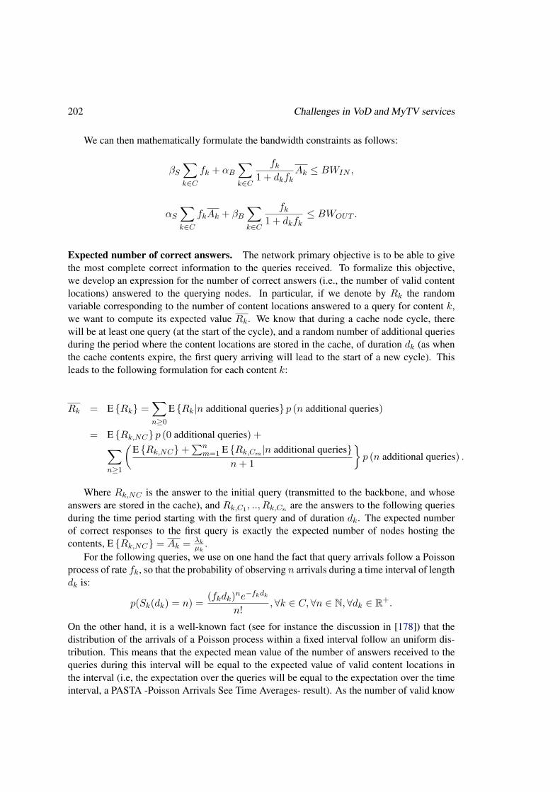
202 Challenges in VoD and MyTV services
We can then mathematically formulate the bandwidth constraints as follows:
βS∑k∈C
fk + αB∑k∈C
fk1 + dkfk
Ak ≤ BWIN ,
αS∑k∈C
fkAk + βB∑k∈C
fk1 + dkfk
≤ BWOUT .
Expected number of correct answers. The network primary objective is to be able to givethe most complete correct information to the queries received. To formalize this objective,we develop an expression for the number of correct answers (i.e., the number of valid contentlocations) answered to the querying nodes. In particular, if we denote by Rk the randomvariable corresponding to the number of content locations answered to a query for content k,we want to compute its expected value Rk. We know that during a cache node cycle, therewill be at least one query (at the start of the cycle), and a random number of additional queriesduring the period where the content locations are stored in the cache, of duration dk (as whenthe cache contents expire, the first query arriving will lead to the start of a new cycle). Thisleads to the following formulation for each content k:
Rk = E {Rk} =∑n≥0
E {Rk|n additional queries} p (n additional queries)
= E {Rk,NC} p (0 additional queries) +∑n≥1
(E {Rk,NC}+
∑nm=1 E {Rk,Cm |n additional queries}
n+ 1
}p (n additional queries) .
Where Rk,NC is the answer to the initial query (transmitted to the backbone, and whoseanswers are stored in the cache), and Rk,C1 , .., Rk,Cn are the answers to the following queriesduring the time period starting with the first query and of duration dk. The expected numberof correct responses to the first query is exactly the expected number of nodes hosting thecontents, E {Rk,NC} = Ak = λk
µk.
For the following queries, we use on one hand the fact that query arrivals follow a Poissonprocess of rate fk, so that the probability of observing n arrivals during a time interval of lengthdk is:
p(Sk(dk) = n) =(fkdk)ne−fkdk
n!, ∀k ∈ C,∀n ∈ N,∀dk ∈ R+.
On the other hand, it is a well-known fact (see for instance the discussion in [178]) that thedistribution of the arrivals of a Poisson process within a fixed interval follow an uniform dis-tribution. This means that the expected mean value of the number of answers received to thequeries during this interval will be equal to the expected value of valid content locations inthe interval (i.e, the expectation over the queries will be equal to the expectation over the timeinterval, a PASTA -Poisson Arrivals See Time Averages- result). As the number of valid know
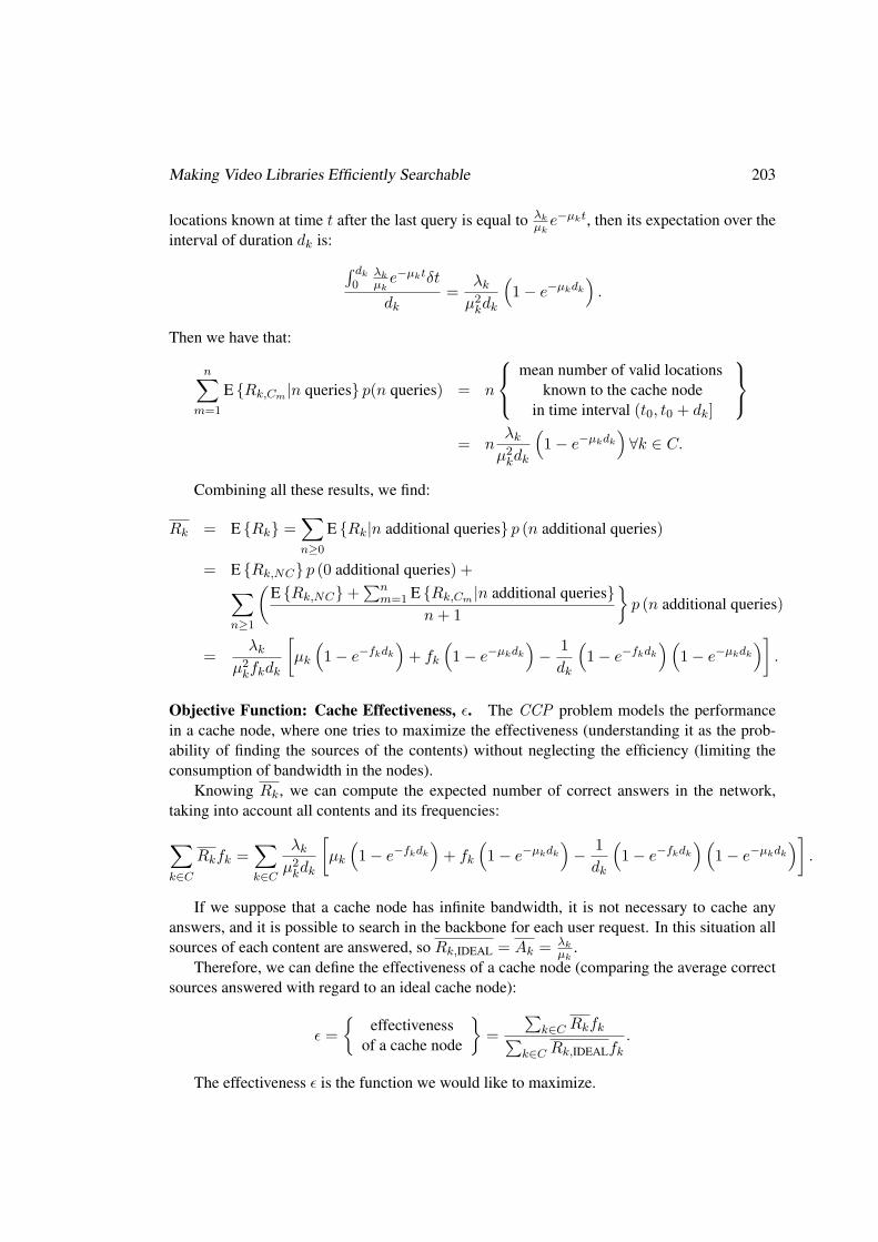
Making Video Libraries Efficiently Searchable 203
locations known at time t after the last query is equal to λkµke−µkt, then its expectation over the
interval of duration dk is: ∫ dk0
λkµke−µktδt
dk=
λkµ2kdk
(1− e−µkdk
).
Then we have that:
n∑m=1
E {Rk,Cm |n queries} p(n queries) = n
mean number of valid locations
known to the cache nodein time interval (t0, t0 + dk]
= n
λkµ2kdk
(1− e−µkdk
)∀k ∈ C.
Combining all these results, we find:
Rk = E {Rk} =∑n≥0
E {Rk|n additional queries} p (n additional queries)
= E {Rk,NC} p (0 additional queries) +∑n≥1
(E {Rk,NC}+
∑nm=1 E {Rk,Cm |n additional queries}
n+ 1
}p (n additional queries)
=λk
µ2kfkdk
[µk
(1− e−fkdk
)+ fk
(1− e−µkdk
)− 1dk
(1− e−fkdk
)(1− e−µkdk
)].
Objective Function: Cache Effectiveness, ε. The CCP problem models the performancein a cache node, where one tries to maximize the effectiveness (understanding it as the prob-ability of finding the sources of the contents) without neglecting the efficiency (limiting theconsumption of bandwidth in the nodes).
Knowing Rk, we can compute the expected number of correct answers in the network,taking into account all contents and its frequencies:∑k∈C
Rkfk =∑k∈C
λkµ2kdk
[µk
(1− e−fkdk
)+ fk
(1− e−µkdk
)− 1dk
(1− e−fkdk
)(1− e−µkdk
)].
If we suppose that a cache node has infinite bandwidth, it is not necessary to cache anyanswers, and it is possible to search in the backbone for each user request. In this situation allsources of each content are answered, so Rk,IDEAL = Ak = λk
µk.
Therefore, we can define the effectiveness of a cache node (comparing the average correctsources answered with regard to an ideal cache node):
ε ={
effectivenessof a cache node
}=
∑k∈C Rkfk∑
k∈C Rk,IDEALfk.
The effectiveness ε is the function we would like to maximize.

204 Challenges in VoD and MyTV services
maxdk∈R+
8><>:Pk∈C
λk
µ2kdk
hµk`1− e−fkdk
´+ fk
`1− e−µkdk
´− 1dk
`1− e−fkdk
´ `1− e−µkdk
´i.P
k∈C fkλkµk
9>=>;st:
βSXk∈C
fk + αBXk∈C
fk
1 + dkfk
λk
µk≤ BWIN // bandwidth capacity constraints
αSXk∈C
fkλk
µk+ βB
Xk∈C
fk
1 + dkfk≤ BWOUT // bandwidth capacity constraints
dk ∈ R+∀k ∈ C, //decision variables
fk, λk, µk ∈ R+∀k ∈ C
αS , αB , βS , βB , BWIN , BWOUT ∈ R+
Figure 11.6: CCP Mathematical Programming Model.
11.2.2 Mathematical programming formulation
If we put together the network objective and the bandwidth restrictions discussed in the previ-ous section, we arrive to the formulation of our CCP problem in Figure 11.6.
This is a non-linear optimization problem, both in the restrictions and in the objective func-tion. If we study it in detail, we can see that both the feasible solution space and the objectivefunction are convex. As the problem is stated as a maximization one, a convex objective func-tion will in general lead to multiple local optimum.
Content class based alternative formulation. In most cases, content networks manage avery large number of different contents. These means that the previous formulation will havea large class of decision variables dk, an additional difficulty for the numerical solution of theproblem. On the other hand, for simplicity design reasons, the networks will in general treat inthe same way contents that have similar characteristics. It is then possible to group all contentsin a certain number of content classes, such that all contents within a class have relativelyhomogeneous characteristics.
Formalizing, we suppose that all contents c ∈ C are grouped into K content classes, suchthat if two contents belong to the same class, all their parameters are identical:
C = C1 ∪ C2... ∪ CK
∀i, j ∈ Ck, ∀k ∈ [1..K]⇒
fi = fj ,λi = λj ,µi = µj
The size of class k, denoted by lk, is the number of contents of this class: ‖Ck‖ = lk∀k ∈[1..K]. The total number of contents in the network is then: ‖C‖ =
∑k∈K ‖Ck‖ =
∑k∈K lk.
We now define the Content Class Caching Problem (CCCP ). The problem is then formalizedin Figure 11.7.
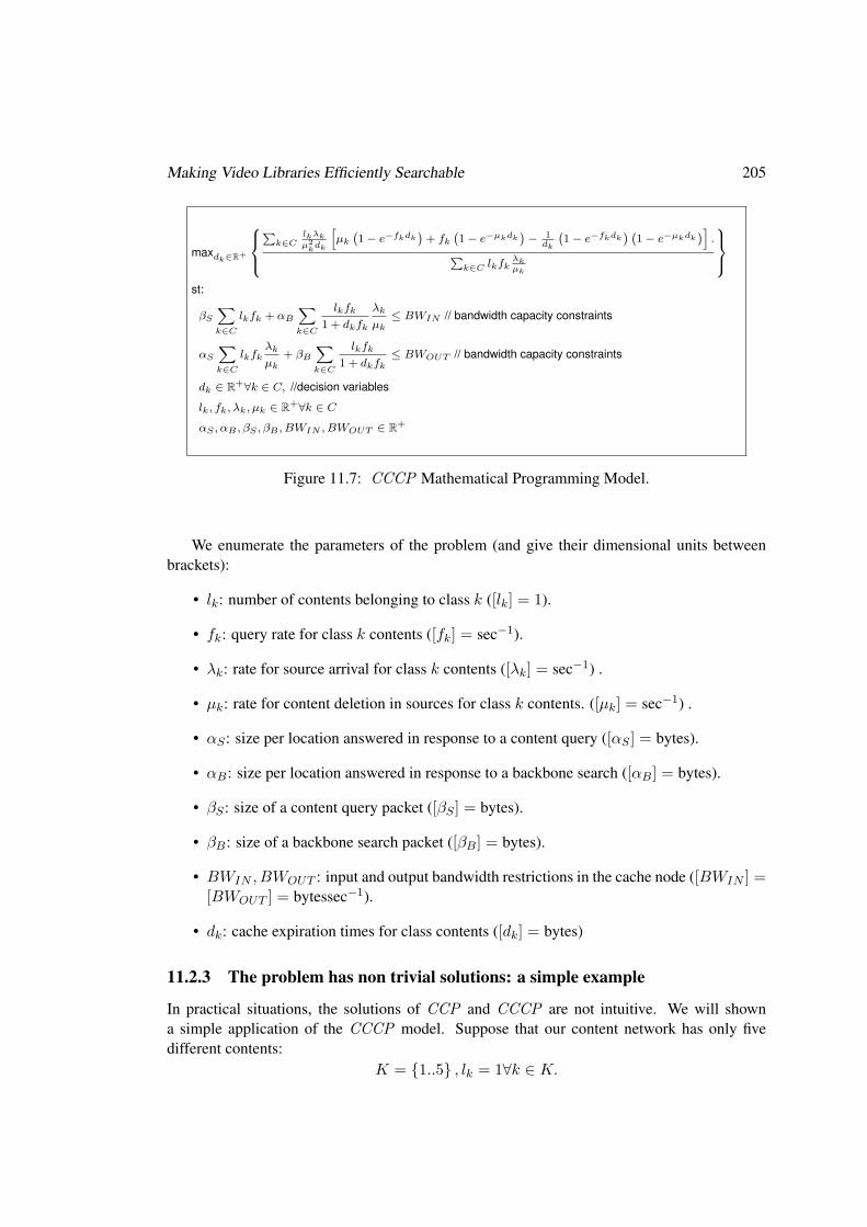
Making Video Libraries Efficiently Searchable 205
maxdk∈R+
8><>:Pk∈C
lkλk
µ2kdk
hµk`1− e−fkdk
´+ fk
`1− e−µkdk
´− 1dk
`1− e−fkdk
´ `1− e−µkdk
´i.P
k∈C lkfkλkµk
9>=>;st:
βSXk∈C
lkfk + αBXk∈C
lkfk
1 + dkfk
λk
µk≤ BWIN // bandwidth capacity constraints
αSXk∈C
lkfkλk
µk+ βB
Xk∈C
lkfk
1 + dkfk≤ BWOUT // bandwidth capacity constraints
dk ∈ R+∀k ∈ C, //decision variables
lk, fk, λk, µk ∈ R+∀k ∈ C
αS , αB , βS , βB , BWIN , BWOUT ∈ R+
Figure 11.7: CCCP Mathematical Programming Model.
We enumerate the parameters of the problem (and give their dimensional units betweenbrackets):
• lk: number of contents belonging to class k ([lk] = 1).
• fk: query rate for class k contents ([fk] = sec−1).
• λk: rate for source arrival for class k contents ([λk] = sec−1) .
• µk: rate for content deletion in sources for class k contents. ([µk] = sec−1) .
• αS : size per location answered in response to a content query ([αS ] = bytes).
• αB: size per location answered in response to a backbone search ([αB] = bytes).
• βS : size of a content query packet ([βS ] = bytes).
• βB: size of a backbone search packet ([βB] = bytes).
• BWIN , BWOUT : input and output bandwidth restrictions in the cache node ([BWIN ] =[BWOUT ] = bytessec−1).
• dk: cache expiration times for class contents ([dk] = bytes)
11.2.3 The problem has non trivial solutions: a simple example
In practical situations, the solutions of CCP and CCCP are not intuitive. We will showna simple application of the CCCP model. Suppose that our content network has only fivedifferent contents:
K = {1..5} , lk = 1∀k ∈ K.

206 Challenges in VoD and MyTV services
The content request frequency and the lodging rate are inversely proportional, see Ta-ble 11.1 for the detail of the description of the type of content that lodges the network. Usually,the backbone searches consume more bandwidth than the one needed for the clients, the Ta-ble 11.2 shows that a backbone search employs three times the bandwidth of a client request.
Table 11.1: Content lodged in the example network. Only five different contents, where thecontent request frequency and the lodging rate are inversely proportional.
k lk fk (1/s) λk (1/s) µk (1/s)1 1 0.01 100.00 12 1 0.10 10.00 13 1 1.00 1.00 14 1 10.00 0.10 15 1 100.00 0.01 1
Table 11.2: Communication in the example network. A backbone search needs three times thebandwidth of a client request.
βS (bytes) 1αS (bytes) 1βB (bytes) 3αB (bytes) 3
The problem only presents restrictions in the bandwidth consumption. It is expected that,if the bandwidth is wide enough then the cache node will not cache any request as a way tomaximize the correct answers. To see this effect in the solution we considered five differentavailable bandwidths, BWIN ∈ {112, 114, 117, 123, 127}. Table 11.3 shows the results foreach bandwidth restriction5.
It can be observed that the solution always reaches the maximum available bandwidthBWIN , except in the instance 5th, where it is possible not to cache the queries without ex-ceeding the available bandwidth. Since we expected, as more bandwidth is available bettersolutions are achieved: the efficiency changes from 20% (ε = 0.198563) to 100% (when thereis not caching) with regard to a network with perfect knowledge.
The solutions are less intuitive as the bandwidth is more restrictive. This simple exampleshows that, in general, not choosing a good caching policy can reduce drastically the efficiencyof a cache node. A common wrong assumption is that the best caching policy is to store themost requested content, another wrong possible policy it is do it with the least changeablecontent. For example, in the first instance (the one most compromised in available bandwidth)it is convenient to have larger expiration times in contents (Figure 11.8 following a compromisebetween popularity of a content and its lodging rate.
5As we will see later, the results are obtained using the AMPL [13] software with the MINOS [315] librarysolver.

Making Video Libraries Efficiently Searchable 207
Table 11.3: Results for the five instances, each ones with different bandwidth restriction.
Instance ε BWIN BWIN BWOUT dNormalized Available Input Output ExpirationObjective bandwidth bandwidth bandwidth Timefunction (bytes/hr) employed employed for each
(bytes/hr) (bytes/hr) content class1 0.198563 112 112 93.9766 1307750,
8639810,19096900,245619,
0.02371672 0.558249 114 114 60.3430 1075230,
8898270,0.798618,0.292056,0.0551847
3 0.834110 117 117 40.6829 69.0388,6.37234,1.16435,0.383453,0.0975636
4 0.997607 123 123 153.3330 0.105319,0.103796,0.092098,0.0564873,0.0137929
5 0.999999 127 126.1097 338.3000 0,0,0,0,0
1e-06
1e-04
0.01
1
100
10000
1e+06
1e+08
1 2 3 4 5
time
(sec
onds
)
content id
Cache Expiration Timeinstance 1instance 2instance 3instance 4instance 5
Figure 11.8: Expiration Times for the each instance, according to class of content.

208 Challenges in VoD and MyTV services
11.2.4 Relationship betwen CCP and CCCP models: symmetric solutions
Grouping the contents in classes allows to make the problem more treatable mathematically,because if the content is grouped in classes, then the number of variables (and the space offeasible solutions) diminishes drastically.
This implies that the CCCP presents as feasible solutions only those where the cacheapplies the same treatment to the contents with identical parameters: ∀i, j ∈ C\fi = fj , λi =λj , µi = µj ⇒ di = dj . Whereas in the generic CCP problem it is possible to find: i, j ∈C\fi = fj , λi = λj , µi = µj , di 6= dj .
This imposition of equity or symmetry in the solution of the CCCP problem implies thatsome good solutions of the generic problem are ignored. We show it in the following simpleexample.
11.2.4.1 An Example of Loss of Solutions.
Let’s suppose a network with two contents C = {c1, c2}, which belong to the same classK = {1}, with parameters: l1 = 2, f1 = λ1 = µ1 = 1, αS = αB = βS = βB = 1,BWIN ≥ BWOUT = 2.25.
Then, the CCP problem is defined as:
maxdk∈R+
{[1d1
(1−−e−d1)− 1
2d21
(1−−e−d1)2]+
[1d2
(1−−e−d2)− 1
2d22
(1−−e−d2)2]}
st:2 + 1
1+d1+ 1
1+d2≤ BWOUT , // bandwidth capacity constraints
d1, d2 ∈ R+ //decision variables
And the CCCP problem is defined as:
maxd1∈R+
{2d1
(1−−e−d1)− 1
d21
(1−−e−d1)2}
st:2 + 2
1+d1≤ BWOUT , // bandwidth capacity constrain
d1 ∈ R+ //decision variable
The objective function of the CCCP problem is decreasing monotonously, whereas thebandwidth restriction is increasing monotonously, therefore the optimal solution is reachedwhen the cache node is consuming its maximum available bandwidth: d1 = 7 and ε =0.265083. On the other hand, the CCP problem presents better performance if asymmetricsolutions are considered, for example: d1 = 3.4032, d2 = 42.6857 and ε = 0.266874.
11.2.5 Compromise between Publication and Search
In the chapter introduction (Section 11.1.2) we present the compromise between publicationand search. In the cache nodes, this commitment is expressed by the time that the query an-swers are stored; i.e. the time of caching for any content k, called dk. Querying nodes areconnected to at least one aggregation node in order to route their queries. The aggregationnode concentrates all queries of its connected nodes and consults the backbone when it is not

Making Video Libraries Efficiently Searchable 209
able to directly answer the queries with its cache of the results of recent queries (i.e. expirationtime of this content). The previous results of a content k are systematically deleted after aperiod dk, because the nodes which publish this content can disconnect or delete it. Therefore,the optimal expiration time dk depends of the dynamics in the lodged content process and thequery frequency. If the lodgment of a content k is very dynamic, it will be expected that itwill not be efficient to cache the answers (because they become out dated quickly), this impliesa lower dk. In the opposite situation, when a content is heavily queried, it will be expectedthat its queries will be cached a longer time (i.e. a high dk). This is the compromise betweenpublication and search, and we will show it in our CCP model.
High expiration time: If the expiration time dk of a content grows, then the average numberof correct answers diminishes to the point of which the cache node does not return any validanswer: lim
dk→+∞Rk = 0 ∀k ∈ C.
Therefore, if an infinite expiration time is supposed for all the contents, the cache nodedoes not answer correctly any valid location, using a minimal bandwidth:
limdk→+∞
ε = infdk∈R+
{ε} = 0 ∀k ∈ C
limdk→+∞
{bandwidth in} = infdk∈R+
{bandwidth in} = βS∑k∈C
fk ∀k ∈ C
limdk→+∞
{bandwidth out} = infdk∈R+
{bandwidth out} = αS∑k∈C
fkAk ∀k ∈ C
Low expiration time: On the other hand, if the expiration time dk of a content diminishesto very low values, the cache node answers perfectly all the requests (i.e. it answers all thesources that lodges the content): lim
dk→0+Rk = Ak = λk
µk∀k ∈ C.
Therefore, with an instantaneous expiration time for all the contents, the cache node an-swers perfectly all the valid content locations, using the maximum available bandwidth:
limdk→0+
ε = supdk∈R+
{ε} = 1 ∀k ∈ C
limdk→0+
{bandwidth in} = supdk∈R+
{bandwidth in} = βS∑k∈C
fk + αB∑k∈C
fkAk ∀k ∈ C
limdk→0+
{bandwidth out} = supdk∈R+
{bandwidth out} = αS∑k∈C
fkAk + βB∑k∈C
fk ∀k ∈ C
According to the dynamism that presents the content locations in the sources (expressed byλk and µk in our model) and the frequency of requests (fk) we fix the optimal expiration time(dk) in the cache node, restricted by the available bandwidth.
The same conclusions can be applied to the CCCP model.

210 Challenges in VoD and MyTV services
11.3 On the Application of the Efficient Search
11.3.1 Content Networks
The Content Class Caching Problem (CCCP ) (presented on previous section 11.2) can be ap-plied to a wide range of Content Networks. In our previous work [274, 276, 277, 279] wepresent a taxonomy of Content Networks, based on their architectures. Some of the character-istics studied were the decentralization of the network, the content aggregation and the contentplacement. Also we analyze their behaviors, in terms of performance and scalability. Depend-ing on the specific application of the content network, and mainly depending on the content dy-namics in the network, different architectures design are used. Actually, the presence of cachenodes in content networks is apparently mandatory because of scalability reasons. Figure 11.9shows a simplified view of well know content networks. New file-sharing P2P networks havecache nodes to improve their searching performance. In unstructured P2P networks with a hi-erarchical decentralization, usually the most compromised nodes have query caching facilities.For instance, eMule [89] (Figure 11.9(a)) has dedicated servers (typically with the Lugdunumsoftware), which concentrate the queries of any peer connected to them. In eMule, each peerconnects to a unique server, who will propagates the peer’ queries in the network and returnthe consolidated answers to the peer. In KaZaA [190] (Figure 11.9(b)), the concept is identical,with the expection that the servers are also peers, called superpeers. For redundancy reasons, inKaZaA, each peer connects in average to three superpeers simultaneously (for simplification,not shown in the figure). Hybrid P2P systems, like Napster [230] (Figure 11.9(c)), does notneed the query caching facility, because the central server has a global view of the content inthe network. In pure peer-to-peer networks, like Gnutella [115] (Figure 11.9(d)) and Freenet,there are no cache node because all nodes have equal roles. Some P2P protocols, for exampleBitTorrent [30], does not provide a mechanism for content discovery, and therefore no querycaching is done (in these networks, the content discovery is done outside the network, typicallyin the Web). The cache nodes are not used exclusively in peer-to-peer networks, for instance,they are present in the Domain Name System (DNS) [39, 143, 144, 242] (Figure 11.9(e)),where they are called recursive servers. Next we will present other work related to our CCCPmodel.
11.3.2 Other Approaches: Expiration Time in Cache Nodes
There are a lot of works related to the estimation of expiration times in the cache nodes ofa content network. In general their objectives are to reduce the latency and the traffic in thedelivery of the content to the final user. In this section we summarize the work related in thisaspect.
First, it is important to highlight that the cache technology comes out its application of thecontent networks. It is used for the memory access and disc access in the computers [22, 337],in the file systems (distributed or not) [5, 76, 232], in the routing protocols, in the distributeddatabases [241, 301], in mobile networks [44, 61], in the content networks (for the queries [29,205, 208, 212, 297] or in the information lodging [95, 114, 132]), etc. According to eachapplication, different models and technologies have been developed, we summarize in thissection those ones related to content networks.

On the Application of the Efficient Search 211
(a) eMule. (b) KazAa.
(c) Napster. (d) Gnutella.
(e) DNS.
Figure 11.9: Simplified view of well know content networks.
212 Challenges in VoD and MyTV services
11.3.2.1 Consistency of the Information.
In many content networks the information consistency is crucial. In the cache nodes the incon-sistency happens when they answer an invalid information, because the source has deleted thecontent (or has disconnected).
For example, in the DNS system it is extremely important to assure that the answers to themapping among domain names and IPs should be correct, in another case there would arisesome problems of safety (we will see later on that actually the DNS does not have the wholeconsistency wished).
11.3.2.2 Time-to-Live (TTL) Method.
When the information consistency is necessary, the network designer must include in the pro-tocols some mechanisms to ensure it. If there are cache nodes, then the most used method isthe TTL (time to live).
Each content is published by the sources with an associated time to live, the TTL. TheTTL determines the maximum time in which a source assures that the content is going toremain unchanged and therefore it is the maximum expiration time allowed in the caches. Inthe first request of a content, the cache node obtains the answer of some source together with aTTL, for the following queries included in the interval TTL the cache can answer this sourcewithout consulting it again, after this period the cache node must erase the content of the cacheand consult to the source again for the content.
Several networks use TTL’s method, for example the World Wide Web and the DNS sys-tem. The cache nodes in the Web they are known as proxies Web, whereas in the DNS’snetwork are known as recursive servers.
World Wide Web - Proxies Web. Most of the effort made in related works is in the study ofthe proxies cache for the WWW [4, 38, 53, 62, 65, 66, 124, 195–197, 217, 307, 340, 348, 350].The TTL mechanism assures partially the information consistency in the HTTP caches, ingeneral the previous studies on this topic are in two possible directions:
• To choose efficiently the contents to lodge in the cache, supposing a restriction in capac-ity, and
• to define policies (or algorithms) to lodge efficiently the contents (for example to choosethe expiration times).
With respect to the contents to lodge in the cache, several techniques of prefetching havebeen proposed and proved [65, 66, 124, 340, 348, 350].
With respect to the policies definition, there are several works that test in a simulationcontext or with real data different algorithms. Some of these works are similar to our approachbecause they present optimization models who consider the dynamics of the content in thesources:
• Xing Y., in his MSc. work “Caching on the Changing Web” [355] presents an opti-mization model of the cache on proxies Web. The function to maximize is the benefit
On the Application of the Efficient Search 213
achieved by the decrease of latency in the final users and the cost is the space of availablelodging in the cache. In his analysis, he classifies the contents in four classes dependingon the request frequency and the lodging ratio.
• Gopalan P. et. al. in the work “Caching with Expiration Times” [117] show that somecomplex policies do not differ in performance with regard to other simple policies.
• Shim J. et. al. [307]. Their approach is very similar to Xing’s work , they do not dividethe contents in classes and they study other algorithms for the cache policies.
• Krishnamurthy B. et. al. [195–197] analyze different algorithms to estimate the expira-tion time in the caches depending on the query rate.
• Chen X. et. al. [53] study the expiration time of Web content. They classify the contentsin four classes also; and they present a new algorithm to the expiration policy.
Domain Name System - Recursive servers. In spite of its importance, there are not so manyworks that study the cache performance in a recursive server. The caching policy must differfrom other content networks (as the World Wide Web) given the nature of the content that islodged:
• the contents have very small size and it is not a problem to lodge them;
• the search in the backbone (when the answer is not cached) cache has a high cost oflatency in comparison to other systems;
• the expiration time is much less than the time between changes in the content;
• the content is generally lodged in redundant sources, and the access time differs amongthe sources;
• there are many authoritative servers badly configured (for example with LAME delega-tions), causing excessive delays in the search with time-out’s.
The recursive servers incorporate a passive policy in the cache managing. The content isstored exclusively after a query node requests it, and is stored strictly according to the TTLoffered by the source. Studies on this topic analyze improvements in different aspects 6:
• to define policies (or algorithms) to lodge efficiently the contents (in some cases: tochoose the expiration time);
• and to correlate the searches in DNS to the use of other networks (specially the WWW).
Most of the works tackle the definition of policies to store efficiently the queries in therecursive servers. E. Cohen and H. Kaplan seem to be very active in this area, developingstudies in the DNS system [64] and in the World Wide Web [62, 63, 66]. The first improvement
6Since the small size that has the content in the DNS network, it is not necessary to choose efficiently whichcontent will be stored in the cache, like the studies in WWW.
214 Challenges in VoD and MyTV services
that appears is the pre-fetching search (or renovation policy): for very requested contents thecontents of the cache refresh themselves generating unrequested searches, this eliminates thelatency in the first resolution of a content.
Other improvements are done in the manipulation (in general the reduction) of the TTLstored in the cache. J. Jung et. al. model the behavior of the TTL mechanism [188] andits application to define policies on the DNS cache [189]. In general, the conclusion of theirstudies is that the influence of the policies of TTL managing are minimal and has no impact inthe speed of navigation perceived by the final users [310].
Some authors discuss the utilization of joint policies between the World Wide Web and theDNS, to reduce the latency perceived by the final users. The underlying idea is to look for thecooperation and synchronism between DNS’s caches and Web navigation. The pre-fetchingneeds predictive information on the future behavior of the query nodes. In general the cachesuse statistical information, supposing regularity among users (for example it is supposed thata content very requested previously will be very requested in the future). Nevertheless moreknowledge on the applications that generate the queries in DNS provides a more refined predic-tion. A. S. Hughes and J. Touch study the traces of a proxy Web to predict the future navigationsof the clients and they use this information to pre-fetch in the DNS [138, 139]. E. Cohen andH. Kaplan also study this idea, they analyze the pre-resolution of names [65], and also theystudy the simultaneous validation between the Web content and the DNS answers, achievinggood results in small environments, when there are slow dynamics in the DNS sources [64].
On The strict Use of TTL In most of the networks that implement TTL mechanism, theTTL is not respected strictly. The clients of a network that offers a TTL mechanism often donot respect the cache time and keep the information as valid after its TTL expired. This be-havior introduces serious disadvantages from the point of view of the manager of the network,but some advantages from the point of view of the final user: a strictly use of the TTL times isa restriction on the generic problem of diminishing the delays and the traffic in the delivery ofthe content to the final user, specially when there are slow dynamics in the content changes.
For example in the World Wide Web, all the Internet browsers (Microsoft Internet Ex-plorer7, Mozilla-Netscape8 , etc.) do not respect the expiration time received in every HTTPconnection.
These products are in competition to offer the most quick browsing experience, this isincompatible with a strict use of the standard in respect to the TTL, because it would generatemore requests to the sources and therefore more delay in the display of the web pages. Theproblem arises in the fact that the TTL offered by the sources rarely imply a change in thecontent. If whenever the TTL is expired the source makes a change in the content unfailinglythe Web browsers should respect the standard because in another case they will display wronginformation, something that the users would perceive wrongly.
From the content sources point of view, in general they can not anticipate when they will up-date their contents, therefore the common behavior is to use the average time between changesfor the TTL. This limitation is so clear that we do not know Web server implementations, or
7Internet Explorer. Home Page. http://www.microsoft.com/windows/ie/8Mozilla Home Page. http://www.mozilla.org/
On the Application of the Efficient Search 215
DNS authoritative server implementations, that can schedule future changes and reduce gradu-ally the TTL to exactly inform to the cache nodes of the next change. Only few administratorsof these systems know this level of detail and therefore in general the default TTL is used.Therefore, in practice, the TTL does not specify the minimal time of unchanged content, it justreports the average time between changes.
The recursive servers implementations and proxies Web implementations that belong to thepublic domain use the TTL mechanism strictly (for example BIND [229] and Squid [313]),nevertheless some proprietary implementations do not use it arguing improvements in the per-formance.
11.3.2.3 Other networks and methods - Peer-to-Peer networks.
The P2P file sharing networks do not use the TTL’s mechanism, and its application would beinefficient because the indeterminate dynamism in the lodged content.
Some applications use a P2P infrastructure to offer a decentralized and anonymous proxyWeb (for example Squirrel [179] that uses Pastry [287] as network infrastructure).
The P2P traffic represents an important percentage of the bandwidth consumption in theinternational links of every ISP. These links in general are costly and the growth in their usageis a worry for the ISP.
Several companies offer equipment that guarantees a reduction of the bandwidth consump-tion in the international links due to P2P applications. This equipment stores and guides thetraffic of the most popular P2P applications in order to use efficiently the link. These equip-ments are cache nodes in these networks, with a particular policy in respect to the expirationtime of contents out side the ISP network. Examples of these equipments are: PacketShaper9,Peer-to-Peer-Element10 and PeerCache11.
11.3.2.4 CCP , CCCP models and the TTL mechanism.
The CCP and CCCP models presented in this chapter do not contemplate the TTL mecha-nism that several content networks include to preserve the information consistency. The TTLcan be added to the CCP problem directly if we add the restriction in the expiration time ofevery content. The same directly extension is possible in the CCCP problem, where everycontent in a class has the same TTL. It is potentially a very strong restriction, because theTTL of a class has to be the minimal TTL among the contents of the class. Therefore, in thiscase it is necessary to study in depth the impact of the TTL restriction on the solution.
It is necessary a comparative study of the the information consistency between the currentnetworks with TTL and those who arise of the use of the CCP and CCCP models.
In the following section, we apply the models to two real network cases: a file sharingP2P network (without TTL’s mechanism), and a DNS recursive server (that includes TTL).We expect a similar behavior in the workload of the P2P network with respect to the Video on
9Packeteer’s PacketShaper® Home Page http://www.packeteer.com/products/packetshaper.cfm.10Sandvine Incorporated. Home Page. http://www.sandvine.com/.11PeerCache de Joltid. Home Page. http://www.joltid.com/index.php/peercache.

216 Challenges in VoD and MyTV services
Demand service of our GOL!P2P prototype. Also we expect a similar behavior between theDNS study and the MyTV service.
11.4 Estimate the Performance Using “Similar” Real Data
11.4.1 Caching VoD searches
In this section we present a numerical illustration of the CCCP approach over a case study,where the data was generated with information available in different literature sources espe-cially referring to Gnutella or similar peer-to-peer (P2P) file sharing networks [57, 123, 211,300, 359]. We have chosen file-sharing P2P networks, because we expect similar user behaviorfor the VoD service, and also because there is also much quantitative information available forP2P networks.
Table 11.4: Parameter values for a file sharing case study (a similar behavior is expected inVoD).
Parameter ValueT : time units 1 hourC: number of different contents 878691f : average content query rate 0.037938251 hr-1fmax: maximum content query rate 1000 hr-1λ: average content storage rate 11.09749966 hr-1µ: average content location validity rate 1 hr-1“λµ
”max
: maximum allowed number of locations
answered in response to a content query 200αS : size of a the answer to a content query 100 bytesαB : size of the answer of a backbone search 310 bytesβS : size of a content query 94 bytesβB : size of a backbone search packet 291.4 bytesBWIN : input bandwidth 921600000 bytes/hr.BWOUT : output bandwidth 460800000 bytes/hr.
Table 11.4 summarizes the main parameters of the case study. We generated ten CCP in-stances of this detailed case study (using a random number generator with different seeds), in-cluding the data for the 878691 different contents (which correspond to the number of Gnutellacontents in the study by Chu [57]), where the distributions for the query frequency follow amodified Pareto distribution law taking into account the "fetch-at-most-once" effect (see [123]for a discussion of this observed network behavior). Regarding the frequency of arrival of newstorage locations for each content, we suppose that it is linearly related to the query frequency,following the hypothesis mostly used in the literature (an exception is the work by Qin [211]which also studies a square root dependency). For the bandwidth constraints, we suppose thatthe cache nodes will be equipped with an ADSL 2/1 Mbps connection as reference value. Theaverage packet sizes in Gnutella was measured by Yang [359].

Estimate the Performance Using “Similar” Real Data 217
11.4.1.1 Number of content classes in the CCCP .
As we discussed in section 11.2.2, it is next to impossible to directly solve the CCP problemgenerated, a non-linear problem in 878691 independent variables (one for each content). Asan alternative, we cluster the contents into a small number of homogeneous content classes,and solve the resulting CCCP problem. As it is not a-priori clear what is the best number ofclasses to use, we experimented with five different values, namely 2, 8, 16, 32, and 128 classes,for each of the ten different CCP problems generated.
The problem was programmed using the AMPL modeling language; AMPL [13, 263] isa software with a algebraic modelling language for doing mathematical programming, whichcan be used to easily represent a non-linear mathematical programming problem such as theCCCP . We solved the problem using AMPL in conjunction with MINOS [226, 315] (version5.5), an optimization solver12.
All experiments were run on a PIII 800 MHz computer, with 320 Mb RAM space. Theten instances results obtained per class are averaged in Table 11.5. Among other observations,we can see that when the number of classes grow, the available resources (i.e. the BWOUT
employed) are being increasingly used. Also, the computational times required to solve themodel grow, albeit they remain very modest.
Table 11.5: Average results for 10 (randomly generated) cases of a file sharing case study (asimilar behavior is expected in VoD).
Number Normalized Execution Input Outputof content Objective time bandwidth bandwidth
classes function ε (secs.) employed employed(bytes/hr) (bytes/hr)
2 0.99888275 0.00625 921599933 3341573258 0.98845330 0.07400 921599993 40628213816 0.98759660 0.25800 921599993 41349085132 0.99659690 0.21100 921599993 415901600
128 0.99924110 0.44900 921600793 416588930
As in CCCP we are dealing with aggregated data, For comparing reasons, it is importantto translate back the results into the terms of the original CCP problem. In particular, we nowconsider again the 878691 different contents, and we evaluate the number of correct answers toqueries if we use for each content the cache expiration times given by the optimization models.Table 11.6 summarizes this comparison. From this table, we can see that if the number ofclasses is too low, then the approximation error incurred in the aggregated model is very large,and the percentage of correct answers to queries in the real problem will be much below thenominal values computed by the optimization procedure. This discrepancy gets very quicklyirrelevant when the number of classes increase, when we have 128 classes the results coincide.
Each content network has its own profile in respect to the query frequency and store dy-namics. This profile influences on the degree of similarity of the contents in the network, fromour model point of view, and therefore how many CCCP classes are needed to compute with anegligible approximation error. In the P2P instances evaluated, with 32 classes or 128 classes,
12Other optimization solvers were tested, see [274] for details.
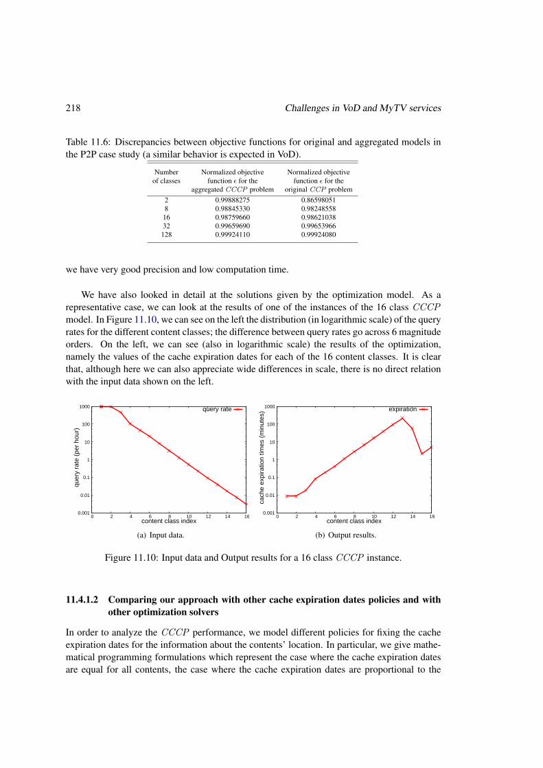
218 Challenges in VoD and MyTV services
Table 11.6: Discrepancies between objective functions for original and aggregated models inthe P2P case study (a similar behavior is expected in VoD).
Number Normalized objective Normalized objectiveof classes function ε for the function ε for the
aggregated CCCP problem original CCP problem2 0.99888275 0.865980518 0.98845330 0.98248558
16 0.98759660 0.9862103832 0.99659690 0.99653966128 0.99924110 0.99924080
we have very good precision and low computation time.
We have also looked in detail at the solutions given by the optimization model. As arepresentative case, we can look at the results of one of the instances of the 16 class CCCPmodel. In Figure 11.10, we can see on the left the distribution (in logarithmic scale) of the queryrates for the different content classes; the difference between query rates go across 6 magnitudeorders. On the left, we can see (also in logarithmic scale) the results of the optimization,namely the values of the cache expiration dates for each of the 16 content classes. It is clearthat, although here we can also appreciate wide differences in scale, there is no direct relationwith the input data shown on the left.
0.001
0.01
0.1
1
10
100
1000
0 2 4 6 8 10 12 14 16
quer
y ra
te (
per
hour
)
content class index
query rate
(a) Input data.
0.001
0.01
0.1
1
10
100
1000
0 2 4 6 8 10 12 14 16
cach
e ex
pira
tion
times
(m
inut
es)
content class index
expiration
(b) Output results.
Figure 11.10: Input data and Output results for a 16 class CCCP instance.
11.4.1.2 Comparing our approach with other cache expiration dates policies and withother optimization solvers
In order to analyze the CCCP performance, we model different policies for fixing the cacheexpiration dates for the information about the contents’ location. In particular, we give mathe-matical programming formulations which represent the case where the cache expiration datesare equal for all contents, the case where the cache expiration dates are proportional to the

Estimate the Performance Using “Similar” Real Data 219
maxd∈R+
8<:Pk∈C
lkλk
µ2kd
ˆµk`1− e−fkd
´+ fk
`1− e−µkd
´− 1d
`1− e−fkd
´ `1− e−µkd
´˜.P
k∈C lkfkλkµk
9=;st:
βSXk∈C
lkfk + αBXk∈C
lkfk
1 + dfk
λk
µk≤ BWIN // bandwidth capacity constraints
αSXk∈C
lkfkλk
µk+ βB
Xk∈C
lkfk
1 + dfk≤ BWOUT // bandwidth capacity constraints
d ∈ R+∀k ∈ C, //decision variable
lk, fk, λk, µk ∈ R+∀k ∈ C
αS , αB , βS , βB , BWIN , BWOUT ∈ R+
Figure 11.11: SETP Mathematical Programming Model.
query frequency for a content, and the case where all cache expiration dates can be fixed inde-pendently, i.e. the CCCP .
Policies for fixing Cache expiration dates. Based on the previous model, we now discussthree alternative ways to fix the cache expiration dates.
• Single expiration time policy (SETP). The simplest option for solving the problem issetting the same expiration time for all contents. In this case, the aggregation node de-fines a fixed expiration time d; for every content location query, the information is storedin the cache during this time, and then deleted. This amounts to having all variablesdk = d in the previous formula, leading to the mathematical programming formulationin Figure 11.11.
• Expiration time proportional to query rates policy (PETP). The query rate has animportant impact in the behavior of the different contents. It can be reasonable to assumethat high query rates correspond to contents with high impact and that their expirationtimes must then be kept longer; the easiest way is to impose a linear dependency. In thiscase, there is a single coefficient e such that for every content k, dk = efk . Then, themathematical programming formulation is shown in Figure 11.12.
• Optimal policy (CCCP ). If all values dk are free, unrelated variables, solving the op-timization model will give the theoretical optimum for the cache expiration policy prob-lem. The CCCP formulation is then the most general one.
The three problems are non-linear optimization problems, both in the restrictions and in theobjective function. We can see that both the feasible solution space and the objective functionare convex. As the problem is stated as a maximization one, a convex objective function willin general lead to multiple local optimum.

220 Challenges in VoD and MyTV services
maxe∈R+
8><>:Pk∈C
lkλk
eµ2kfk
hµk
“1− e−ef
2k
”+ fk
`1− e−eµkfk
´− 1efk
“1− e−ef
2k
” `1− e−eµkfk
´i.P
k∈C lkfkλkµk
9>=>;st:
βSXk∈C
lkfk + αBXk∈C
lkfk
1 + ef2k
λk
µk≤ BWIN // bandwidth capacity constraints
αSXk∈C
lkfkλk
µk+ βB
Xk∈C
lkfk
1 + ef2k
≤ BWOUT // bandwidth capacity constraints
e ∈ R+∀k ∈ C, //decision variable
lk, fk, λk, µk ∈ R+∀k ∈ C
αS , αB , βS , βB , BWIN , BWOUT ∈ R+
Figure 11.12: PETP Mathematical Programming Model.
Numerical Illustration. In this section we present a numerical illustration over a case study.The instance we discuss here was generated using the parameters of the Table 11.4. We solvedthe three different problems formulated using AMPL software with the different solvers avail-able at NEOS [73, 122]. The particular optimization solver used are MINOS, IPOPT [165],KNITRO [365], LANCELOT [201], PENNON [254], and SNOPT [315]. The better perfor-mance was achieved using the SNOPT solver.
We compare the three optimization policies above described. As the full problem generatedhas a large number of contents (878691), we used the 16 content classes instance, and we solvethis reduced problem. The results are then cast back in terms of the original problem13.
Table 11.7: Problem solutions, for 16 content classes instance, with the three policies: CCCP ,SETP and PETP .
CCCP SETP PETPOptimization Objective Execution Objective Execution Objective ExecutionSolver Function ε Time (s) Function ε Time (s) Function ε Time (s)MINOS 0.99610320 0.520 0.99995210 0.020 0.99993000 0.020IPOPT 0.99995470 0.030 0.99995210 0.040 0.99992800 0.040KNITRO 0.99995310 0.640 0.99995190 0.140 0.99658890 0.050LANCELOT 0.99975880 0.180 0.99995210 0.010 0.01368548 0.030PENNON 0.99955790 0.130 0.99995210 0.030 0.99993000 0.030SNOPT 0.99995470 0.010 0.99995210 0.030 0.99993000 0.030
Table 11.7 shows the objective values and the computing times for the three policies, inthe 16 class problem. The execution times are short, even if it can be seen that the CCCPpolicy takes longest to compute to optimality. Table 11.8 shows the objective function values,as computed in the original CCP case. As expected, it can be seen that the CCCP policy
13The original CCP problem could not be solved directly on NEOS due to its file size limitations in the usedoptimization interfaces.

Estimate the Performance Using “Similar” Real Data 221
Table 11.8: Solutions transformed to the original problem. For the policies: CCCP , SETPand PETP .
CCCP SETP PETPOptimization Aggregated Original Aggregated Original Aggregated OriginalSolver Objective Objective Objective Objective Objective Objective
Function ε Function ε Function ε Function ε Function ε Function εMINOS 0.99610320 0.99553881 0.99995210 0.99995200 0.99993000 0.99993040IPOPT 0.99995470 0.99995404 0.99995210 0.99995200 0.99992800 0.99992847KNITRO 0.99995310 0.99995215 0.99995190 0.99995174 0.99658890 0.99661043LANCELOT 0.99975880 0.99974659 0.99995210 0.99995200 0.01368548 0.01393887PENNON 0.99955790 0.99953126 0.99995210 0.99995199 0.99993000 0.99993039SNOPT 0.99995470 0.99995405 0.99995210 0.99995200 0.99993000 0.99993040
obtained the best results, with ε = 0.99995405 for the original problem. All the same, theother policies resulted in values not far away from this optimum.
11.4.2 Caching MyTV searches
In order to apply our framework to the MyTV service, it is necessary to obtain from measure-ments or previous studies the information about the parameters of the class contents. For it,we look at the DNS (Domain Name System) [39, 143, 144, 242], which is the system used onInternet in order to map symbolic domain names (such as www.fing.edu.uy) into IP addressescorresponding to actual computers in the network (such as 164.73.32.3). We expect a similarbehavior in the query frequency of the DNS and the MyTV service. The network actually mod-eled corresponds to the .uy (Uruguay) subdomain of Internet, and the parameters used are basedon real data obtained thanks to the support of ANTEL14, which is a state-owned company, andthe largest telco in Uruguay.
11.4.2.1 Parameters for the DNS network.
DNS (Domain Name System) can be seen as a content network with hierarchical distribution,where the information consistency is one of the most important objectives. DNS is basedon a network of recursive servers, which pass on queries until finding authoritative answers,which minimize the probability of information inconsistency (even if the correctness cannot becompletely guaranteed). In our case, we are interested in recursive servers, which correspondto the aggregation nodes of our general model. We collected real data from the recursiveservers at ANTEL, which daily serve hundreds of thousands users, with daily peak query ratesof approximately 1800 queries per second. The parameters of the model are summarized inTable 11.9.
As previously discussed, in our study we only took into account the behavior of the Uruguayandomains, i.e., those whose names finish by .uy. We collected ten consecutive days of recursiveserver logs, in order to estimate the total number of contents and the distribution of query rates.ANTEL DNS infrastructure employs the BIND software15, which was very useful as the logs
14ANTEL - Administración Nacional de Telecomunicaciones, http://www.antel.com.uy.15Berkeley Internet name domain, by Internet Software Consortium, http://www.isc.org/products/BIND.

222 Challenges in VoD and MyTV services
Table 11.9: Parameter values for a domain name system case study (a similar behavior isexpected in MyTV).
Parameter ValueC: number of different contents 220107f : average content query rate Empirical distribution
(heavy tailed, see Figure 11.13)λ: average content storage rate 0.8361 hr-1µ: average content location validity rate 0.5158hr-1αS : size of a the answer to a content query 169.6 bytesαB : size of the answer of a backbone search 1150.3 bytesβS : size of a content query 80.45 bytesβB : size of a backbone search packet 385.6 bytesBWIN : input bandwidth 1.933× 108 bytes/hr.BWOUT : output bandwidth 3.445× 108 bytes/hr.
1
10
100
1000
10000
100000
1e+06
0 10000 20000 30000 40000 50000 60000 70000
quer
y fr
eque
ncy
content identification
query frequency
Figure 11.13: Domain query rates distribution (tail cut off).
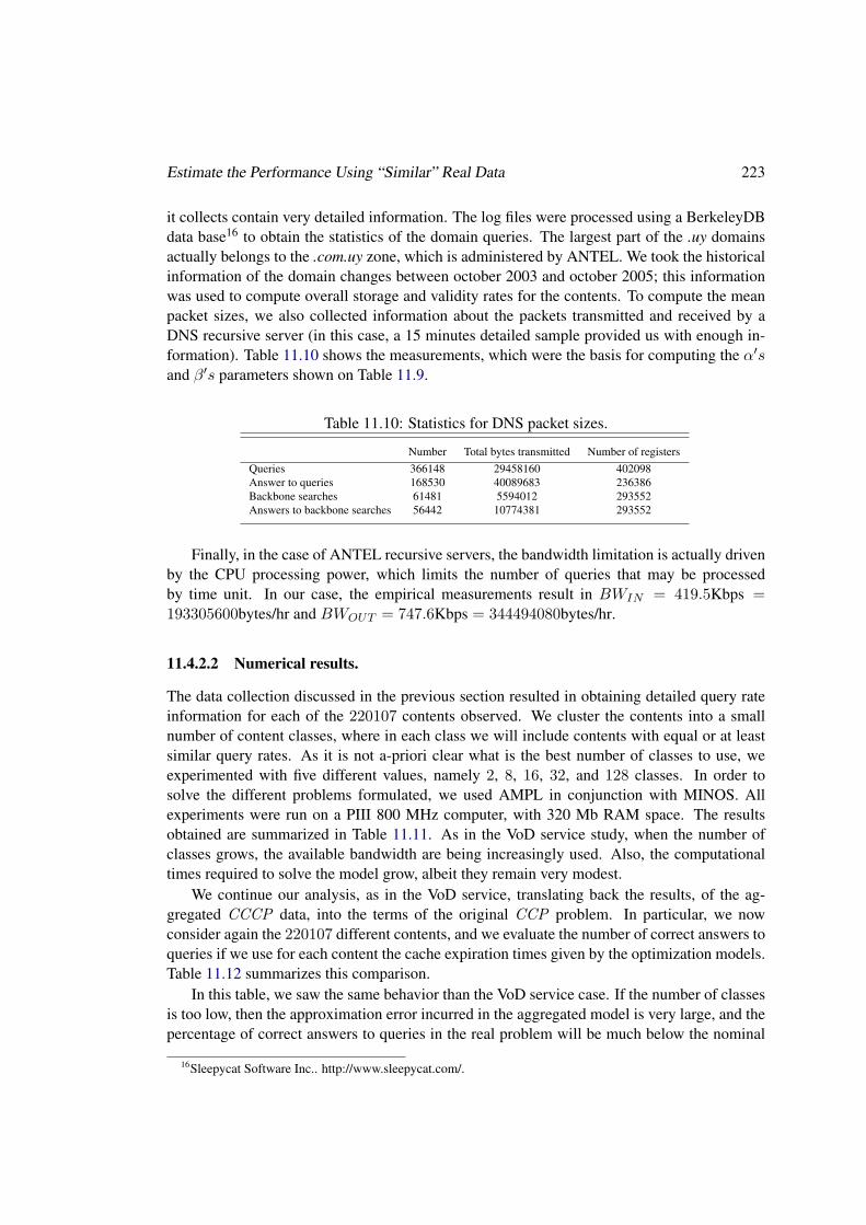
Estimate the Performance Using “Similar” Real Data 223
it collects contain very detailed information. The log files were processed using a BerkeleyDBdata base16 to obtain the statistics of the domain queries. The largest part of the .uy domainsactually belongs to the .com.uy zone, which is administered by ANTEL. We took the historicalinformation of the domain changes between october 2003 and october 2005; this informationwas used to compute overall storage and validity rates for the contents. To compute the meanpacket sizes, we also collected information about the packets transmitted and received by aDNS recursive server (in this case, a 15 minutes detailed sample provided us with enough in-formation). Table 11.10 shows the measurements, which were the basis for computing the α′sand β′s parameters shown on Table 11.9.
Table 11.10: Statistics for DNS packet sizes.
Number Total bytes transmitted Number of registersQueries 366148 29458160 402098Answer to queries 168530 40089683 236386Backbone searches 61481 5594012 293552Answers to backbone searches 56442 10774381 293552
Finally, in the case of ANTEL recursive servers, the bandwidth limitation is actually drivenby the CPU processing power, which limits the number of queries that may be processedby time unit. In our case, the empirical measurements result in BWIN = 419.5Kbps =193305600bytes/hr and BWOUT = 747.6Kbps = 344494080bytes/hr.
11.4.2.2 Numerical results.
The data collection discussed in the previous section resulted in obtaining detailed query rateinformation for each of the 220107 contents observed. We cluster the contents into a smallnumber of content classes, where in each class we will include contents with equal or at leastsimilar query rates. As it is not a-priori clear what is the best number of classes to use, weexperimented with five different values, namely 2, 8, 16, 32, and 128 classes. In order tosolve the different problems formulated, we used AMPL in conjunction with MINOS. Allexperiments were run on a PIII 800 MHz computer, with 320 Mb RAM space. The resultsobtained are summarized in Table 11.11. As in the VoD service study, when the number ofclasses grows, the available bandwidth are being increasingly used. Also, the computationaltimes required to solve the model grow, albeit they remain very modest.
We continue our analysis, as in the VoD service, translating back the results, of the ag-gregated CCCP data, into the terms of the original CCP problem. In particular, we nowconsider again the 220107 different contents, and we evaluate the number of correct answers toqueries if we use for each content the cache expiration times given by the optimization models.Table 11.12 summarizes this comparison.
In this table, we saw the same behavior than the VoD service case. If the number of classesis too low, then the approximation error incurred in the aggregated model is very large, and thepercentage of correct answers to queries in the real problem will be much below the nominal
16Sleepycat Software Inc.. http://www.sleepycat.com/.

224 Challenges in VoD and MyTV services
Table 11.11: Results for different number of content classes of the DNS case study (a similarbehavior is expected in MyTV).
Number Normalized Execution Input Outputof content Objective time bandwidth bandwidth
classes function ε (secs.) employed employed(bytes/hr) (bytes/hr)
2 0. 969623 0.000 193305400 771637008 0. 982216 0.020 193305400 7716370016 0. 997218 0.060 193305400 7716370032 0. 999742 0.120 193305400 77163700
128 0. 999919 0.347 193305400 77163700
Table 11.12: Discrepancies between objective functions for original and aggregated models inthe DNS case study (a similar behavior is expected in MyTV).
Number Normalized objective Normalized objectiveof classes function ε for the function ε for the
aggregated CCCP problem original CCP problem2 0.96962300 0.882497878 0.98221600 0.95332949
16 0.99721800 0.9941256932 0.99974200 0.99966787128 0.99991900 0.99991900
values computed by the optimization procedure. This discrepancy gets very quickly irrelevantwhen the number of classes increase, when we have 128 classes the results coincide.
11.5 Summary and Conclusions
In addition to the live video streaming service, Video Delivery Network must have a seriesof complementary services. In this chapter, we study the Video on Demand (VoD) serviceand the MyTV service, and in particular a caching search strategy for these services. Wehave developed a model of the impact that cache expiration times have on the total number ofcorrect answers to queries in a content network, and on the bandwidth usage. This model hasbeen used to develop a mathematical programming formulation, which allows to find optimalvalues for the cache expiration times in order to maximize the number of correct answers,subject to bandwidth limitations. In order to cope with the explosion of free variables, wehave also developed an alternative formulation based on treating identically groups of similarcontents. To show the feasibility of employing the mathematical programming formulation, weused a set of P2P test cases generated randomly in such a way that they comply with previouslypublished information about existing networks. Also, we used a comprehensive data collectionprogram to instantiate the optimization model in the DNS system case. The results show thatthe computational requirements are modest, and that the model results can lead to non-intuitivesolutions giving high performance levels.
Also, to study the robustness of our procedure, we compare the model with two otheralternative cache expiration time policies, which in this case show an small advantage of the

Summary and Conclusions 225
optimal policy with respect to the two simplest ones. Moreover, we analyze different availableoptimization solvers.
We think that models of this kind lead to improved understanding of the behavior of contentnetworks, and can be used to test their performance in a wide variety of potential scenarios,which are difficult to test in practice.
Future work includes studying more advanced non-linear programming solution methodswhich could be used to solve directly the problem with a large number of variables; improv-ing the model to take into account other features of content networks; and implementing thecaching policies at a cache node in a real network, in order to study the benefits in practice(and the possible side effects) of these policies with respect to current implementations. Also,we need to use the model with test cases corresponding to content network of different charac-teristics, and in particular for instances that come from real data of VoD and MyTV services.It is also possible to refine the model to take into account additional features. For example,the search answer packet sizes could be divided into a fixed part plus a variable, per locationanswered, part; additional constraints could be added to represent particular features of spe-cific networks, in particular the time-to-live, TTL. Another interesting point is doing a moredetailed analysis of the impact of the number of content classes chosen on the quality of the re-sults obtained, as well as on the computational requirements imposed by the solution methods.Finally, a more difficult challenge is to integrate backbone behavior details into this model, inorder to have a more wide perspective on the tradeoffs between information publication andsearch in a content network.

226 Challenges in VoD and MyTV services
Chapter 12
General Conclusions and Perspectives
12.1 Conclusions
In this thesis, we presented a a quality-centric design of a live-video peer-to-peer distributionsystem.
We developed a novel mechanism to stream live video, called multi-source streaming tech-nique, whose most important feature is a very low signalling cost (overhead), in contrast withBittorrent-like approaches. Our mechanism decomposes the video stream into different redun-dant flows that travel independently through the network. We analyzed models that allow usto configure the number of flows, their rates, and the amount of redundancy transported byeach of them, in order to obtain (and also statistical ensure) a pre-specified level of quality.Moreover, we provided a methodology to maximize the delivered perceived quality based onthe heterogeneous peers’ connectivity dynamics. The proposed streaming technique is directlyapplicable to networks with high probability of distribution failures (such as our P2P system)or when a very strict level of quality is desired.
The multi-source streaming technique is configured at the server side of the network fora specific quality-bandwidth trade-off. We also studied the protection strategy at the clientside. A client can be protected from distribution failures increasing its buffer size (which alsoincreases the delay). We obtained an expression of the buffer size that, in particular failureconditions, ensures a pre-specified quality level.
Multi-source streaming technique and buffer protection strategy make the servers and theclients of the network more robust to resource fluctuations, especially to peers’ disconnectiondynamics. These techniques act at each node, isolated from other decisions on the network.But our design also mitigates the impact of the peer’ disconnection at the network level, placingthe peers most commmitted to the network (those with largest lifetime and smallest bandwidthfluctuation) near to the broadcaster, in order to obtain a more robust overlay topology. We de-veloped a preliminary design of a centralized tree-based overlay topology, for our P2P system.With very low signaling overhead, the overlay is built choosing which peer will serve whichother node. We model the overlay topology design as a mathematical programming problem,where the optimization objective is to maximize the global expected perceived video quality on
227

228 General Conclusions and Perspectives
the network. To solve this problem, we studied different centralized algorithms. To compute asolution, these algorithms need to know the instantaneous quality in each node of the network.We developed a generic monitoring and measuring tool to provide this measure. This tool canbe used by managers and administrators to assess the current streaming quality inside a genericvideo delivery network (not just our particular P2P design).
Observe that, from both the nodes and network perspectives, the aim is the same: to im-prove the average video quality perceived by the end users. With the main goal of a P2Pdistribution design, we provided a novel global design methodology that addresses the Quality-of-Experience (QoE), which is the ultimate target. The main component of the QoE in videodelivery networks is the perceptual video quality. To measure the perceived video quality, au-tomatically and with high accuracy, we extended the Pseudo-Subjective Quality Assessment(PSQA) technique in different ways. We studied the effects of distribution failures1 on theperceived video quality, analyzing the losses at frame level instead of packet level studied inall previous works. We showed that the packet loss process does not correlate well with qualityin a general context, because of its dependency of the protocol used. Instead, our frame lossanalysis has general applicability to other network performance evaluations. We also studiedthe influence of video’s motion on quality. Evaluating different motion activity metrics, weconcluded that the perceived quality does not seem to have an important dependence on thissource factor.
The output of applying the PSQA technique is a function able to mimic, somehow, theway that an average human assesses the quality of a stream. We applied the methodology threetimes, and we obtained three mapping quality functions that allowed us to quantify, in a genericway, how the frame losses affect the perceived quality. These result can be directly used in theperformance evaluation of other networks.
The optimal multi-source streaming configuration, the tree-based overlay, and the moni-toring suite are integrated in a prototype, called GOL!P2P. This prototype is a open-sourceapplication based on well proven technologies, and it is independent of operating systems.
GOL!P2P was designed as a generic implementation. The multi-source streaming im-plementation allows different configurations, codecs (MPEG-2/4), transport protocols (HTTP,RTP,...), and container formats (OGG, ASF,...). The monitoring suite can be used in differentarchitectures, and it can be associated with most common management systems since it is builtover the SNMP standard. The tree-based overlay accepts different solvers.
Our global prototype covers the most important aspects of the design. The system wasconfigured and tested using real data from a video delivery reference service. The prototypeshowed the feasibility of a quality-centric design approach.
Present day Video Delivery Networks must provide a series of complementary interactiveservices. For instance, Video on Demand (VoD) and MyTV services allow the clients to sub-mit content. In a very dynamic environment, efficient distribution of live video is the mostchallenging services, because of its bandwidth consumption and of its real-time restrictions. A
1Network congestion or servers failures.
Perspectives 229
different situation occurs when the contents themselves exhibit high dynamics. The discoveryof very dynamic content can not be solved with traditional techniques, like publications byvideo podcast or broadcatching. We studied the design of efficient searches in video librariesfor Video on Demand (VoD) and MyTV services. We developed a mathematical program-ming model of the impact of cache strategies on the total number of correct answers to querieson these services, and on the bandwidth usage. We applied the model in order to maximizethe number of correct answers subject to bandwidth limitations in two scenarios with similarbehavior to the studied services.
12.2 Perspectives
The addition of new interactive services, such as VoD and MyTV, is only one of the necessaryimprovements in order to convert our GOL!P2P prototype into a massive system. For instance,security and access control issues have not been studied yet. Simple improvements are:
• An enhanced synchronism mechanism is needed in our multi-source streaming techniqueto diminish the connection delay.
• An analysis extension in the buffering strategy, at the client side, in order to model thegeneric multi-source technique.
• A deeper study of the overlay construction; for instance, the exploration of other algo-rithms, in particular the distributed ones.
A more significant work has been started in the structured overlay methodology. We arenow exploring a mesh-based overlay instead of the tree-based proposed. This will help us tocompare the two approaches and to show the extensibility of our implementation. The newprototype is called Goalbit 2 and today it concentrates our main research efforts.
With Goalbit, we are showing the applicability of our quality-centric design to other con-texts. In spite of the fact that the methodology is generic, every Video Delivery Network hasits own particularities that impact into the quality of experience and they must be considered inthe global design. For instance, in a IPTV system a fluid interactivity with the remote controlis very important for the experience.
To understand the demand of a video service, and in particular the users behavior, is crucialto supply the expected quality level using the available resources. For that reason it is veryimportant to have real data about the service that is designed. The users behavior dynamics isdifficult to be considered in the overall design. Basically, we modeled the system in two inde-pendent time scales: in the short term we studied the best streaming technique that mitigatesthe peers’ disconnections, and in the long term we built a more robust overlay topology placingthe peers most committed to the network near to the broadcaster. A multi-time scale analysis isvery complex, and we think that our design division is very adapted to these kind of networks.
2http://goalbit.sourceforge.net/
230 General Conclusions and Perspectives
We expect that all or part of our methodology will be applied to future networks designs. Inparticular, the analysis of coupling between the available network resources and the users be-havior, and the quality mapping functions are directly applied to other video delivery networks.
The success of any Video Delivery Network depends principally on the popularity of con-tents offered, but also in the scalability and QoE of the system. The choosing of a particulararchitecture by a Service Provider is based in a business plan that considers costs and strate-gic aspects. In the Internet context, there are mature commercial CDNs that offer live videostreaming, but as we explained, with high costs. Also, some proprietary commercial P2P net-works have been recently developed for live video. As far as we know, there isn’t other openprotocol and an open-source implementation of a P2P system for live video. This is a perfectopportunity for the diffusion of our prototype as an alternative for commercial and communityservices. We expect, with the open-source community help, to improve the system in the nearfuture.

Appendix A
Comparing our Video Source MotionMeasurement with Other Metrics
In this appendix we study the impact of video motion activity factor on the PSQA accuracy.This work has been done with the participation of G. Capdehourat, who completed an intern-ship at the Irisa, France, in this subject.
These results extends the study presented in Section 5.3 about the video source motioneffect on quality, where two simple source coding parameters was used to estimate the motionactivity. In order to evaluate the impact of adding a video motion effect parameter, we apply thePSQA methodology to obtain a function of four inputs, three of them are network parameters,and represents the losses per kind of frame (LRI , LRP , LRB); and the fourth one is the motionactivity of each ten second sequence. We present different motion activity measures: based onhistograms, based on motion vectors, and low level methods (see Section A.2). Motion activityis computed for the original videos, without frame losses. In Section A.4 we evaluate theperformance of each measure. The appendix finalizes with general conclusions on Section A.5.
A.1 Motion Activity
Motion Activity refers to the human perception of movement in a video sequence. Examplesof high “activity” include scenes such as “race driven” and “goal scoring in a soccer match”.On the other hand, examples of low “activity” include scenes such as “weather report” and “in-terview show”. Activity descriptors can be defined to capture this intuitive notion of “intensityof action” or “pace of action” in a video sequence. As we explain below, activity descriptorsare applied in the literature for applications such as video compression, video summarization,etc.
One of the motion activity descriptors defined in MPEG-7 [51], in particular the one weare interested in, is the Intensity of Activity [182]. It is expressed by an integer lying in therange 1-5. A high value indicates high activity while a low value indicates low activity, activitydefined in the way before mentioned. The principal steps of the measurement system areshown in Figure A.1. The first one refers to the particular method implemented for measuringthe instantaneous measure, taking into account each frame transition of the sequence. At least
231

232 Comparing our Video Source Motion Measurement with Other Metrics
two frames are necessary to take this measure, but more can be used also. After having avalue of the instantaneous motion activity, the measure for the whole sequence is calculated.One possible way to do this is to take the average of the instantaneous measure. Several wayswhere tested for measuring the amount of motion, which are detailed in Section A.2. Finally aquantization step maps the amount of motion, which is a real value, to the desired range 1-5 inthe integer domain.
Figure A.1: Automatic measurement of motion activity.
There is one difference between the Intensity of Activity, motion activity descriptor definedin MPEG-7 [51], and the amount of motion used for the PSQA system. While the first one isan integer lying in the range 1-5, the one used in PSQA, as another input to the RNN is a realvalue, so the quantization step is obviated in this case.
A.1.1 Related work.
Motion analysis in video sequences is not a new area, with a lot of research developed dur-ing last twenty years. Several techniques have been applied for many different applications,motion estimation for video compression and motion detection for video surveillance are onlysome examples. In particular, this notion of motion activity as described in the MPEG-7 stan-dard [51], has been already used for many different purposes; some of them are summarizednext.
Video content characterization. Motion activity can be used to characterize video in termsof its content. This enables applications as content-based retrieval, where you can filtera lot of different video sequences taking into account things like the degree of action,presence of violence or sex scenes. As an example, Vasconcelos et al. [330] classifiedmovies in terms of the genre, separating the romance and the action ones. The amountof variation in the scene on each frame transition was estimated through the tangentdistance between images. Peker et al. [253] used MPEG motion vectors to estimate

Motion Activity Measurement 233
motion activity to achieve close-ups detection in sport videos and high activity shotsretrieval.
Key frame selection. A key frame summarizes the content of a video sequence, so it is usefulfor example to make storyboards for movies, used by directors to summarize scenes ofthe story. Wolf [349] utilized the motion activity, calculated as the mean of the motionvectors magnitude, in order to identify key frames as the local minima of motion on ashot, related to the stillness in the sequence. The motion vectors correspond to the opticalflow, which was obtained through the Horn and Schunck algorithm [133]. A differentapproach was presented by Narashima et al. [231], using the MPEG motion vectors inorder to estimate not only motion activity but also its spatial distribution.
Video indexing and retrieval. Larger video databases are more common everyday, so anappropriate way to index them, in order to be able to make quicker queries, is also neces-sary. Several measures were used for this purpose related to the idea of motion activity,most of them using motion vector information. Two examples of this work are presentedby Ardizzone et al. [20] and Akutsu et al. [8].
Video summarization. Summarising video data is essential to enable content-based videoindexing and retrieval. Generation of sports video highlights, news summaries and movietrailers, are some examples of the applications for video summarization. Divakaran etal. [83] used the hypothesis that the intensity of motion activity indicates the difficultyof summarization of a video shot in order to develop a summarization algorithm.
A.2 Motion Activity Measurement
Three different kinds of methods to measure the motion activity were studied in the literature.The first type, based on low level calculations on the image sequences, allows a very fast andsimple measure. The second one is based on the motion vectors, in our case calculated with theHorn & Schunck optical flow algorithm [133]. The third and last kind of methods tested werethe histogram-based ones.
A.2.1 Low level methods.
This kind of methods try to estimate the motion activity taking into account differences betweenframes at transitions, looking the images at the pixel level, and getting a measure that indicatesthe motion activity based on few operations.
Two principal methods were tested, both of them consisting of very simple calculationson each image transition. Both of them consider only luminance information of each image,which is the same as use only greyscale images information of the sequence.
Motion Activity Matrix. This method was introduced by Oh et al. in [239] for the com-putation of motion activity (MA). A matrix called Motion Activity Matrix (MAM) isdefined, with size equal to the video frame size. Basically, this matrix is calculated by

234 Comparing our Video Source Motion Measurement with Other Metrics
looking at each frame transition and increasing each value of the matrix if the pixels cor-responding to that position in the two referred images are different. Nothing is done ifthey are equal. Starting from a null matrix and after repeating the process for each frametransition, finally the MAM for the hole video sequence is obtained. In order to computethe amount of motion of the hole video segment, called total motion (TM), the averageof all the matrix values is calculated.
MA = TH =1N
1H ×W
H∑i=1
W∑j=1
MAMij (A.1)
where MA stands for Motion Activity and TH for Total Motion, N is the number offrames of the sequence, W is the width and H the height of each frame. All the valuesdividing in the equation A.1 are for normalization purposes, in order to obtain a measurevalue independent of the frame and the sequence size.
A slight variation of this method is to consider only pixel intensity differences greaterthan a fixed value, which is like a quantization to a lower dimension space (i.e. from 256to 64 or 32 levels).
Absolute Difference. In this method, the instantaneous motion activity is measured at eachframe transition by computing the mean of the absolute difference between the two im-ages. Then, in order to obtain the motion activity (MA) for the whole sequence, theaverage of all the computed values is calculated.
MA =1N
N−1∑T=1
1H ×W
H∑i=1
W∑j=1
|IT+1(i, j)− IT (i, j)|
where the notation is the same as in equation A.1; IT+1 and IT are the images corre-sponding to frames T and T+1 respectively.
A similar variation to the previous case was tested, taking into account only the differ-ences greater than a minimum value (7) and below a maximum value (100). The onesbelow the minimum are considered 0 and the ones over the maximum are fixed to themaximum value (in our case 100) in order to eliminate high intensity differences influ-ence into the motion measure. This method is referred as DIF2 in the results.
A.2.2 Motion vectors based methods.
The estimation of motion vectors implies more computational cost than the previous kind ofmethods. This fact is due to the need to solve a partial differential equation (PDE) via op-timization, in order to obtain the motion vectors field. Most of the recent video codecs usemotion vectors for compression purposes, so in many cases those ones could be used to avoidthe computation.

Motion Activity Measurement 235
(a) frame 1 (b) frame 25 (c) frame 50
(d) frame 75 (e) frame 100 (f) MAM
Figure A.2: Frames 1, 25, 50, 75, 100 and the MAM for the whole sequence.
(a) frame 1 (b) frame 2 (c) Difference
Figure A.3: Frames 1 and 2, and the absolute difference between them.

236 Comparing our Video Source Motion Measurement with Other Metrics
The optical flow between image pairs at each frame transition is computed with the Horn& Shunck algorithm [133]. After having the motion vectors for each transition, the motionactivity is calculated by two different ways. These methods as the previous ones, only considergrayscale information of the image sequences.
Average Magnitude. For each frame transition, the instantaneous motion activity is com-puted as the average of all the motion vector magnitudes. In order to calculate the motionactivity for the whole sequence, the mean of the instantaneous motion activity during thesequence is computed.
Magnitude Standard Deviation. In this case the standard deviation of the motion vectormagnitudes is used to compute the instantaneous motion activity. This measure is basedon the observation that the perceived motion activity is higher when the motion is notuniform. This procedure was chosen in [182] to compute the MPEG-7 intensity of activ-ity descriptor. The extension to the whole sequence is the same than in the previous case,the mean of all the values for each frame transition is calculated.
0 50 100 150 200 250 3000
0.1
0.2
0.3
0.4
0.5
0.6
0.7
0.8
0.9
1
Frame Transition
Nor
mal
ized
Mot
ion
Figure A.4: Instantaneous Motion Activity for the same sequence of Figure A.2. Motion Ac-tivity for the whole sequence (mean) is in red.
A.2.3 Histogram based methods.
Although these methods do not consider spatial information, because it is not used for his-togram computation, it is based on the hypothesis that in a video sequence, it is not probable1 that one frame has nothing to do with the next one. In that sense, histogram differences areused to measure changes between one frame and the next one, which can be assumed as theinstantaneous amount of motion occurred in the sequence.
The three different methods tested based on histogram calculations follow the same pro-cedure. For each frame transition, the histogram is computed for both images and then the
1The probability that it happens is very small

Motion Activity Measurement 237
histogram intersection between them is computed following the formula shown below.
I(H1, H2) =B∑i=1
min(H1(i), H2(i))
where B stands for the number of bins used in the histogram computation.The bigger is the histogram intersection, the less is the change between the frames, so the
instantaneous motion activity considered has to be inversely proportional to this value. Todo this, the negative of the obtained value is used as motion activity. Finally the average iscomputed in order to obtain the total motion activity for the hole sequence.
MA = − 1N
1H ×W
N∑T=1
B∑i=1
min(HT+1(i), HT (i))
0 50 100 150 200 250 3000
0.1
0.2
0.3
0.4
0.5
0.6
0.7
0.8
0.9
1
Frame Transition
Nor
mal
ized
Mot
ion
Figure A.5: Instantaneous Motion Activity for the same sequence of Figure A.2. Motion Ac-tivity for the hole sequence (mean) is in red.
Three options were used, which differ only in the information taken into account from eachimage of the sequence.
Luminance. Only the luminance information is used, so the histogram of each greyscaleimage is computed.
RGB color. The three color channels RGB of each image are considered. In order to get onlyone histogram vector per image, the three histograms are concatenated.
YCbCr color. In this case the same procedure of the previous option is followed, but thethree channels considered are YCbCr, taking the image to that color space before thehistogram computation.

238 Comparing our Video Source Motion Measurement with Other Metrics
A.3 Evaluation and Results
In order to evaluate the impact of adding a precise motion metric parameter, four inputs to theRNN were used, three of them are the same as in NET (loss rate parameters: LRI , LRP andLRB), and the fourth one is the motion activity of each ten second sequence. Motion activityis computed for the original videos, without packets loss.
We compare the performance of PSQA with several motion metrics. Tested methods areidentified by the labels of Table A.1. A One-man subjective measure of the motion activity is
Table A.1: Motion Activity Metrics. We train a RNN with each metric as a parameter (and theloss rate parameters).
Low-level methodsMAM Motion Activity MatrixMAM2 MAM modifiedDIF Absolute differenceDIF2 DIF modified
Motion vectors methodsOPTHS Average magnitude of the motion vectorsOPTHS2 Standard deviation of the motion vectors
Histogram based methodsHIS Histogram intersection of grayscale imagesHIS3 Histogram intersection of RGB imagesHIS3b Histogram intersection of YCbCr images
SubjectiveSUB Subjective
used. Subjectively, a expert defines a value for the amount of motion in each original video se-quence. This subjective motion activity is different from the other objective measures becauseit is a discrete value.
Best results for the different cases are resumed in the Table A.2. There is no great dif-
Table A.2: Best RNN for each input motion metric parameter.
Name Hidden MSEneurons validation
MAM 3 0.0272313MAM2 8 0.0255118DIF 8 0.0177780DIF2 3 0.0296392OPTHS 7 0.0189175OPTHS2 4 0.0282770HIS 15 0.0262564HIS3 15 0.0262928HIS3b 3 0.0248390SUB 3 0.0275326
ference between each motion activity metric. After the analysis of all the results, the best

Motion Activity Influence in the Perceptual Quality 239
performance of the PSQA system is reached using the motion activity computed by the DIFalgorithm, which takes into account absolute difference between images to estimate motionactivity.
Any motion activity metric improves the precision with respect to the network without mo-tion parameters (NET). Table A.3 compares the system with the motion activity as input withthe other options, the improvement is considerable in terms of the absolute standard deviationenhance with respect to an average subject (the deviation in our test campaign). As it can be
Table A.3: RNN Comparison between an Average Subject, our Complex Functions and theBest performance Motion Metric parameters.
Name MSE Deviation Improvementvalidation δ (%)
human 0.0207025 0.153000NET 0.0296717 0.172255 -1.9NET2 0.0288654 0.169898 -1.7NETSRC 0.0269109 0.164045 -1.1NETSRC2 0.0254898 0.159655 -0.7DIF 0.0177780 0.133334 2.0OPTHS 0.0189175 0.137541 1.6HIS3b 0.0248390 0.157604 -0.5SUB 0.0275326 0.165930 -1.3
seen, the absolute improvement is very small. In particular, the DIF and OPTHS algorithmsare the only ones which are below than the human error, so they are the best results, even betterthan an arbitrary human. Apparently, the quality is not very sensible to the motion activity, andtherefore when two videos with different motion face the same fault, the quality perception ofthem are approximately the same one.
A.4 Motion Activity Influence in the Perceptual Quality
Next, the best two methods for computing the motion activity (in terms of lower MSE) areconsidered: DIF and OPTHS. The resulting functions (after the RNN training) are shown,particularly analyzing the dependence on each parameter.
To observe the effect of motion into the quality, we follow the same procedure used in thecomplex function. We show the motion parameters impacts with respect to each kind of frameloss rate independently. Figures A.6 and A.7 show the perceived quality as a function of themotion parameter and one kind of frame loss, the other two losses parameters (hidden in thefigures) are fixed to zero.
For the cases of I and P frames loss rates, both are quite similar with slight differences.In both cases, quality falls down while loss rates for both type of frames grow, which is asexpected. For the lower values of the loss rates, the quality rises while the motion activitygrows, but it is not a big increment, only around one unit of quality. The behavior changesfor higher loss rates, where in the case of I-frames, quality still grows with motion but for P-frames, if the loss rate is more than 15% quality starts to go down as motion grows. It can bestated that motion activity has not a big influence in the perceived quality, based on the fact that

240 Comparing our Video Source Motion Measurement with Other Metrics
00.2
0.40.6
0.81
02
46
810
1214
1618
0
0.1
0.2
0.3
0.4
0.5
0.6
0.7
0.8
0.9
1
lrI
PSQA
Motion
Q
(a) I-Frames loss rate, while theother loss rates are 0.
00.05
0.10.15
0.20.25
0
5
10
15
0
0.1
0.2
0.3
0.4
0.5
0.6
0.7
0.8
0.9
1
lrP
PSQA
MotionQ
(b) P-Frames loss rate, while theother loss rates are 0.
00.05
0.10.15
0.20.25
0.30.35
0
2
46
8
10
12
14
16
18
0
0.2
0.4
0.6
0.8
1
lrB
PSQA
Motion
Q
(c) B-Frames loss rate, while theother loss rates are 0.
Figure A.6: Estimated subjective quality as function of the Motion Activity (DIF) and lossrates.
0
0.2
0.4
0.6
0.8
1
0
0.5
1
1.5
2
2.5
x 10−5
0
0.1
0.2
0.3
0.4
0.5
0.6
0.7
0.8
0.9
1
lrI
PSQA
Motion
Q
(a) I-Frames loss rate, while theother loss rates are 0.
00.05
0.10.15
0.20.25
0
0.5
1
1.5
2
2.5
x 10−5
0
0.1
0.2
0.3
0.4
0.5
0.6
0.7
0.8
0.9
1
lrP
PSQA
Motion
Q
(b) P-Frames loss rate, while theother loss rates are 0.
00.05
0.10.15
0.20.25
0.30.35
0
0.5
1
1.5
2
2.5
x 10−5
0
0.1
0.2
0.3
0.4
0.5
0.6
0.7
0.8
0.9
1
lrB
PSQA
Motion
Q
(c) B-Frames loss rate, while theother loss rates are 0.
Figure A.7: Estimated subjective quality as function of the Motion Activity (OPTHS) and lossrates.
the biggest variation of quality with the motion activity is never bigger than one unit, less thanthe error humans do when qualifying the videos.
The behavior is really different for the case of the B-frames loss rate, where almost noneinfluence of both parameters is seen. Moreover, a slight growth of quality while the B-framesloss rate rises can be seen, but it is very small to be considered.
One interesting point in the analysis is that if both cases are compared, the one whichconsiders motion activity computed with the DIF algorithm and the other with the OPTHSone, there is almost no difference between them, which is a really an important result. Itindicates, not only that the two different measures are consistent for this application, but alsothat DIF algorithm, much cheaper in terms of computational cost gets the same performanceas OPTHS, a much more expensive one. This similar behavior also happens if we observe onlythe relationship between kind of losses. Figures A.8, A.9 and A.10 present the dependence onthe loss rates shown in pairs, all of the cases for an average value of the motion activity andloss rate 0 for the one left out on each case. Identical to our complex function, Figures showthat quality falls down as loss rates of I and P frames grow. However, B-frames loss rate doesnot present an impact on the perceived quality.

Motion Activity Influence in the Perceptual Quality 241
00.2
0.40.6
0.81
00.05
0.10.15
0.20.25
0
0.1
0.2
0.3
0.4
0.5
0.6
0.7
0.8
0.9
1
lrI
PSQAQ
(a) the average value of the motion activity(DIF).
00.2
0.40.6
0.81
00.05
0.10.15
0.20.25
0
0.1
0.2
0.3
0.4
0.5
0.6
0.7
0.8
0.9
1
lrI
PSQA
lrP
Q
(b) the average value of the motion activity(OPTHS).
Figure A.8: Estimated subjective quality as function of the I-Frames and P-Frames loss rates.
0
0.2
0.4
0.6
0.8
1
0
0.05
0.1
0.15
0.2
0.25
0.3
0.35
0
0.1
0.2
0.3
0.4
0.5
0.6
0.7
0.8
0.9
1
lrI
PSQA
lrB
Q
(a) the average value of the motion activity(DIF).
00.2
0.40.6
0.81
0
0.05
0.1
0.15
0.2
0.25
0.3
0.35
0
0.1
0.2
0.3
0.4
0.5
0.6
0.7
0.8
0.9
1
lrI
PSQA
lrB
Q
(b) the average value of the motion activity(OPTHS).
Figure A.9: Estimated subjective quality as function of the I-Frames and B-Frames loss rates.
00.05
0.10.15
0.20.25
00.05
0.10.15
0.20.25
0.30.35
0
0.1
0.2
0.3
0.4
0.5
0.6
0.7
0.8
0.9
1
lrP
PSQA
lrB
Q
(a) the average value of the motion activity(DIF).
00.05
0.10.15
0.20.25
0
0.05
0.1
0.15
0.2
0.25
0.3
0.35
0
0.1
0.2
0.3
0.4
0.5
0.6
0.7
0.8
0.9
1
lrP
PSQA
lrB
Q
(b) the average value of the motion activity(OPTHS).
Figure A.10: Estimated subjective quality as function of the P-Frames and B-Frames loss rates.

242 Comparing our Video Source Motion Measurement with Other Metrics
A.5 Summary and Conclusions
PSQA performance was tested, with the addition of a parameter related to the nature of thescene, as it is the intensity of motion activity in the sequence. The results achieved by theapproximated functions that take into account motion parameters are quite similar to the func-tions without these parameters in terms of the MSE. An insignificant improvement of 2% isobtained by adding this input to the system. Also analyzing the qualitative behavior of the bestmotion functions, the perceived quality does not seem to have an important dependence on themotion activity.
The Complex Function, presented in Section 5.3.3, uses simple source parameters relatedindirectly with the nature of the scene, based on the encoder decisions who takes into accountthe content of the video sequence to encode the stream. The precision improvement of thequality assessment does not justify the use of complex metrics to compute the motion activity.The use of simple source parameters, as the used in our Complex Function, are enough in termsof precision and complexity for a real–time application.

Bibliography
[1] 3GPP Specifications Home Page. http://www.3gpp.org/specs/specs.htm, 2007.
[2] Abacast home page. http://www.abacast.com/, 2007.
[3] Abilene Internet2 Network home page. http://abilene.internet2.edu/, 2007.
[4] Marc Abrams, Charles R. Standridge, Ghaleb Abdulla, Edward A. Fox, and StephenWilliams. Removal policies in network caches for world-wide web documents. SIG-COMM Comput. Commun. Rev., 26(4):293–305, 1996.
[5] Anant Agarwal, Richard Simoni, John Hennessy, and Mark Horowitz. An evaluationof directory schemes for cache coherence. In ISCA ’98: 25 years of the internationalsymposia on Computer architecture (selected papers), pages 353–362, New York, NY,USA, 1998. ACM.
[6] R. Ahlswede, N. Cai, S. R. Li, and R. W. Yeung. Network information flow. IEEETransactions on Information Theory., 2000.
[7] Akamai website. http://www.akamai.com/, 2007.
[8] A. Akutsu, Y. Tonomura, H. Hashimoto, and Y. Ohba. Video indexing using motion vec-tors. In P. Maragos, editor, Proc. SPIE Vol. 1818, p. 1522-1530, Visual Communicationsand Image Processing ’92, Petros Maragos; Ed., volume 1818 of Presented at the Soci-ety of Photo-Optical Instrumentation Engineers (SPIE) Conference, pages 1522–1530,November 1992.
[9] Alcatel-Lucent Home. http://www.alcatel-lucent.com/, 2007.
[10] Shahzad Ali, Anket Mathur, and Hui Zhang. Measurement of commercial peer-to-peerlive video streaming. In In Proc. of ICST Workshop on Recent Advances in Peer-to-PeerStreaming, Weaterloo, Canadda, 2006.
[11] Allcast home page. http://www.allcast.com/, 2007.
[12] Stephen Alstrup and Theis Rauhe. Introducing octoshape - a new technology for large-scale streaming over the internet. Technical report, European Broadcasting Union(EBU), 2005.
243

244 Bibliography
[13] AMPL - A Modeling Language for Mathematical Programming. Home Page.http://www.ampl.com/, 2007.
[14] Globule: an Open-Source CDN Home page. http://www.globule.org/, 2007.
[15] Stephanos Androutsellis-Theotokis and Diomidis Spinellis. A survey of peer-to-peercontent distribution technologies. ACM Comput. Surv., 36(4):335–371, 2004.
[16] J. Apostolopoulos and S. Wee. Unbalanced multiple description video communicationusing path diversity. In IEEE International Conference on Image Processing, pages966–969, October 2001.
[17] J.G. Apostolopoulos. Reliable video communication over lossy packet networks usingmultiple state encoding and path diversity. In Proc. Visual Communication and ImageProcessing, VCIP ’01, pages 392–409, January 2001.
[18] J.G. Apostolopoulos and M.D. Trott. Path diversity for enhanced media streaming. IEEECommunications Magazine, 42(8):80–87, August 2004.
[19] John G. Apostolopoulos, Wai tian Tan, and Susie J. Wee. Video streaming: Concepts,algorithms, and systems. Technical Report HPL-2002-260, HP Labs, 2002.
[20] E. Ardizzone, M. La Cascia, A. Avanzato, and A. Bruna. Video indexing using mpegmotion compensation vectors. In ICMCS ’99: Proceedings of the IEEE InternationalConference on Multimedia Computing and Systems Volume II-Volume 2, page 725,Washington, DC, USA, 1999. IEEE Computer Society.
[21] W. Ashmawi, R. Guerin, S. Wolf, and M. Pinson. On the impact of policing and rateguarantees in diff-serv networks: A video streaming application perspective. Proceed-ings of ACM SIGCOMM’2001, pages 83–95, 2001.
[22] Todd M. Austin, Dionisios N. Pnevmatikatos, and Gurindar S. Sohi. Streamlining datacache access with fast address calculation. SIGARCH Comput. Archit. News, 23(2):369–380, 1995.
[23] Aviel and Lorrie F. Cranor. Publius: A robust, tamper-evident, censorship-resistant, webpublishing system. In Proc. 9th USENIX Security Symposium, pages 59–72, August2000.
[24] H. Bakircioglu and T. Kocak. Survey of Random Neural Network Applications. Euro-pean Journal of Operational Research, 126(2):319–330, 2000.
[25] Suman Banerjee, Bobby Bhattacharjee, and Christopher Kommareddy. Scalable ap-plication layer multicast. In SIGCOMM ’02: Proceedings of the 2002 conference onApplications, technologies, architectures, and protocols for computer communications,pages 205–217, New York, NY, USA, 2002. ACM Press.
Bibliography 245
[26] A. Basso, I. Dalgic, F. Tobagi, and C. Lambrecht. Study of mpeg-2 coding performancebased on a perceptual quality metric. In Proceedings of PCS’96, pages 263–268, March1996.
[27] BBC: iMP website. http://www.bbc.co.uk/imp/, 2007.
[28] BBC Multicast initiative. http://support.bbc.co.uk/multicast/, 2007.
[29] B. Bhattacharjee, S. Chawathe, V. Gopalakrishnan, P. Keleher, and B. Silaghi. Efficientpeer-to-peer searches using result-caching. In 2nd International Workshop on Peer-to-Peer Systems (IPTPS’03), volume 2735/2003, February 2003.
[30] Bittorrent home page. http://www.bittorrent.org, 2007.
[31] Bittorrent movie site. http://www.bittorrent.com, 2007.
[32] Chonggang Wang Bo. Peer-to-peer overlay networks: A survey.
[33] G. A. Bolcer, M. Gorlick, A. S. Hitomi, P. J. Kammer, B. Morrow, P. Oreizy, and R. N.Taylor. Peer-to-Peer Architectures and the Magi Open Source Infrastructure. Technicalreport, Endeavors technologies (www.endeavors.com), 2000.
[34] Gregory Alan Bolcer. Magi: An architecture for mobile and disconnected workflow.IEEE Internet Computing, 4(3):46–54, 2000.
[35] J-C. Bolot, S. Fosse-Parisis, and D.F. Towsley. Adaptive FEC–Based Error Control forInternet Telephony. In Proceedings of INFOCOM ’99, pages 1453–1460, New York,NY, USA, March 1999.
[36] A. Bouch and M. A. Sasse. Why Value is Everything: a User-Centered Approach toInternet Quality of Service and Pricing. Lecture Notes in Computer Science, 2092, 2001.
[37] A. Bouch, M. A. Sasse, and H. DeMeer. Of Packets and People: a User-centered Ap-proach to Quality of Service. Proceedings of IWQoS2000, pages 189–197, 2000.
[38] L. Breslau, Pei Cao, Li Fan, G. Phillips, and S. Shenker. Web caching and zipf-like dis-tributions: evidence and implications. INFOCOM ’99. Eighteenth Annual Joint Confer-ence of the IEEE Computer and Communications Societies. Proceedings. IEEE, 1:126–134 vol.1, 21-25 Mar 1999.
[39] Liu C. DNS and BIND Cookbook. O’Reilly, New York, October 2002.
[40] H. Cancela, F. Robledo, and G. Rubino. A GRASP algorithm with RNN based localsearch for designing a WAN access network. Electronic Notes on Discrete Mathematics,18C:53–58, 2004.
[41] Hector Cancela, Franco Robledo Amoza, Pablo Rodríguez-Bocca, Gerardo Rubino, andAriel Sabiguero. A robust P2P streaming architecture and its application to a high qualitylive-video service. Electronic Notes in Discrete Mathematics., 30C:219–224, 2008.
246 Bibliography
[42] Hector Cancela and Pablo Rodríguez-Bocca. Optimization of cache expiration dates incontent networks. In Proceedings of the 3rd international conference on the QuantitativeEvaluation of Systems (QEST’06), pages 269–278, Washington, DC, USA, September11-14 2006. IEEE Computer Society.
[43] Bengt Carlsson and Rune Gustavsson. The rise and fall of napster - an evolutionary ap-proach. In AMT ’01: Proceedings of the 6th International Computer Science Conferenceon Active Media Technology, pages 347–354, London, UK, 2001. Springer-Verlag.
[44] Tamra Carpenter, Robert Carter, Munir Cochinwala, and Martin Eiger. Client-servercaching with expiration timestamps. Distrib. Parallel Databases, 10(1):5–22, 2001.
[45] Antonio Carzaniga, David S. Rosenblum, and Alexander L. Wolf. Design and evaluationof a wide-area event notification service. ACM Trans. Comput. Syst., 19(3):332–383,2001.
[46] M. Castro, P. Druschel, A. Kermarrec, and A. Rowstron. SCRIBE: A large-scale anddecentralized application-level multicast infrastructure. IEEE Journal on Selected Areasin communications (JSAC), 20(8):1489–1499, 2002.
[47] Miguel Castro, Manuel Costa, and Antony Rowstron. Debunking some myths aboutstructured and unstructured overlays. In NSDI’05: Proceedings of the 2nd conferenceon Symposium on Networked Systems Design & Implementation, pages 85–98, Berkeley,CA, USA, 2005. USENIX Association.
[48] Miguel Castro, Peter Druschel, Anne-Marie Kermarrec, Animesh Nandi, Antony Row-stron, and Atul Singh. Splitstream: High-bandwidth content distribution in a cooperativeenvironment. In IPTPS ’03: Proceedings of the Second International Workshop on Peer-to-Peer Systems, page 6, 2003.
[49] CastUP home page. http://www.castup.net/, 2007.
[50] CDNetworks home page. http://www.cdnetworks.com, 2007.
[51] Shih-Fu Chang, Thomas Sikora, and Atul Puri. Overview of the mpeg-7 standard. IEEETrans. Circuits Syst. Video Techn., 11(6):688–695, 2001.
[52] Yatin Chawathe. Scattercast: an adaptable broadcast distribution framework. Multime-dia Syst., 9(1):104–118, 2003.
[53] Xiangping Chen and Prasant Mohapatra. Lifetime behavior and its impact on webcaching. In WIAPP ’99: Proceedings of the 1999 IEEE Workshop on Internet Appli-cations, page 54, Washington, DC, USA, 1999. IEEE Computer Society.
[54] Dah M. Chiu, R. W. Yeung, Jiaqing Huang, and Bin Fan. Can network coding help inp2p networks? In Modeling and Optimization in Mobile, Ad Hoc and Wireless Networks,2006 4th International Symposium on, pages 1–5, 2006.

Bibliography 247
[55] P. A. Chou, Y. Wu, and K. Jain. Practical network coding. 41st Conference on Commu-nication Control and Computing., Oct 2003.
[56] Philip Chou, Yunnan Wu, and Kamal Jain. Network coding for the internet. IEEECommunication Theory Workshop, Capri, IEEE., 2004.
[57] J. Chu, K. Labonte, and B. Levine. Availability and locality measurements of peer-to-peer file systems. In Proceedings of SPIE. ITCom: Scalability and Traffic Control in IPNetworks, volume 4868, july 2002.
[58] Cisco Content Networking Architecture. Cisco Systems, Inc.http://www.cisco.com/go/cdn/, 2005.
[59] Cisco Systems, Inc. http://www.cisco.com/, 2007.
[60] Ian Clarke, Oskar Sandberg, Brandon Wiley, and Theodore W. Hong. Freenet: A dis-tributed anonymous information storage and retrieval system. Lecture Notes in Com-puter Science, 2009:46–??, 2001.
[61] Munir Cochinwala. Database performance for next generation telecommunications. InProceedings of the 17th International Conference on Data Engineering, pages 295–298,Washington, DC, USA, 2001. IEEE Computer Society.
[62] Edith Cohen and Haim Kaplan. Exploiting regularities in web traffic patterns for cachereplacement. In STOC ’99: Proceedings of the thirty-first annual ACM symposium onTheory of computing, pages 109–118, New York, NY, USA, 1999. ACM.
[63] Edith Cohen and Haim Kaplan. The age penalty and its effect on cache performance.In USITS’01: Proceedings of the 3rd conference on USENIX Symposium on InternetTechnologies and Systems, pages 7–7, Berkeley, CA, USA, 2001. USENIX Association.
[64] Edith Cohen and Haim Kaplan. Proactive caching of dns records: Addressing a perfor-mance bottleneck. In SAINT ’01: Proceedings of the 2001 Symposium on Applicationsand the Internet (SAINT 2001), page 85, Washington, DC, USA, 2001. IEEE ComputerSociety.
[65] H. Cohen, E.; Kaplan. Prefetching the means for document transfer: a new approachfor reducing web latency. INFOCOM 2000. Nineteenth Annual Joint Conference of theIEEE Computer and Communications Societies. Proceedings. IEEE, 2:854–863 vol.2,2000.
[66] H. Cohen, E.; Kaplan. Refreshment policies for web content caches. INFOCOM 2001.Twentieth Annual Joint Conference of the IEEE Computer and Communications Soci-eties. Proceedings. IEEE, 3:1398–1406 vol.3, 2001.
[67] C. Colomes, M. Varela, and J-C. Gicquel. Subjective Audio Tests: Quality of SomeCodecs When Used in IP Networks. In Proceedings of the Measurement of Speech andAudio Quality in Networks workshop (MESAQIN’04), Prague, Czech Republic, June2004.

248 Bibliography
[68] CoolStreaming home page. http://www.coolstreaming.us, 2007.
[69] Avaki Corporation. Avaki 2.0 concepts and architecture. Technical report, Avaki Cor-poration, October 2001.
[70] C. Cramer and E. Gelenbe. Video Quality and Traffic QoS in Learning-Based Sub-Sampled and Receiver-Interpolated Video Sequences. IEEE Journal on Selected Areasin Communications, 18(2):150–167, 2000.
[71] C. Cramer, E. Gelenbe, and H. Bakircioglu. Low bit rate video compression with neu-ral networks and temporal sub-sampling. Proceedings of the IEEE, 84(10):1529–1543,1996.
[72] Charles D. Cranor, Matthew Green, Chuck Kalmanek, David Shur, Sandeep Sibal, Ja-cobus E. Van der Merwe, and Cormac J. Sreenan. Enhanced streaming services in acontent distribution network. IEEE Internet Computing, 5(4):66–75, 2001.
[73] Joseph Czyzyk, Michael P. Mesnier, and Jorge J. Moré. The neos server. IEEE Comput.Sci. Eng., 5(3):68–75, 1998.
[74] Ana Paula Couto da Silva, Pablo Rodríguez-Bocca, and Gerardo Rubino. CouplingQoE with dependability through models with failures. In 8th International Workshopon Performability Modeling of Computer and Communication Systems (PMCCS’07),Edinburgh, Scotland, September 20-21 2007.
[75] Ana Paula Couto da Silva, Pablo Rodríguez-Bocca, and Gerardo Rubino. Optimalquality–of–experience design for a p2p multi-source video streaming. In IEEE Inter-national Conference on Communications (ICC 2008), Beijing, China, 19-23 May 2008.
[76] Michael D. Dahlin, Clifford J. Mather, Randolph Y. Wang, Thomas E. Anderson, andDavid A. Patterson. A quantitative analysis of cache policies for scalable network filesystems. SIGMETRICS Perform. Eval. Rev., 22(1):150–160, 1994.
[77] Niranjan Damera-Venkata, Thomas D. Kite, Wilson S. Geisler, Brian L. Evans, andAlan C. Bovik. Image quality assessment based on a degradation model. IEEE Trans-actions on Image Processing, 9(4):636–650, April 2000.
[78] C. Dana, Danjue Li, D. Harrison, and Chen-Nee Chuah. Bass: Bittorrent assisted stream-ing system for video-on-demand. In Multimedia Signal Processing, 2005 IEEE 7thWorkshop on, pages 1–4, 2005.
[79] J. Van der Merwe, S. Sen, and C. Kalmanek. Streaming video traffic: Characterizationand network impact. In Proceedings of the 7th International Workshop on Web ContentCaching and Distribution, Boulder, CO, USA, August 2002.
[80] H. Deshpande, M. Bawa, and H. Garcia-Molina. Streaming live media over peer-to-peernetwork. Technical report, Stanford University, 2001., 2001.

Bibliography 249
[81] John Dilley, Bruce Maggs, Jay Parikh, Harald Prokop, Ramesh Sitaraman, and BillWeihl. Globally distributed content delivery. IEEE Internet Computing, 6(5):50–58,2002.
[82] Direct Connect home page. http://www.neo-modus.com., 2005.
[83] A. Divakaran, K. Peker, R. Radhakrishnan, Z. Xiong, and R. Cabasson. Video summa-rization using mpeg-7 motion activity and audio descriptors. Technical Report ReportTR2003-34, Mitsubishi Electric Research Laboratories, May 2003.
[84] Doom Game home page. http://www.idsoftware.com/games/doom/doom-final/, 2005.
[85] P. Druschel and A. Rowstron. PAST: A large-scale, persistent peer-to-peer storage util-ity. In Eighth Workshop on Hot Topics in Operating Systems (HotOS’2001), pages 75–80, 2001.
[86] DSL Forum home page. http://www.dslforum.org/, 2007.
[87] DSL Forum Technical Work WT-126. Video services quality of experience (qoe) re-quirements and mechansims, Apr 2007.
[88] Edutella home page. http://edutella.jxta.org, 2005.
[89] eMule home page. http://www.emule-project.net, 2007.
[90] End System Multicast home page. http://esm.cs.cmu.edu/, 2007.
[91] Hans Eriksson. Mbone: the multicast backbone. Commun. ACM, 37(8):54–60, 1994.
[92] Deborah Estrin, Ramesh Govindan, John Heidemann, and Satish Kumar. Next centurychallenges: scalable coordination in sensor networks. In MobiCom ’99: Proceedings ofthe 5th annual ACM/IEEE international conference on Mobile computing and network-ing, pages 263–270, New York, NY, USA, 1999. ACM.
[93] Evertz Microsystems Ltd. - Manufacturer of High Quality Film and Digital BroadcastEquipment. http://www.evertz.com/, 2007.
[94] Li Fan, Pei Cao, Jussara Almeida, and Andrei Z. Broder. Summary cache: a scal-able wide-area Web cache sharing protocol. IEEE/ACM Transactions on Networking,8(3):281–293, 2000.
[95] Li Fan, Pei Cao, Jussara Almeida, and Andrei Z. Broder. Summary cache: a scalablewide-area web cache sharing protocol. IEEE/ACM Trans. Netw., 8(3):281–293, 2000.
[96] Folding@home home page. http://foldingathome.stanford.edu., 2005.
[97] CoDeeN: A Content Distribution Network for PlanetLab Home page.http://codeen.cs.princeton.edu/, 2007.

250 Bibliography
[98] Eran Gabber, Phillip B. Gibbons, David M. Kristol, Yossi Matias, and Alain Mayer.Consistent, yet anonymous, web access with lpwa. Commun. ACM, 42(2):42–47, 1999.
[99] Z. Ge, D. R. Figueiredo, Sharad Jaiswal, J. Kurose, and D. Towsley. Modeling peer-peerfile sharing systems. In Twenty-Second Annual Joint Conference of the IEEE Computerand Communications Societies. INFOCOM 2003. IEEE, volume 3, pages 2188–2198,March 2003.
[100] E. Gelenbe. Random Neural Networks with Negative and Positive Signals and ProductForm Solution. Neural Computation, 1(4):502–511, 1989.
[101] E. Gelenbe. Stability of the Random Neural Network Model. In Proc. of Neural Com-putation Workshop, pages 56–68, Berlin, West Germany, February 1990.
[102] E. Gelenbe. Learning in the Recurrent Random Neural Network. Neural Computation,5(1):154–511, 1993.
[103] E. Gelenbe. G-Networks: new Queueing Models with Additional Control Capabilities.In Proceedings of the 1995 ACM SIGMETRICS joint international conference on Mea-surement and modeling of computer systems, pages 58–59, Ottawa, Ontario, Canada,1995.
[104] E. Gelenbe. Towards Networks with Cognitive Packets. In Proc. IEEE MASCOTSConference, pages 3–12, San Francisco, CA, 2000.
[105] E. Gelenbe. Reliable networks with cognitive packets. In International Symposium onDesign of Reliable Communication Networks, pages 28–35, Budapest, Hungary, Octo-ber 2001. Invited Keynote Paper.
[106] E. Gelenbe. Cognitive packet networks: QoS and performance. In Proc. IEEE ComputerSociety MASCOTS02 Symposium, pages 3–12, Fort Worth, TX, October 2002. OpeningKeynote.
[107] E. Gelenbe and F. Batty. Minimum cost graph covering with the random neural network.Computer Science and Operations Research, 1:139–147, 1992.
[108] E. Gelenbe, C. Cramer, M. Sungur, and P. Gelenbe. Traffic and Video Quality in Adap-tive Neural Compression. Multimedia Systems, 4(6):357–369, 1996.
[109] E. Gelenbe and J.M. Fourneau. Random Neural Networks with Multiple Classes ofSignals. Neural Computation, 11(3):953–963, 1999.
[110] E. Gelenbe, V. Koubi, and F. Pekergin. Dynamical random neural network approach tothe traveling salesman problem. Systems, Man and Cybernetics, 1993. ’Systems Engi-neering in the Service of Humans’, Conference Proceedings., International Conferenceon, 2:630–635, 17-20 Oct 1993.
[111] E. Gelenbe, R. Lent, and Z. Xu. Design and Performance of Cognitive Packet Networks.Performance Evaluation, 46:155–176, 2001.

Bibliography 251
[112] Genome@home home page. http://genomeathome.stanford.edu., 2005.
[113] E. Gilbert. Capacity of a burst–loss channel. Bell Systems Technical Journal, 5(39),September 1960.
[114] Steven Glassman. A caching relay for the world wide web. Comput. Netw. ISDN Syst.,27(2):165–173, 1994.
[115] Gnutella home page. http://gnutella.wego.com/, 2005.
[116] Google home page. http://www.google.com/, 2005.
[117] Parikshit Gopalan, Howard Karloff, Aranyak Mehta, Milena Mihail, and Nisheeth Vish-noi. Caching with expiration times. In SODA ’02: Proceedings of the thirteenth annualACM-SIAM symposium on Discrete algorithms, pages 540–547, Philadelphia, PA, USA,2002. Society for Industrial and Applied Mathematics.
[118] Vivek K Goyal. Multiple description coding: Compression meets the network. IEEESignal Processing Magazine, September 2001.
[119] Vivek K. Goyal. Multiple description coding: Compression meets the network. IEEESignal Processing Magazine, 18(5):74–93, September 2001.
[120] Graphics & Media laboratory of Computer Science department of MSU.http://graphics.cs.msu.ru, 2007.
[121] Groove home page. http://www.groove.net, 2005.
[122] W. Gropp and J. Mor’e. Optimization environments and the neos server. approxi-mation theory and optimization. Technical report, M. D. Buhmann and A. Iserles,eds.Cambridge University Press, 1997.
[123] Krishna P. Gummadi, Richard J. Dunn, Stefan Saroiu, Steven D. Gribble, Henry M.Levy, and John Zahorjan. Measurement, modeling, and analysis of a peer-to-peer file-sharing workload. In SOSP ’03: Proceedings of the nineteenth ACM symposium onOperating systems principles, pages 314–329, New York, NY, USA, 2003. ACM.
[124] James Gwertzman and Margo I. Seltzer. World wide web cache consistency. In USENIXAnnual Technical Conference, pages 141–152, 1996.
[125] D. Hands and M. Wilkins. A Study of the Impact of Network Loss and Burst Sizeon Video Streaming Quality and Acceptability. In Interactive Distributed MultimediaSystems and Telecommunication Services Workshop, October 1999.
[126] Mohamed Hefeeda, Ahsan Habib, Boyan Botev, Dongyan Xu, and Bharat Bhargava.Promise: peer-to-peer media streaming using collectcast. In MULTIMEDIA’03: Pro-ceedings of the eleventh ACM international conference on Multimedia, pages 45–54,New York, NY, USA, 2003. ACM Press.

252 Bibliography
[127] Mohamed Hefeeda, Ahsan Habib, Boyan Botev, Dongyan Xu, and Bharat Bhargava.Collectcast: A peer-to-peer service for media streaming. Multimedia Systems, 11(1):68–81, November 2005.
[128] X. Hei, C. Liang, J. Liang, Y. Liu, and K. W. Ross. Insights into pplive: A measurementstudy of a large-scale p2p iptv system. In In Proc. of IPTV Workshop, InternationalWorld Wide Web Conference, 2006.
[129] John Heidemann, Fabio Silva, Chalermek Intanagonwiwat, Ramesh Govindan, DeborahEstrin, and Deepak Ganesan. Building efficient wireless sensor networks with low-levelnaming. In SOSP ’01: Proceedings of the eighteenth ACM symposium on Operatingsystems principles, pages 146–159, New York, NY, USA, 2001. ACM.
[130] Wendi Rabiner Heinzelman, Joanna Kulik, and Hari Balakrishnan. Adaptive protocolsfor information dissemination in wireless sensor networks. In MobiCom ’99: Proceed-ings of the 5th annual ACM/IEEE international conference on Mobile computing andnetworking, pages 174–185, New York, NY, USA, 1999. ACM.
[131] Geoffrey E. Hinton and Terrence Joseph Sejnowski. Unsupervised Learning: Founda-tions of Neural Computation. MIT Press, June 1999.
[132] Vegard Holmedahl, Ben Smith, and Tao Yang. Cooperative caching of dynamic contenton a distributed web server. In HPDC ’98: Proceedings of the 7th IEEE InternationalSymposium on High Performance Distributed Computing, page 243, Washington, DC,USA, 1998. IEEE Computer Society.
[133] Berthold K. P. Horn and Brian G. Schunck. Determining optical flow. pages 389–407,1992.
[134] Yang hua Chu, Aditya Ganjam, T. S. Eugene Ng, Sanjay G. Rao, Kunwadee Sripanid-kulchai, Jibin Zhan, and Hui Zhang. Early experience with an internet broadcast systembased on overlay multicast. In ATEC’04: Proceedings of the USENIX Annual Techni-cal Conference 2004 on USENIX Annual Technical Conference, pages 12–12, Berkeley,CA, USA, 2004. USENIX Association.
[135] Yang hua Chu, Sanjay G. Rao, Srinivasan Seshan, and Hui Zhang. Enabling conferenc-ing applications on the internet using an overlay multicast architecture. In SIGCOMM’01: Proceedings of the 2001 conference on Applications, technologies, architectures,and protocols for computer communications, pages 55–68, 2001.
[136] Yang hua Chu, Sanjay G. Rao, and Hui Zhang. A case for end system multicast. In SIG-METRICS ’00: Proceedings of the 2000 ACM SIGMETRICS international conferenceon Measurement and modeling of computer systems, pages 1–12, New York, NY, USA,2000. ACM Press.
[137] Qi Huang, Hai Jin, and Xiaofei Liao. P2p live streaming with tree-mesh based hybridoverlay. In ICPPW ’07: Proceedings of the 2007 International Conference on Parallel

Bibliography 253
Processing Workshops (ICPPW 2007), page 55, Washington, DC, USA, 2007. IEEEComputer Society.
[138] A. Hughes and J. Touch. Cross-domain cache cooperation for small clients. In In Pro-ceedings of NetStore ’99, 1999.
[139] A. Hughes and J. Touch. Expanding the scope of prefetching through inter-applicationcooperation. In Proceedings of the Sixth International Web Content Caching and Dis-tribution Workshop (WCW’01), 2001.
[140] Scott Hull. Content Delivery Networks. McGraw-Hill., New York, February 2002.
[141] ICQ home page. http://www.icq.com/, 2005.
[142] IETF Network Working Group. User Datagram Protocol (RFC 768), August 1980.
[143] IETF Network Working Group. Internet Domain Name System Standard: Domainnames - concepts and facilities (RFC 1034), 1987.
[144] IETF Network Working Group. Internet Domain Name System Standard: Domainnames - implementation and specification (RFC 1035), 1987.
[145] IETF Network Working Group. The MD5 Message-Digest Algorithm (RFC 1321),April 1992.
[146] IETF Network Working Group. A Transport Protocol for Real-Time Applications (RFC1889), January 1996.
[147] IETF Network Working Group. Conformance Statements for SMIv2 (RFC 2580), April1999.
[148] IETF Network Working Group. Hypertext Transfer Protocol – HTTP/1.1 (RFC 2616),June 1999.
[149] IETF Network Working Group. Structure of Management Information Version 2 (RFC2578), April 1999.
[150] IETF Network Working Group. Textual Conventions for SMIv2 (RFC 2579), April1999.
[151] IETF Network Working Group. Notification Log MIB (RFC 3014), November 2000.
[152] IETF Network Working Group. Remote Network Monitoring Management InformationBase (RFC 2819), May 2000.
[153] IETF Network Working Group. IANA Guidelines for IPv4 Multicast Address Assign-ments (RFC 3171), August 2001.
[154] IETF Network Working Group. IP Multicast Applications: Challenges and Solutions(RFC 3170), September 2001.

254 Bibliography
[155] IETF Network Working Group. An Architecture for Describing Simple Network Man-agement Protocol (SNMP) Management Frameworks (RFC 3411), December 2002.
[156] IETF Network Working Group. Internet Group Management Protocol, Version 3 (RFC3376), October 2002.
[157] IETF Network Working Group. Management Information Base (MIB) for the SimpleNetwork Management Protocol (SNMP) (RFC 3418), Dic 2002.
[158] IETF Network Working Group. An Overview of Source-Specific Multicast (SSM) (RFC3569), July 2003.
[159] IETF Network Working Group. Protocol Independent Multicast - Dense Mode (PIM-DM): Protocol Specification (Revised) (RFC 3973), January 2005.
[160] IETF Network Working Group. The Atom Syndication Format (RFC 4287), December2005.
[161] IETF Network Working Group. Protocol Independent Multicast - Sparse Mode (PIM-SM): Protocol Specification (Revised) (RFC 4601), August 2006.
[162] IETF Network Working Group. Using Internet Group Management Protocol Version 3(IGMPv3) and Multicast Listener Discovery Protocol Version 2 (MLDv2) for Source-Specific Multicast (RFC 4604), August 2006.
[163] IETF Network Working Group. The Atom Publishing Protocol (RFC 5023), October2007.
[164] Institut für Rundfunktechnik. http://www.irt.de, 2007.
[165] Interior Point OPTimizer (I-P-Opt) home page. http://projects.coin-or.org/Ipopt, 2007.
[166] iRate website. http://irate.sourceforge.net/, 2007.
[167] ISO/IEC 13818 Standard - MPEG-2. Information technology: generic coding of movingpictures and associated audio information, January 2005.
[168] ISO/IEC 14496-10 Standard - MPEG-4 Part 10. Advanced video coding, 2003.
[169] ISO/IEC 14496-2 Standard - MPEG-4 Part 2. Coding of audio-visual objects - part 2:Visual, 2001.
[170] ITU-R Document 6Q/57-E. Draft new recommendation for subjective assessment ofstreaming multimedia images by non-expert viewers, April 2004.
[171] ITU-R Recommendation BT.500-11. Methodology for the subjective assessment of thequality of television pictures, June 2002.
[172] ITU-T Recommendation G.107. The E-model, a Computational Model for Use in Trans-mission Planning, 2003.

Bibliography 255
[173] ITU-T Recommendation P.800. Methods for Subjective Determination of TransmissionQuality, 1996.
[174] ITU-T Recommendation P.910. Subjective video quality assessment methods for multi-media applications, 2000.
[175] ITU-T Recommendation P.920. Interactive test methods for audiovisual communica-tions, 2000.
[176] ITU-T Standard H.261. Video codec for audiovisual services at px64 kbit/s, January1993.
[177] ITU-T Standard H.263. Video coding for low bit rate communication, January 1998.
[178] Villy Bæk Iversen. Teletraffic engineering handbook, draft-version. Technical report,ITC, in cooperation with ITU-D SG2, February 2005.
[179] S. Iyer, A. Rowstron, and P. Druschel. Squirrel: A decentralized peer-to-peer web cache.In In Proc. 21st ACM SIGACT-SIGOPS Symposium on Principles of Distributed Com-puting (PODC), 2002.
[180] Jabber home page. http://www.jabber.com/, 2005.
[181] Java Anon Proxy home page. http://anon.inf.tu-dresden.de/, 2005.
[182] Sylvie Jeannin and Ajay Divakaran. Mpeg-7 visual motion descriptors. IEEE Trans.Circuits Syst. Video Techn., 11(6):720–724, 2001.
[183] Ingjerd Straand Jevnaker. Rawflow - using p2p to create virtual “multicasts”. Technicalreport, European Broadcasting Union (EBU), 2006.
[184] K. L. Johnson, J. F. Carr, M. S. Day, and Kaashoek M. F. The measured performance ofcontent distribution networks. In Proceedings of the 5th International Web Caching andContent Delivery Workshop, 2000.
[185] Joost Home page. http://www.joost.com/, 2007.
[186] M. Jovanovic, F. Annexstein, and K. Berman. Scalability issues in large peer-to-peernetworks - a case study of gnutella. Technical report, University of Cincinnati, January2001.
[187] jumpTV Home page. http://www.jumptv.com/, 2007.
[188] J. Jung, A.W. Berger, and Hari Balakrishnan. Modeling ttl-based internet caches. INFO-COM 2003. Twenty-Second Annual Joint Conference of the IEEE Computer and Com-munications Societies. IEEE, 1:417–426 vol.1, 30 March-3 April 2003.
[189] Jaeyeon Jung, Emil Sit, Hari Balakrishnan, and Robert Morris. Dns performance andthe effectiveness of caching. IEEE/ACM Trans. Netw., 10(5):589–603, 2002.

256 Bibliography
[190] KaZaA home page. http://www.kazaa.com, 2007.
[191] S. Kim and S.-U. Lee. Multiple description motion coding algorithm for robust videotransmission. IEEE Int. Symp. Circuits and Systems. Lausanne, Switzerland, vol. 4, pp.717-720., May 2000.
[192] Kontiki website. http://www.kontiki.com/, 2007.
[193] L. Kontothanassis, R. Sitaraman, J. Wein, D. Hong, R. Kleinberg, B. Mancuso, D. Shaw,and D. Stodolsky. A Transport Layer for Live Streaming in a Content Delivery Network.In Proceedings of the IEEE, Special Issue on Evolution of Internet Technologies, pages92(9):1408–1419, sep 2004.
[194] Franz Kozamernik, Paola Sunna, Emmanuel Wyckens, and Dag Inge Pettersen. Sub-jective quality of internet video codecs - phase 2 evaluations using samviq. Technicalreport, EBU Technical Review, 2005.
[195] Balachander Krishnamurthy and Craig E. Wills. Study of piggyback cache validation forproxy caches in the world wide web. In USENIX Symposium on Internet Technologiesand Systems, 1997.
[196] Balachander Krishnamurthy and Craig E. Wills. Piggyback server invalidation for proxycache coherency. In WWW7: Proceedings of the seventh international conference onWorld Wide Web 7, pages 185–193, Amsterdam, The Netherlands, The Netherlands,1998. Elsevier Science Publishers B. V.
[197] Balachander Krishnamurthy and Craig E. Wills. Proxy cache coherency and replace-ment - towards a more complete picture. In ICDCS ’99: Proceedings of the 19th IEEEInternational Conference on Distributed Computing Systems, page 332, Washington,DC, USA, 1999. IEEE Computer Society.
[198] John Kubiatowicz, David Bindel, Yan Chen, Patrick Eaton, Dennis Geels, RamakrishnaGummadi, Sean Rhea, Hakim Weatherspoon, Westly Weimer, Christopher Wells, andBen Zhao. Oceanstore: An architecture for global-scale persistent storage. In Proceed-ings of ACM ASPLOS. ACM, November 2000.
[199] H. Kung. Motusnet: A content network. Technical report, Harvard University, 2001.
[200] H. Kung and C. Wu. Content networks: Taxonomy and new approaches. In KihongPark and Walter Willinger, editors, The Internet as a Largescale Complex System, SantaFe Institute Series. Oxford university Press, 2002.
[201] LANCELOT Home Page. http://www.cse.clrc.ac.uk/Activity/LANCELOT/, 2007.
[202] Last.fm website. http://www.last.fm, 2007.
[203] I. Lazar and W. Terrill. Exploring content delivering networking. Technical report, ITProfessional, aug 2001.

Bibliography 257
[204] W.S. Lee, M.R. Pickering, M.R. Frater, and J.F. Arnold. A robust codec for transmissionof very low bit-rate video over channels with bursty errors. IEEE Trans. Circuits Syst.Video Technol., vol. 10, pp. 1403-1412., Dec 2000.
[205] J. Li, B. Loo, J. Hellerstein, F. Kaashoek, D. Karged, and R. Morris. On the feasibility ofpeer-to-peer web indexing and search. In 2nd International Workshop on Peer-to-PeerSystems (IPTPS’03), volume 2735/2003, February 2003.
[206] X. Liao, H. Jin, Y. Liu, L. M. Ni, and D. Deng. Anysee: Peer-to-peer live streaming. InINFOCOM 2006. 25th IEEE International Conference on Computer Communications.Proceedings, pages 1–10, 2006.
[207] Aristidis Likas and Andreas Stafylopatis. Training the Random Neural Network UsingQuasi-Newton Methods. European Journal of Operations Research, 126(2):331–339,2000.
[208] Boon Thau Loo, Joseph M. Hellerstein, Ryan Huebsch, Scott Shenker, and Ion Sto-ica. Enhancing p2p file-sharing with an internet-scale query processor. In vldb’2004:Proceedings of the Thirtieth international conference on Very large data bases, pages432–443. VLDB Endowment, 2004.
[209] Keong Lua, J. Crowcroft, M. Pias, R. Sharma, and S. Lim. A survey and comparisonof peer-to-peer overlay network schemes. Communications Surveys & Tutorials, IEEE,pages 72–93, 2005.
[210] Lugdunum home page. http://lugdunum2k.free.fr, 2007.
[211] Qin Lv, Pei Cao, Edith Cohen, Kai Li, and Scott Shenker. Search and replication inunstructured peer-to-peer networks. In ICS ’02: Proceedings of the 16th annual ACMinternational conference on Supercomputing, pages 84–95, New York, NY, USA, 2002.ACM.
[212] Evangelos P. Markatos. On caching search engine query results. Computer Communi-cations, 24(2):137–143, 2001.
[213] Marcelo Martínez, Alexis Morón, Franco Robledo, Pablo Rodríguez-Bocca, HéctorCancela, and Gerardo Rubino. A GRASP algorithm using RNN for solving dynam-ics in a P2P live video streaming network. Submitted.
[214] Petar Maymounkov and David Mazières. Kademlia: A peer-to-peer information systembased on the xor metric. In IPTPS ’01: Revised Papers from the First InternationalWorkshop on Peer-to-Peer Systems, pages 53–65, London, UK, 2002. Springer-Verlag.
[215] Milan Milenkovic, Scott H. Robinson, Rob C. Knauerhase, David Barkai, Sharad Garg,Vijay Tewari, Todd A. Anderson, and Mic Bowman. Toward internet distributed com-puting. IEEE Computer, 36(5):38–46, 2003.
258 Bibliography
[216] Dejan S. Milojicic, Vana Kalogeraki, Rajan Lukose, Kiran Nagaraja, Jim Pruyne, BrunoRichard, Sami Rollins, and Zhichen Xu. Peer-to-peer computing. Technical ReportHPL-2002-57, HP Labs, 2002.
[217] Jeffrey C. Mogul. Hinted caching in the web. In EW 7: Proceedings of the 7th workshopon ACM SIGOPS European workshop, pages 103–108, New York, NY, USA, 1996.ACM.
[218] S. Mohamed. Automatic Evaluation of Real-Time Multimedia Quality: a Neural Net-work Approach. PhD thesis, INRIA/IRISA, Univ. Rennes I, Rennes, France, jan 2003.
[219] S. Mohamed, F. Cervantes, and H. Afifi. Audio Quality Assessment in Packet Networks:an Inter–Subjective Neural Network Model. In Proc. of IEEE International Conferenceon Information Networking (ICOIN-15), pages 579 –586, Beppu City, Oita, Japan, Jan-uary 2001.
[220] S. Mohamed, F. Cervantes, and H. Afifi. Integrating Networks Measurements andSpeech Quality Subjective Scores for Control Purposes. In Proceedings of IEEE IN-FOCOM’01, pages 641–649, Anchorage, AK, USA, April 2001.
[221] S Mohamed and G. Rubino. A Study of Real–time Packet Video Quality Using RandomNeural Networks. IEEE Transactions On Circuits and Systems for Video Technology,12(12):1071 –1083, December 2002.
[222] S. Mohamed, G. Rubino, H. Afifi, and F. Cervantes. Real–time Video Quality As-sessment in Packet Networks: A Neural Network Model. In Proceedings of Interna-tional Conference on Parallel and Distibuted Processing Techniques and Applications(PDPTA’01), Las Vegas, Nevada, USA, June 2001.
[223] S. Mohamed, G. Rubino, and M. Varela. A method for quantitative evaluation ofaudio quality over packet networks and its comparison with existing techniques. InProceedings of the Measurement of Speech and Audio Quality in Networks workshop(MESAQIN’04), Prague, Czech Republic, June 2004.
[224] S. Mohamed, G. Rubino, and M. Varela. Performance evaluation of real-time speechthrough a packet network: a Random Neural Networks-based approach. PerformanceEvaluation, 57(2):141–162, May 2004.
[225] msnTV website. http://www.msntv.com, 2007.
[226] B. A. Murtagh and M. A. Saunders. Minos 5.4 user’s guide. report sol 83-20r. Technicalreport, Systems Optimization Laboratory, Stanford University, February 1995.
[227] musicSearch website. http://search.mercora.com, 2007.
[228] MyTVPal Home page. Free Internet TV. http://www.mytvpal.com/, 2007.
[229] BIND Berkeley Internet name domain. Internet Software Consortium.http://www.isc.org/products/BIND, 2004.

Bibliography 259
[230] Napster home page. http://www.napster.com/, 2005.
[231] R. Narashima, A. Savakis, R. M. Rao, and R. De Queiroz. Key frame extraction usingmpeg-7 motion descriptors. Signals, Systems and Computers, 2003. Conference Recordof the Thirty-Seventh Asilomar Conference on, 2:1575–1579 Vol.2, 9-12 Nov. 2003.
[232] Michael N. Nelson, Brent B. Welch, and John K. Ousterhout. Caching in the spritenetwork file system. ACM Trans. Comput. Syst., 6(1):134–154, 1988.
[233] T. Nguyen and A. Zakhor. Distributed video streaming with forward error correction. InProc. Packet Video Workshop, Pittsburgh, USA, April 2002.
[234] T. P. Nguyen and A. Zakhor. Distributed video streaming over Internet. In Proc.SPIE, Multimedia Computing and Networking., volume 4673, pages 186–195, Decem-ber 2001.
[235] E. Nicholas. The economics of networks. In International Journal of Industrial Orga-nization, volume 14, pages 673–699, 1996.
[236] E. Nicholas and C. Himmelberg. Critical mass and network evolution in telecommuni-cations. In Telecommunications Policy Research Conference, Gerard Brock (ed.), 1995.
[237] L. Nielsen. A Neural Network Model for Prediction of Sound Quality. Technical report,Technical University of Denmark, 1993.
[238] Octoshape Home page. http://www.octoshape.com/, 2007.
[239] JungHwan Oh and Praveen Sankuratri. Computation of motion activity descriptors invideo segments. In Int. Conf. on Multimedia, Internet and Video Technologies, ICOMIV2002, Skiathos, Greece, September 25-28, 2002.
[240] OpenCola home page. http://www.opencola.com/, 2005.
[241] M. Tamer Özsu, Kaladhar Voruganti, and Ronald C. Unrau. An asynchronousavoidance-based cache consistency algorithm for client caching dbmss. In VLDB ’98:Proceedings of the 24rd International Conference on Very Large Data Bases, pages440–451, San Francisco, CA, USA, 1998. Morgan Kaufmann Publishers Inc.
[242] Albitz P. and Liu C. DNS and BIND, 4th Edition. O’Reilly, New York, April 2001.
[243] Venkata N. Padmanabhan and Kunwadee Sripanidkulchai. The case for cooperativenetworking. In IPTPS ’01: Revised Papers from the First International Workshop onPeer-to-Peer Systems, pages 178–190, London, UK, 2002. Springer-Verlag.
[244] Venkata N. Padmanabhan, Helen J. Wang, and Philip A. Chou. Resilient peer-to-peerstreaming. In ICNP ’03: Proceedings of the 11th IEEE International Conference onNetwork Protocols, page 16, Washington, DC, USA, 2003. IEEE Computer Society.

260 Bibliography
[245] Venkata N. Padmanabhan, Helen J. Wang, and Philip A. Chou. Supporting heterogeneityand congestion control in peer-to-peer multicast streaming. In IPTPS ’04: Proceedingsof the Third International Workshop on Peer-to-Peer Systems, page 6, San Diego, CA,USA, 2004. International Workshop on Peer-to-Peer Systems.
[246] Venkata N. Padmanabhan, Helen J. Wang, Philip A. Chou, and Kunwadee Sripanid-kulchai. Distributing streaming media content using cooperative networking. In NOSS-DAV ’02, pages 177–186, New York, NY, USA, 2002. ACM Press.
[247] Digital Island Home page. http://www.digitalisland.net, 2007.
[248] Exodus Home page. http://www.exodus.com, 2007.
[249] Onion Tornado-Cache Home page. http://onionnetworks.com/, 2007.
[250] Open Content Network Home page. http://www.open-content.net, 2007.
[251] Gopal Pandurangan, Prabhakar Raghavan, and Eli Upfal. Building low-diameter p2pnetworks. In FOCS ’01: Proceedings of the 42nd IEEE symposium on Foundations ofComputer Science, page 492, Washington, DC, USA, 2001. IEEE Computer Society.
[252] Peercast home page. http://www.peercast.org/, 2007.
[253] K. A. Peker, A. A. Alatan, and A. N. Akansu. Low-level motion activity features forsemantic characterization of video. Multimedia and Expo, 2000. ICME 2000. 2000 IEEEInternational Conference on, 2:801–804 vol.2, 2000.
[254] PENalty method for NONlinear and semidefinite programming (PENNON) Home Page.http://www2.am.uni-erlangen.de/ kocvara/pennon/, 2007.
[255] Dimitrios Pendarakis, Sherlia Shi, Dinesh Verma, and Marcel Waldvogel. ALMI: Anapplication level multicast infrastructure. In Proceedings of the 3rd USENIX Symposiumon Internet Technologies and Systems (USITS), pages 49–60, 2001.
[256] Guillaume Pierre and Maarten van Steen. Globule: A platform for self-replicating Webdocuments. In PROMS 2001: Proceedings of the 6th International Conference on Pro-tocols for Multimedia Systems, pages 1–11, London, UK, 2001. Springer-Verlag.
[257] Guillaume Pierre and Maarten van Steen. Design and implementation of a user-centeredcontent delivery network, June 2003.
[258] Guillaume Pierre, Maarten van Steen, and Andrew S. Tannenbaum. Dynamically select-ing optimal distribution strategies for web documents. IEEE Trans. Comput., 51(6):637–651, 2002.
[259] PlanetLab. An open platform for developing, deploying, and accessing planetary-scaleservices. http://www.planet-lab.org, 2007.
[260] PPLive Home page. http://www.pplive.com, 2007.

Bibliography 261
[261] PPStream home page. http://www.ppstream.com/, 2007.
[262] Lili Qiu, Venkata N. Padmanabhan, and Geoffrey M. Voelker. On the placement ofweb server replicas. In INFOCOM’01. Twentieth Annual Joint Conference of the IEEEComputer and Communications Societies, volume 3, pages 1587–1596, Anchorage, AK,USA, 2001.
[263] Fourer R., D.M Gay, and B.W. Kernighan. AMPL: A Modeling Language for Mathe-matical Programming. Duxbury Press / Brooks/Cole Publishing Company, 2002.
[264] Michael Rabinovich and Oliver Spatschek. Web caching and replication. Addison-Wesley Longman Publishing Co., Inc., Boston, MA, USA, 2002.
[265] Radio Paradise website. http://www.radioparadise.com/, 2007.
[266] Sylvia Ratnasamy, Paul Francis, Mark Handley, Richard Karp, and Scott Schenker. Ascalable content-addressable network. In SIGCOMM ’01: Proceedings of the 2001 con-ference on Applications, technologies, architectures, and protocols for computer com-munications, pages 161–172, New York, NY, USA, 2001. ACM Press.
[267] RawFlow home page. http://www.rawflow.com/, 2007.
[268] RealNetworks home page. http://www.realnetworks.com/, 2007.
[269] Michael K. Reiter and Aviel D. Rubin. Crowds: anonymity for Web transactions. ACMTransactions on Information and System Security, 1(1):66–92, 1998.
[270] M. G. C. Resende and C. C. Ribeiro. Greedy Randomized Adaptive Search Procedures.In F. Glover and G. Kochenberger, editors, Handbook of Methaheuristics, Kluwer Aca-demic Publishers, 2003.
[271] Martin Varela Rico. Pseudo-subjective Quality Assessment of Multimedia Streams andits Applications in Control. PhD thesis, INRIA/IRISA, Univ. Rennes I, Rennes, France,nov 2005.
[272] M. Ripeanu, I. Foster, and A. Iamnitchi. Mapping the gnutella network: Propertiesof large-scale peer-to-peer systems and implications for system design. IEEE InternetComputing Journal, 6(1), 2002.
[273] Pablo Rodriguez and Ernst W. Biersack. Dynamic parallel access to replicated contentin the internet. IEEE/ACM Trans. Netw., 10(4):455–465, 2002.
[274] Pablo Rodríguez-Bocca. “Redes de Contenido: Taxonomía y Modelos de evaluación ydiseño de los mecanismos de descubrimiento de contenido.”.
[275] Pablo Rodríguez-Bocca. Exploring Quality Issues in Multi-Source Video Streaming.In 2nd Beijing-Hong Kong International Doctoral Forum: Web, Network, and MediaComputing (BJ-HK Phd Forum’07). Best Paper Award in the area of Network Multime-dia Applications and Systems., Hong Kong, SAR, July 3-6 2007.

262 Bibliography
[276] Pablo Rodríguez-Bocca and Héctor Cancela. Introducción a las Redes de Contenido.In Jornadas de Informática e Investigación Operativa (JIIO’04), Montevideo, Uruguay,November 8–12 2004.
[277] Pablo Rodríguez-Bocca and Héctor Cancela. Redes de contenido: un panorama de suscaracterísticas y principales aplicaciones. In 33th Argentine Conference on ComputerScience and Operational Research, 5th Argentine Symposium on Computing Technology(JAIIO’04), Córdoba - Argentina, September 20-24 2004.
[278] Pablo Rodríguez-Bocca and Héctor Cancela. A mathematical programming formula-tion of optimal cache expiration dates in content networks. In Proceedings of the 3rdinternational IFIP/ACM Latin American conference on Networking (LANC’05), pages87–95, New York, NY, USA, October 10-14 2005. ACM Press.
[279] Pablo Rodríguez-Bocca and Hector Cancela. Mecanismos de descubrimiento en lasRedes de Contenido. In XIII Congreso Latino-Iberoamericano de Investigación Opera-tiva (CLAIO’06), Universidad de la República, Montevideo, Uruguay, November 27-302006.
[280] Pablo Rodríguez-Bocca and Hector Cancela. Modeling cache expiration dates policiesin content networks. In International Network Optimization Conference (INOC’07),Spa, Belgium., April 22-25 2007.
[281] Pablo Rodríguez-Bocca, Hector Cancela, and Gerardo Rubino. Modeling Quality of Ex-perience in Multi-source Video Streaming. In 4th Euro-FGI workshop on “New trendsin modelling, quantitative methods and measurements” (Euro-FGI WP IA.7.1), Ghent,Belgium, May 31 - June 1 2007.
[282] Pablo Rodríguez-Bocca, Hector Cancela, and Gerardo Rubino. Perceptual quality inP2P video streaming policies. In 50th IEEE Global Telecommunications Conference(GLOBECOM’07), Washington DC, United States, 26-30 November 2007.
[283] Pablo Rodríguez-Bocca, Hector Cancela, and Gerardo Rubino. Video Quality Assur-ance in Multi-Source Streaming Techniques. In IFIP/ACM Latin America NetworkingConference (LANC’07). Best paper award by ACM-SIGCOMM, San José, Costa Rica,October 10-11 2007.
[284] Pablo Rodríguez-Bocca and Gerardo Rubino. A QoE-based approach for optimal designof P2P video delivering systems. Submitted.
[285] Pablo Rodríguez-Bocca, Gerardo Rubino, and Luis Stábile. Multi-Source Video Stream-ing Suite. In 7th IEEE International Workshop on IP Operations and Management(IPOM’07), San José, California, United States, October 31 - November 2 2007.
[286] Antony Rowstron and Peter Druschel. Pastry: Scalable, decentralized object location,and routing for large-scale peer-to-peer systems. Lecture Notes in Computer Science,2218:329–347, 2001.

Bibliography 263
[287] Antony Rowstron and Peter Druschel. Pastry: Scalable, distributed object location androuting for large-scale peer-to-peer systems. In IFIP/ACM International Conference onDistributed Systems Platforms (Middleware), pages 329–350, November 2001.
[288] Antony Rowstron and Peter Druschel. Storage management and caching in past, a large-scale, persistent peer-to-peer storage utility. In SOSP ’01: Proceedings of the eighteenthACM symposium on Operating systems principles, pages 188–201, New York, NY, USA,2001. ACM.
[289] Antony Rowstron and Peter Druschel. Storage management and caching in past, a large-scale, persistent peer-to-peer storage utility. In SOSP ’01: Proceedings of the eighteenthACM symposium on Operating systems principles, pages 188–201, New York, NY, USA,2001. ACM Press.
[290] Roxbeam Nedia Network Corp. home page. http://www.roxbeam.com, 2007.
[291] D. Rubenstein, J. Kurose, and D.F. Towsley. Detecting shared congestion of flows viaend-to-end measurement. IEEE Trans. on Networking, 3, June 2003.
[292] G. Rubino, P. Tirilly, and M. Varela. Evaluating users’ satisfaction in packet networksusing Random Neural Networks. In 16th International Conference on Artificial NeuralNetworks (ICANN’06), Athens, Greece, September 2006.
[293] G. Rubino and M. Varela. Evaluating the utility of media–dependent FEC in VoIP flows.In LNCS 3266: Proceedings of the Fifth International Workshop on Quality of futureInternet Services (QofIS’04), Barcelona, Spain, September 2004.
[294] G. Rubino, M. Varela, and J-M. Bonnin. Controlling multimedia QoS in the futurehome network using the PSQA metric. submitted to IEEE Trans. on Systems Man andCybernetics part B, 2005.
[295] Gerardo Rubino and Martín Varela. A New Approach for the Prediction of End-to-EndPerformance of Multimedia Streams. In Proceedings of the First International Con-ference on Quantitative Evaluation of Systems (QEST’04), Enschede, The Netherlands,September 2004.
[296] Gerardo Rubino, Martín Varela, and Jean-Marie Bonnin. Wireless VoIP at Home: AreWe There Yet? In Proceedings of the Measurement of Speech and Audio Quality inNetworks workshop (MESAQIN’05), Prague, Czech Republic, June 2005.
[297] Osokine S. Search optimization in the distributed networks, 2002.
[298] H. Sanneck, G. Carle, and R. Koodli. A Framework Model for Packet Loss MetricsBased on Loss Runlengths. In Proceedings of the SPIA/ACM SIGMM Multimedia Com-puting and Networking Conference, pages 177–187, San Jose, CA, January 2000.
[299] S. Saroiu, P. Gummadi, and S. Gribble. A measurement study of peer-to-peer file sharingsystems, 2002.

264 Bibliography
[300] Stefan Saroiu, P. Krishna Gummadi, and Steven D. Gribble. A measurement study ofpeer-to-peer file sharing systems. In Multimedia Computing and Networking, 2002.
[301] Peter Scheuermann, Junho Shim, and Radek Vingralek. Watchman: A data warehouseintelligent cache manager. In VLDB ’96: Proceedings of the 22th International Confer-ence on Very Large Data Bases, pages 51–62, San Francisco, CA, USA, 1996. MorganKaufmann Publishers Inc.
[302] Subhabrata Sen and Jia Wang. Analyzing peer-to-peer traffic across large networks. InIEEE/ACM Transactions on Networking, volume 12, pages 219– 232, April 2004.
[303] A. Sentinelli, G. Marfia, M. Gerla, L. Kleinrock, and S. Tewari. Will iptv ride the peer-to-peer stream? Communications Magazine, IEEE, 45:86–92, 2007.
[304] S.D. Servetto and K. Nahrstedt. Broadcast-quality video over ip. IEEE Trans. Multime-dia, vol. 3, pp. 162-173., Mar 2001.
[305] Seti@home home page. http://setiathome.ssl.berkeley.edu., 2005.
[306] SevernStream home page. http://www.severnstream.com/, 2007.
[307] J. Shim, P. Scheuermann, and R. Vingralek. Proxy cache algorithms: design, implemen-tation, and performance. Transactions on Knowledge and Data Engineering, 11(4):549–562, Jul/Aug 1999.
[308] Clay Shirky. What is p2p...and what isn’t? Technical report, O’Reilly openP2P Network,2000.
[309] Siemens AG. http://www.siemens.com/, 2007.
[310] E. Sit. A study of caching in the internet domain name system, 2000.
[311] Swaminathan Sivasubramanian, Michal Szymaniak, Guillaume Pierre, and Maarten vanSteen. Replication for web hosting systems. ACM Computing Surveys, 36(3):291–334,2004.
[312] SopCast - Free P2P internet TV. http://www.sopcast.org, 2007.
[313] Squid Web Proxy Cache Project. http://www.squid-cache.org/, 2005.
[314] Kunwadee Sripanidkulchai, Bruce Maggs, and Hui Zhang. An analysis of live stream-ing workloads on the internet. In IMC ’04: Proceedings of the 4th ACM SIGCOMMconference on Internet measurement, pages 41–54, New York, NY, USA, 2004. ACMPress.
[315] Stanford Business Software’s home page. http://www.sbsi-sol-optimize.com/, 2007.

Bibliography 265
[316] Ion Stoica, Robert Morris, David Karger, M. Frans Kaashoek, and Hari Balakrishnan.Chord: A scalable peer-to-peer lookup service for internet applications. In SIGCOMM’01: Proceedings of the 2001 conference on Applications, technologies, architectures,and protocols for computer communications, pages 149–160, New York, NY, USA,2001. ACM Press.
[317] StreamAudio website. http://www.chaincast.com, 2007.
[318] Richard S. Sutton and Andrew G. Barto. Reinforcement Learning: An Introduction.MIT Press, 1999.
[319] Tandberg Home page. http://www.tandberg.com/, 2007.
[320] S. Tewari and L. Kleinrock. Proportional replication in peer-to-peer network. In INFO-COM 2006. 25th IEEE International Conference on Computer Communications. Pro-ceedings, pages 1–12. IEEE, 2006.
[321] S. Tewari and L. Kleinrock. Analytical model for bittorrent-based live video streaming.In 4th IEEE Consumer Communications and Networking Conference (CCNC’07), pages976–980, Las Vegas, NV, January 2007.
[322] The Freenet Project home page. http://freenetproject.org, 2007.
[323] Julio Orozco Torrentera. Quality of Service management of multimedia flows over Diff-Serv IP networks. PhD thesis, INRIA/IRISA, Univ. Rennes I, Rennes, France, apr 2005.
[324] Duc A. Tran, Kien A. Hua, and Tai T. Do. Zigzag: An efficient peer-to-peer scheme formedia streaming. In INFOCOM, 2003.
[325] TVAnts home page. http://cache.tvants.com/, 2007.
[326] TVUnetworks home page. http://tvunetworks.com/, 2007.
[327] A. Vahedian, M.R. Frater, and J.F. Arnold. Impact of Audio on Subjective Assessmentof Video Quality. In Proceedings of International Conference on Image Processing,volume 2, pages 367–370, Kobe, Japan, October 1999.
[328] C.J. van den Branden Lambrecht. Color Moving Picture Quality Metric. In Proceedingsof the IEEE International Conference on Image Processing, September 1996.
[329] C.J. van den Branden Lambrecht. Perceptual Models and Architectures for Video CodingApplications. PhD thesis, EPFL, Lausanne, Swiss, 1996.
[330] N. Vasconcelos and A. Lippman. Towards semantically meaningful feature spaces forthe characterization of video content. In ICIP ’97: Proceedings of the 1997 Interna-tional Conference on Image Processing (ICIP ’97) 3-Volume Set-Volume 1, page 25,Washington, DC, USA, 1997. IEEE Computer Society.

266 Bibliography
[331] Daniel De Vera, Pablo Rodríguez-Bocca, and Gerardo Rubino. QoE Monitoring Plat-form for Video Delivery Networks. In 7th IEEE International Workshop on IP Oper-ations and Management (IPOM’07), San José, California, United States, October 31 -November 2 2007.
[332] Dinesh C. Verma. Content Distribution Networks. John Wiley & Sons, Inc., New York,February 2002.
[333] Video Quality Experts Group (VQEG). http://www.its.bldrdoc.gov/vqeg/, 2007.
[334] VideoLan home page. http://www.videolan.org, 2007.
[335] VitalStream home page. http://www.vitalstream.com, 2007.
[336] A. Vlavianos, M. Iliofotou, and M. Faloutsos. Bitos: Enhancing bittorrent for supportingstreaming applications. In 9th IEEE Global Internet Symposium 2006, April 2006.
[337] Geoffrey M. Voelker, Eric J. Anderson, Tracy Kimbrel, Michael J. Feeley, Jeffrey S.Chase, Anna R. Karlin, and Henry M. Levy. Implementing cooperative prefetchingand caching in a globally-managed memory system. SIGMETRICS Perform. Eval. Rev.,26(1):33–43, 1998.
[338] S. Voran. The Development of Objective Video Quality Measures that Emulate HumanPerception. In IEEE GLOBECOM, pages 1776–1781, 1991.
[339] vTuner website. http://www.vtuner.com/, 2007.
[340] Jia Wang. A survey of web caching schemes for the internet. SIGCOMM Comput.Commun. Rev., 29(5):36–46, 1999.
[341] Yubing Wang. Survey of objective video quality measurements. Technical Report WPI-CS-TR-06-02, EBU Technical Review, February 2006.
[342] Z. Wang, L. Lu, and A. Bovik. Video quality assessment using structural distortionmeasurement. Signal Processing: Image Communication, IEEE. Sspecial issue on “Ob-jective video quality metrics”, 19(2):121–132, February 2004.
[343] Zhou Wang and A. C. Bovik. A universal image quality index. Signal Processing Letters,IEEE, 9(3):81–84, March 2002.
[344] A. Watson and M.A. Sasse. Evaluating Audio and Video Quality in Low-Cost Multi-media Conferencing Systems. ACM Interacting with Computers Journal, 8(3):255–275,1996.
[345] A. Watson and M.A. Sasse. Measuring Perceived Quality of Speech and Video in Multi-media Conferencing Applications. In Proceedings of ACM Multimedia’98, pages 55–60,Bristol, UK, September 1998.

Bibliography 267
[346] S. Wee, W. Tan, J. Apostolopoulos, and S. Roy. System design and architecture of a mo-bile streaming media content delivery network (msdcdn). Technical report, StreamingMedia Systems Group, HP-Labs, 2003.
[347] Dan Werthimer, Jeff Cobb, Matt Lebofsky, David Anderson, and Eric Korpela.Seti@homemassively distributed computing for seti. Comput. Sci. Eng., 3(1):78–83,2001.
[348] Duane Wessels. Intelligent caching for World-Wide Web objects. In Proceedings of theINET ’95 conference, Honolulu, Hawaï, 1995.
[349] Wayne Wolf. Key frame selection by motion analysis. In ICASSP ’96: Proceedings ofthe Acoustics, Speech, and Signal Processing, 1996. on Conference Proceedings., 1996IEEE International Conference, pages 1228–1231, Washington, DC, USA, 1996. IEEEComputer Society.
[350] Alec Wolman, M. Voelker, Nitin Sharma, Neal Cardwell, Anna Karlin, and Henry M.Levy. On the scale and performance of cooperative web proxy caching. In SOSP ’99:Proceedings of the seventeenth ACM symposium on Operating systems principles, pages16–31, New York, NY, USA, 1999. ACM.
[351] Chi-Jen Wu, Cheng-Ying Li, and Jan-Ming Ho. Improving the download time ofbittorrent-like systems. In IEEE International Conference on Communications 2007(ICC 2007), Glasgow, Scotland, June 2007.
[352] Gang Wu and Tzi cker Chiueh. How efficient is bittorrent? In Thirteenth AnnualMultimedia Computing and Networking (MMCN’06), San Jose, CA., Jaunary 2006.
[353] Susu Xie, Gabriel Y. Keung, and Bo Li. A measurement of a large-scale peer-to-peerlive video streaming system. In ICPPW ’07: Proceedings of the 2007 InternationalConference on Parallel Processing Workshops (ICPPW 2007), page 57, Washington,DC, USA, 2007. IEEE Computer Society.
[354] Xvid Codec home page. http://www.xvid.org/, 2007.
[355] Xing Y. Caching on the Changing Web.
[356] YahoOhome page. http://www.yahoo.com/, 2005.
[357] M. Yajnik, S. Moon, J.F. Kurose, and D.F. Towsley. Measurement and Modeling of theTemporal Dependence in Packet Loss. In Proccedings of IEEE INFOCOM ’99, pages345–352, 1999.
[358] Beverly Yang and Hector Garcia-Molina. Comparing hybrid peer-to-peer systems. InVLDB ’01: Proceedings of the 27th International Conference on Very Large Data Bases,pages 561–570, San Francisco, CA, USA, 2001. Morgan Kaufmann Publishers Inc.

268 Bibliography
[359] Beverly Yang and Hector Garcia-Molina. Designing a super-peer network. In 19thInternational Conference on Data Engineering (ICDE’03), pages 49–60, Bangalore,India, March 2003.
[360] youTube website. http://www.youtube.com/, 2007.
[361] D. Zeinalipour-Yatzi and T. Folias. A quantitative analysis of the gnutella network traf-fic. Technical report, Department of Computer Science, University of California, River-side, 2002.
[362] X. Zhang, J. Liu, and B. Li. On large scale peer-to-peer live video distribution: Cool-streaming and its preliminary experimental results. In in IEEE International Work-shop on Multimedia Signal Processing (MMSP’05), Washington, DC, USA, 2005. IEEEComputer Society.
[363] Xinyan Zhang, Jiangchuan Liu, Bo Li, and Tak-Shing Peter Yum. Coolstreaming/donet:A data-driven overlay network for peer-to-peer live media streaming, 2005.
[364] B. Y. Zhao, J. D. Kubiatowicz, and A. D. Joseph. Tapestry: An infrastructure forfault-tolerant wide-area location and routing. Technical Report UCB/CSD-01-1141, UCBerkeley, April 2001.
[365] Ziena Optimization Inc. KNitro Home Page. http://www.ziena.com/knitro.html, 2007.

List of Figures
1.1 Thesis outline map. It shows the four parts of the thesis, the size and the colorof each chapter represent its relative contribution in the overall work (largersizes and clearer colors correspond to more important contributions). . . . . . . 14
2.1 Frame type dependencies. An I-frame represents an image. A P-frame is aframe that is predicted based on another previously decoded P or I frame. AB-frame is a frame that is predicted based on past as well as future P or I frames. 20
2.2 Video Delivery Network model architecture. Data layer of the network is com-posed of five stages: acquisition, encoding, packetization, distribution, and de-coding. . . . . . . . . . . . . . . . . . . . . . . . . . . . . . . . . . . . . . . 23
2.3 Components of a Video Delivery Network. . . . . . . . . . . . . . . . . . . . . 272.4 Protocols of Global architecture. . . . . . . . . . . . . . . . . . . . . . . . . . 272.5 Example of current Content Networks (CNs). . . . . . . . . . . . . . . . . . . 292.6 Client point of view of a streaming method with three servers. . . . . . . . . . 422.7 AdinetTV: our video delivery reference service to design GOL!P2P. . . . . . . 452.8 Number of connection per user, in a 4 months period. Real data of a live-
video delivery reference service from a medium-size ISP. Only the 25.000 moreactive users are shown. . . . . . . . . . . . . . . . . . . . . . . . . . . . . . . 45
2.9 Geographical use of AdinetTV. . . . . . . . . . . . . . . . . . . . . . . . . . . 462.10 Statistical use of AdinetTV. . . . . . . . . . . . . . . . . . . . . . . . . . . . . 462.11 User life-time distribution. Real data of a live-video delivery reference service
from a medium-size ISP. For a given number of users x, the curve gives F (x) =y meaning that x users have connection time ≥ y. . . . . . . . . . . . . . . . . 47
3.1 ITU standard scales for subjective test methods. . . . . . . . . . . . . . . . . . 53
4.1 Training PSQA method. . . . . . . . . . . . . . . . . . . . . . . . . . . . . . 644.2 Using PSQA method. . . . . . . . . . . . . . . . . . . . . . . . . . . . . . . . 644.3 Stage I: PSQA method. . . . . . . . . . . . . . . . . . . . . . . . . . . . . . . 664.4 Stage II: PSQA method. . . . . . . . . . . . . . . . . . . . . . . . . . . . . . 694.5 Stage III: PSQA method. . . . . . . . . . . . . . . . . . . . . . . . . . . . . . 724.6 Neuron detail in a RNN. . . . . . . . . . . . . . . . . . . . . . . . . . . . . . 734.7 Components of a RNN. The schematics show a portion of a three–layer feed–
forward network. . . . . . . . . . . . . . . . . . . . . . . . . . . . . . . . . . 76
269

270 List of Figures
4.8 Two–layer RNN topology. The simplest RNN topology for PSQA: P inputneurons (one for each paramater) and one output neuron o. . . . . . . . . . . . 77
4.9 Three–layer RNN topology: P input neurons (one for each paramater), H hid-den neurons, and one output neuron o. . . . . . . . . . . . . . . . . . . . . . . 79
4.10 Using PSQA method. . . . . . . . . . . . . . . . . . . . . . . . . . . . . . . . 80
5.1 Testbed for Packet and Frame Losses Relationship. The router drops somepackets and generates a packet loss rate. The client measures the frame loss rate. 82
5.2 The Gilbert-like model to represent the loss process and the associated 2-statesMarkov chain. When in state “ok”, a transition to state “x” corresponds to aloss, and to the same state “ok” it corresponds to a correct transmission. Fromstate “x”, the loop corresponds to a loss and the transition to “ok” a correcttransmission. . . . . . . . . . . . . . . . . . . . . . . . . . . . . . . . . . . . 85
5.3 Network and Server failures Effect. Video sequences dispersion. . . . . . . . . 865.4 Network and Server failures Effect. Subjective test results for building the
PSQA metric. . . . . . . . . . . . . . . . . . . . . . . . . . . . . . . . . . . . 875.5 Simple RNN Topology. . . . . . . . . . . . . . . . . . . . . . . . . . . . . . . 885.6 The PSQA Simple Function (mapping LR and MLBS into perceived quality)
after trained and validated. . . . . . . . . . . . . . . . . . . . . . . . . . . . . 885.7 Minimal RNN Topology. . . . . . . . . . . . . . . . . . . . . . . . . . . . . . 895.8 The PSQA curve in our setting. Based on a two-layer RNN architecture. . . . . 905.9 Motion Effect. Video sequences dispersion. . . . . . . . . . . . . . . . . . . . 925.10 Motion Effect. Subjective test results for building the PSQA metric. . . . . . . 935.11 Complex NETSRC2 RNN Topology. . . . . . . . . . . . . . . . . . . . . . . . 945.12 The quality degrades quickly with an increment in the loss rates of frames I and P. 955.13 The quality degrades slowly with an increment in the loss rate of frames B. . . 955.14 P-Frames Weight influences into the quality to different kind of frame losses. . 965.15 Average GOP size influences into the quality to different kind of frame losses. . 96
6.1 Single source streaming method (K = 1). . . . . . . . . . . . . . . . . . . . . 1036.2 Multi-source streaming copy method. Three servers send the original stream to
the client (K = 3). . . . . . . . . . . . . . . . . . . . . . . . . . . . . . . . . 1036.3 Multi-source streaming split method. Three servers send three different and no
redundant sub-streams to the client (K = 3). . . . . . . . . . . . . . . . . . . . 1046.4 Multi-source streaming redundant split method. Three servers send three dif-
ferent redundant sub-streams to the client (K = 3). . . . . . . . . . . . . . . . 1046.5 Multi-source streaming methods, in the loss domain. The LR and MLBS val-
ues represent the frame loss process at the servers side. . . . . . . . . . . . . . 1116.6 Compare multi-source streaming methods. The LR and MLBS values repre-
sent the frame loss process at the servers side. . . . . . . . . . . . . . . . . . . 112
7.1 The Markovian model used to represent the evolution of the number of con-nected servers sending the stream to the same (arbitrary) client. . . . . . . . . . 115
List of Figures 271
7.2 Graphical representation of the average quality (worst case) of multi-sourcestreaming methods, as a function of the number of servers K. . . . . . . . . . . 122
7.3 General split streaming method. Where three servers (K = 3) send one flowper frame type, with different weight and redundancy. . . . . . . . . . . . . . . 125
7.4 Evolution of a client during a cycle. . . . . . . . . . . . . . . . . . . . . . . . 1317.5 The canonical discrete time Markov chain embedded in X . . . . . . . . . . . . 1327.6 Loss rate, LR, measure for the first strategy of reconfiguration. . . . . . . . . . 1337.7 MLBS measure for the second strategy of reconfiguration. . . . . . . . . . . . 134
8.1 Graphical model description. . . . . . . . . . . . . . . . . . . . . . . . . . . . 1398.2 Mathematical Programming Model. . . . . . . . . . . . . . . . . . . . . . . . 1418.3 GREEDY algorithm . . . . . . . . . . . . . . . . . . . . . . . . . . . . . . . . 1438.4 GRASP-based algorithm . . . . . . . . . . . . . . . . . . . . . . . . . . . . . 1448.5 RNN Algorithm . . . . . . . . . . . . . . . . . . . . . . . . . . . . . . . . . . 1478.6 Evolution of the number of users connected in the system. . . . . . . . . . . . 1498.7 User bandwidth distributions. . . . . . . . . . . . . . . . . . . . . . . . . . . . 1508.8 Statistical probability distribution to peers’ remain connected in a given period
(Pr(zi = 1) = pi). . . . . . . . . . . . . . . . . . . . . . . . . . . . . . . . . 1518.9 Detail results for the N60K4 test case and the GRASP+RNN algorithm. . . . . 154
9.1 Frame losses calculation - VLC players count the frames received and whenreceiving the user data information, both are compared. . . . . . . . . . . . . . 165
9.2 Global architecture - The streaming server, the probes, the data collector server,the PSQA Learning Tool and the Webstat. . . . . . . . . . . . . . . . . . . . . 166
9.3 VLC Probe - A probe is a VLC player with the aggregate of the coordinationand data calculation module, SNMP module and Logs module. . . . . . . . . . 167
9.4 Testing Scenarios. . . . . . . . . . . . . . . . . . . . . . . . . . . . . . . . . . 1689.5 Typical global view of the entire Video Delivery Network. . . . . . . . . . . . 1709.6 Typical stream view of the Video Delivery Network. . . . . . . . . . . . . . . . 170
10.1 Architecture multiple-source in VLC . . . . . . . . . . . . . . . . . . . . . . . 17410.2 GOL!P2P architecture - The streaming server, the clients and the control server. 18110.3 Publisher server architecture. . . . . . . . . . . . . . . . . . . . . . . . . . . . 18210.4 Peer server/client architecture. . . . . . . . . . . . . . . . . . . . . . . . . . . 18310.5 Control server architecture. . . . . . . . . . . . . . . . . . . . . . . . . . . . . 18310.6 Measured PSQA when the peer that serves a given sub-stream (here, the 2nd
one) disconnects from the network. . . . . . . . . . . . . . . . . . . . . . . . . 18610.7 Summary results of peer disconnection impact. . . . . . . . . . . . . . . . . . 18610.8 Number of clients connected to the network. . . . . . . . . . . . . . . . . . . . 18810.9 PSQA measured for each schema tested. . . . . . . . . . . . . . . . . . . . . . 18910.10Connection time and number of clients with at least one disconnection peer per
number of sub-streams. . . . . . . . . . . . . . . . . . . . . . . . . . . . . . . 18910.11Measured PSQA for each scenario. . . . . . . . . . . . . . . . . . . . . . . . . 191
11.1 Simplified view of a content network. . . . . . . . . . . . . . . . . . . . . . . 198

272 List of Figures
11.2 Birth and Death Process. . . . . . . . . . . . . . . . . . . . . . . . . . . . . . 19911.3 Death Process. . . . . . . . . . . . . . . . . . . . . . . . . . . . . . . . . . . . 19911.4 2-cyclic behavior at cache nodes. . . . . . . . . . . . . . . . . . . . . . . . . . 20011.5 Bandwidth in cache nodes. . . . . . . . . . . . . . . . . . . . . . . . . . . . . 20111.6 CCP Mathematical Programming Model. . . . . . . . . . . . . . . . . . . . . 20411.7 CCCP Mathematical Programming Model. . . . . . . . . . . . . . . . . . . . 20511.8 Expiration Times for the each instance, according to class of content. . . . . . . 20711.9 Simplified view of well know content networks. . . . . . . . . . . . . . . . . . 21111.10Input data and Output results for a 16 class CCCP instance. . . . . . . . . . . 21811.11SETP Mathematical Programming Model. . . . . . . . . . . . . . . . . . . . 21911.12PETP Mathematical Programming Model. . . . . . . . . . . . . . . . . . . . 22011.13Domain query rates distribution (tail cut off). . . . . . . . . . . . . . . . . . . 222
A.1 Automatic measurement of motion activity. . . . . . . . . . . . . . . . . . . . 232A.2 Frames 1, 25, 50, 75, 100 and the MAM for the whole sequence. . . . . . . . . 235A.3 Frames 1 and 2, and the absolute difference between them. . . . . . . . . . . . 235A.4 Instantaneous Motion Activity for the same sequence of Figure A.2. Motion
Activity for the whole sequence (mean) is in red. . . . . . . . . . . . . . . . . 236A.5 Instantaneous Motion Activity for the same sequence of Figure A.2. Motion
Activity for the hole sequence (mean) is in red. . . . . . . . . . . . . . . . . . 237A.6 Estimated subjective quality as function of the Motion Activity (DIF) and loss
rates. . . . . . . . . . . . . . . . . . . . . . . . . . . . . . . . . . . . . . . . . 239A.7 Estimated subjective quality as function of the Motion Activity (OPTHS) and
loss rates. . . . . . . . . . . . . . . . . . . . . . . . . . . . . . . . . . . . . . 240A.8 Estimated subjective quality as function of the I-Frames and P-Frames loss rates.241A.9 Estimated subjective quality as function of the I-Frames and B-Frames loss rates.241A.10 Estimated subjective quality as function of the P-Frames and B-Frames loss rates.241


Abstract
The use of Peer-to-Peer (P2P) networking is a scalable way to offer video services in the Inter-net. This document focuses on the definition, development and evaluation of a P2P architectureto deliver live video. The global design is driven by the Quality of Experience (QoE), insteadof the traditional Quality of Service, through its main component in this area, the video qualityperceived by final users. We extend the recently proposed Pseudo–Subjective Quality As-sessment(PSQA) methodology to measure, in real time and automatically, the perceptual videoquality in our context. Two main research lines are developed. First, we propose a multi-sourcestreaming technique with extremely low signaling overhead (opposite to current existing sys-tems). We describe a design method, based on PSQA, which allows a fine control of the waythe video signal is split into substreams and of the amount of redundancy added, as a functionof observed dynamics of network users. This way it is possible to improve the robustness ofthe system as much as desired, while controlling the impact of the communication overhead.Second, we present a tree-based structured overlay system to control the topology of the net-work. The selection of which peer will serve each other peer is important for the robustnessof the network, especially when the peers are heterogeneous in their capability and connectiontime. Our design maximizes the global expected quality (evaluated using PSQA), selecting aconnection topology which enhances this robustness property.
We also study how to extend the network with two complementary services: Video on De-mand (VoD) and MyTV. The challenge here is how to make video libraries efficiently search-able, because of the high dynamics in the contents. We present a caching search strategy, forthese services, that maximizes the total number of correct answers to video queries, given aparticular contents’ dynamics and bandwidth constraints.
Our global design focuses on a real scenario, where the test cases and the configuration pa-rameters come from real data of an existing video delivery reference service. Our full-workingprototype is a completely free-software application, based on well-known technologies whichcan be executed on various operating systems.
275