The Effect of Women’s Educationon Polygyny: Schools, Matchingand the Marriage Market in

Cameroon ∗

Pierre André†& Yannick Dupraz‡

February 2017

Abstract. — Polygyny is prevalent in a number of African countries today, butit has been decreasing steadily in the last decades. Women’s education seems likea good candidate to explain this decline. We take advantage of the expansion ofprimary schooling in Cameroon after World War II to estimate the causal effectof education on a variety of marriage market outcomes. We find that the effectof education on the probability for a woman to be in a polygynous union stronglydiffers by type of school: while one additional year of private, Christian educationdecreases this probability by 30 percentage points, one additional year of publiceducation increases it by 7 percentage points. We then estimate the parameters ofa matching model of the marriage market and find that the positive effect of publiceducation on polygyny is explained by assortative mating on education and the factthat more educated men are more likely to be polygynous.

JEL classification: J12, I20, O12.Keywords: polygyny, education, matching models.

∗We want to thank, in alphabetical order, Denis Cogneau, Esther Duflo, Cecilia Garcia-Peñalosa, Marc Gurgand, James Fenske, Sylvie Lambert, Jean-Laurent Rosenthal, KatiaZhuravskaia, Roberta Ziparo, and participants of seminars at Paris School of Economics,University of Cergy-Pontoise ans Aix-Marseille School of Economics.

†University of Cergy-Pontoise, THEMA. Contact: pierre.andre@u-cergy.fr‡Paris School of Economics and EHESS. Contact: yannick.dupraz@psemail.eu

1

1 Introduction

When economists study returns to education, we typically have labor market re-turns in mind. Education, however, has substantial non-monetary returns. Therole of education, and especially women’s education, in the marriage market hasbeen studied in rich countries, but this research question has rarely been extendedto the developing world. Many characteristics make developing countries worthyof a specific analysis. In a number of African countries, one is the existence ofpolygynous marriages — where one man is married to several women1.Polygyny is prevalent in a number of African countries today — in Cameroon,

a quarter of married women were in a polygynous union in 2005. However, ithas been decreasing steadily in the last decades — in Cameroon in 1976, 43%of married women were in a polygynous union. The steep increase in women’seducation in the second part of the twentieth century (average years of schoolingfor African women went from less than 1 in 1950 to 4.8 in 20102) seems like agood candidate for explaining this decline. In this paper, we take a broad viewof education, considering it both as a provider of skills having economic returns(education as human capital), and as a tool used by various agents to modify cul-tural values and beliefs (education as ideology). Both aspects of education mightcredibly affect polygamy: education as human capital is likely to empower womenon the marriage market by increasing the value of their outside option (remainingsingle) and therefore the weight put on their own preferences (as opposed to theirfamily’s) in the choosing of a husband, as well as their bargaining power whentheir husband considers taking a second wife. Education as ideology might modifyindividuals’ values and increase their distaste for polygynous unions. In Africa,education has very often Western roots: in many regions, the first formal schoolswere founded by religious missions or colonial governments. There is ample evi-dence that mission schools in Africa were actively fighting polygamy (Walker-Said,2015, for Cameroon).

1The term “polygamy” refers to marriage with more than one spouse, without specifying gender.The term “polyandry” refers to the situation where one woman is married to several men.In this paper, we use the words “polygyny” and “polygamy” interchangeably, as there is nopolyandry in Cameroon.

2Computed using data from Barro and Lee (2010).

2

Thinking about the causal impact of education on marriage market outcomes forwomen, and especially on polygyny, is complicated for two reasons: first becausewe need an exogenous variation to estimate the causal impact of education onmarriage market outcomes, second because marriage is a matching process whereindividuals match on several characteristics.The unobservables determining an individual’s marriage market outcomes are

very likely correlated with education. We therefore need a plausibly exogenoussource of variation in education. In this paper, we take advantage of the massiveincrease in education expenditure in Cameroon in the 1950s and 1960s to identifythe causal effect of education on a variety of marriage market outcomes. Usinggeolocated administrative school data and the full 1976 Cameroonian populationcensus, we undertake a difference-in-differences strategy and instrument educationby the stock of (public or private) schools in a village when an individual was ofschool age, controlling for village and cohort fixed effects. We find that the typeof education matters: while one year of private (Christian) education decreasesthe probability for a woman to be in a polygamous union by 15 to 31 percentagepoints, one year of public education increases this probability by 7 to 9 percentagepoints.Such a strategy, however, only allows us to identify reduced form, partial equilib-

rium effects. Marriage is a matching process, where individuals match on severalattributes — education, income, social status and, for the women, whether theunion is a polygynous or a monogamous union. Because these attributes are cor-related, reduced form results (“a woman’s education increases the probability ofmarrying a polygynous man”) are not enough to uncover the preference parame-ters underlying marriage markets (“educated women prefer polygynous men”). Ifthere is strong assortative mating on education, and if more educated men are onaverage richer and more likely to be polygynous, then it is possible that educationincreases the likelihood for a woman to be in a polygynous union, even though edu-cation does not increase the preference of educated women for polygynous unions.To show that this is what explains our results for public education, we estimate theparameters of a matching model of the marriage market from Dupuy and Galichon(2014) and find evidence that the positive effect of women’s education on polygynyis explained by assortative mating on education and the fact that more educated

3

men are more likely to be polygynous. Similarly, we show that the negative asso-ciation between private education and polygamy is reinforced when we take intoaccount assortative mating on education.Our paper contributes to the literature on women’s education and marriage

in rich and developing countries. Goldin (1993) studies the tradeoffs betweenmarriage and higher education for several cohorts of American women over the 20thcentury. Ashraf et al. (2015) show that, in Indonesia and Zambia, the custom ofbride price payment provides incentives for families to invest in female education.To our knowledge, the only other paper trying to estimate the effect of femaleeducation on polygyny is Fenske (2015): he finds a positive effect of historicaleducation (regions that had more missions or more schools during the colonialperiod have less polygyny today) but no impact of contemporary education oneducation in a variety of diff-in-diff settings. He does not take into account thefunctioning of marriage markets as a matching process on several attributes. Oursetting allows to test directly that Christian and secular education have differenteffects on polygyny.Our work also adds, more generally, to the literature on women empowerment

and development (Duflo, 2012; Friedman et al., 2016). The counter-intuitive effectof education on polygamy we describe has a parallel in Jayachandran (2014): sheshows that female education could worsen the sex ratio by reducing desired familysize.Finally, we contribute to the literature on matching models of the marriage mar-

ket, especially the branch of this literature concerned with empirical estimation.Following Becker’s (1973) seminal contribution, economists have estimated modelswhere individuals match on a single dimension or on a single index aggregatingall the characteristics of a mate (Chiappori et al., 2012). Choo and Siow (2006)estimate a model of matching on several discrete attributes. In this paper, weestimate the model of Dupuy and Galichon (2014), who extend Choo and Siow’smodel to continuous attributes. Dupuy and Galichon’s model allows us to estimatethe affinity between a woman’s characteristic and a man’s characteristic, takinginto account the affinity between all other characteristics. Their parametrization isa generalization of the “ceteris paribus” approach to matching models: for exam-ple, the affinity between education of the spouses controls for the affinity between

4

incomes and for the affinity between income and education.The rest of the paper is organized as follows: section 2 presents our data; section

3 introduces the identification strategy and shows non-structural, “reduced form”estimates of the effect of education on marriage market outcomes; section 4 intro-duces the matching model and presents structural estimates; section 5 concludes.

2 Data

In order to identify the effect of education on the marriage market in Cameroon,we use exhaustive geolocated population census data from 1976 and geolocatedadministrative school data from 2003.Our main data source is the Cameroonian population census of 1976, for which

we have the whole population, except for 3 districts out of 138 that were missingin the raw data.3 For each individual, the census gives us sex, age (with someimprecision in the form of age heaping), education (last grade attended), maritalstatus (whether an individual is single, divorced, widowed or married — and thenumber of wives for men), and some very scarce information about occupation.Our data does not directly gives the line identifier of the spouse for married

individuals, but we were able to match spouses living in the same household frominformation on marital status (including the number of wives for men) and re-lationship to the household head. In most households, there was no ambiguityabout the pairing of spouses (for instance, a household with one household head,two spouses of the household head, one married son of the household and onemarried other member of the household); however, in large, complex households,we were not always able to match all spouses (for instance when there were severalmarried men and several married women listed as “other household members”).This also means that we were not able to match spouses living in separate house-holds. In the end, we were able to match 91.7% of married women with theirhusband.We instrument education by the number of schools in the village when an in-

dividual was of school age. To do so, we use an administrative database of all

3The districts of Mvengue, Dzeng and Kribi, see figure 1.

5

Figure 1: Villages, districts and departements in the 1976 census

Authors’ map from 1976 Cameroonian population census data.

6

Cameroonian schools in 2003, with their status (public or private) and date ofopening. To compute the number of schools available in a radius of 10 km aroundeach village at each date, we geolocated villages and schools from their names us-ing a variety of gazetteers.4 In the 16 districts of the Bamiléké region, village-levelgeolocation was impossible, we therefore excluded from our estimations individ-uals born in these districts.5 We also excluded from our estimations individualsborn in Yaoundé (the administrative capital) and Douala (the economic capital)because of the difficulty to precisely geolocate enumeration areas within these ag-glomerations.6 We were able to geolocate 99.9% of the remaining village in thecensus and 98.3% of individuals — even though we geolocated almost every village,errors in village code entry prevented geolocation for some individuals. Figure 1maps these villages as well as the districts where geolocation was impossible. Inthe school database, we were able to geolocate 91% of public schools and 73% ofprivate schools. Public schools are easier to geolocate because their name usuallycontains the name of the village (“Ecole publique de Bontadji”) while this is notsystematically the case for private schools (“Ecole Sainte-Marie”).Figure 2 shows how we built our school supply variable. Using a GIS software,

we counted the number of schools (total, public and private) available in a radiusof 10 km around each village at each date. The census gives the name of the villageof residence and of the district of birth, but not the name of the village of birth.7

For individuals still residing in their district of birth, we assume that they wereschooled in the village in which they were living in 1976. We can therefore, fornon-migrants, compute the stock of schools, and the number of school openingsat each age. Out-of-district migrants, representing roughly a third of the sample,

4We used the Fallingrain Global Gazetteer (http://www.fallingrain.com), the GeoNamesgeographical database (http://www.geonames.org), the website of the Cameroonian Min-istry of Energy and Water (http://www.mng-cameroon.org/SIG/)) and the Wiki WorldMap OpenStreetMap (https://openstreetmap.org). Geographical information about non-located villages was inferred by taking the mean of located villages in the same canton (acanton is a group of about 10 villages).

5Roughly 14% of the population. In the Bamilékés, village codes in the raw data did not matchvillage codes in the locality file. The 16 districts districts are Mbouda, Batcham, Galim,Bafang, Bana, Bandja, Kekem, Dcshang, Penka-Michel, Bafoussam, Bandjoun, Bamendjou,Bangou, Bazou, Tonga and Bangangte.

68 districts, corresponding to roughly 5% of the population.7There were 12,125 villages and 138 districts in Cameroon in 1976, see figure 1.

7

Figure 2: Construction of the school supply variable: example(a) 1940 (b) 1950

A circle represents a 10-km radius around a given village. In 1940, the village of Mbenkoa has zero schools in aradius of 10 km and the village of Mbaladjap has one (private) school. In 1950, the village of Mbenkoa has 1(public) school and the village of Mbaladjap has 3 schools (1 private, 2 public).

are excluded from our main specification. Education, our independent variableof interest, is likely to affect the decision to migrate: for that reason, we alsopresent results estimated on the full sample (migrants and non-migrants) whereeducation is instrumented by the district average number of available schools fornon-migrants (see appendix 9).Table 1 presents some descriptive statistics for the sample of men and women

older than 15 in 1976: men have 3 years of education on average, versus 1.4for women; 17% of men are wage earners, versus only 1% for women. Becauseof polygyny, the percentage of married men (56%) is lower than the percentageof married women (67%). Married women are on average 10 years younger thantheir husband, which explains why the percentage of widows is much higher amongwomen. 43% of married women are in a polygamous union, versus 24% of men.70% of polygamists have 2 wives, 20% have 3 wives and 10% have 4 wives or more.People born before 1940 had on average 0.2 schools in a radius of 10 km aroundtheir village when they were 6 (0.1 public and 0.1 private). People born after 1940

8

Table 1: Descriptive statisticsWomen older than 15 Men older than 15Mean Observations Mean Observations

Full sampleAge 35.07 2,050,593 35.86 1,848,103Years of schooling 1.37 2,039,621 2.93 1,840,605Wage earner 0.01 2,015,842 0.17 1,802,156Agricultural worker 0.43 2,006,423 0.60 1,611,660Out-of-district migrant 0.33 2,051,139 0.37 1,848,707Married 0.67 2,041,927 0.56 1,833,110Single 0.16 2,041,927 0.39 1,833,110Widow 0.14 2,041,927 0.02 1,833,110Divorced 0.03 2,041,927 0.03 1,833,110

Married sampleAge 33.02 1,370,798 42.91 1,025,853In a polygamous union 0.43 1,255,612 0.24 1,025,998# of wives 1.35 1,021,123

Sample in a polygamous union# of wives 2.46 244,1082 wives 0.72 244,1083 wives 0.19 244,1084 wives or more 0.10 244,108

Non-migrant sample(excluding Yaoundé, Douala and the Bamilékés)

Schools in 10-km radius at 6born before 1940public 0.11 481,011 0.10 489,038private 0.12 481,011 0.10 489,038

born after 1940public 1.27 683,157 1.36 544,949private 1.01 683,157 1.07 544,949

Sample: all men and women older than 15 in 1976.

9

had on average 1.3 public school and 1 private school.8

Figure A1 in appendix 6 gives an idea of the geographical repartition of polygamy.Although there is somewhat of a north/south gradient, polygamy is prevalent inevery district. The share of married women in a polygamous union is below 20%only in a handful of districts around the economic capital (Douala) and the ad-ministrative capital (Yaoundé).

3 Non structural estimation of the effect ofeducation on polygamy

3.1 Identification strategy: education policies inCameroon around independence

Like a number of papers following Duflo (2001), we take advantage of an expan-sion of schooling supply to identify the causal effect of education. Public educationexpenditure increased massively in Cameroon in the decades following World WarII. While the number of formal schools was very low during most of the colonialperiod, education expenditure increased massively in the very last 15 years of col-onization, in both French and British Cameroon. Public educational investmentstook the form of both increased subsidies to private schools, and a program to buildpublic schools and hire public school teachers (Dupraz, 2015). Private schools inCameroon in this period were missionary, Christian schools.From our administrative school database, we construct the flow and stock of

public and private schools from 1900 to 1976. The yearly number of school open-ings starts increasing around 1950, going from an average of 22 school openingsper year from 1930 to 1950 to an average of 114 from 1950 to 1970 — figure 4. Asa result, the total number of schools in Cameroon is multiplied by ten from 1945(286 schools) to 1970 (2800 schools) — figure 6. Up until 1950, the number ofpublic and private (missionary) schools are roughly equal, but their number starts

8The slight discrepancy between men and women is due to differences in gender compositionacross villages explained by different migration patterns: these figures are computed for non-migrant only, and men tend to migrate more than women.

10

diverging in the 1950s, as the public school building program intensifies — figures4 and 6.

Figure 4: Number of yearly school openings in Cameroon, 1900-1976(a) All schools (b) Public and private schools

Figure 6: Total stock of schools in Cameroon, 1900-1976(a) All schools (b) Public and private schools

To identify the effect of education on marriage market outcomes, we use local,village-level variations in the number of schools over time. We instrument theeducation of individual i born in village v in year c by the number of schools inthe village when she was of schools age a (Na

vc), controlling for village (αv) andcohort (δc) fixed effects:

Eivc = αv + δc + γNavc + eivc (1)

11

We choose a = 6 because it is the official school-entry age in Cameroon, althoughthe existence of late school entry means that school openings after 6 might stillhave an effect on education. In some specifications, we replace the cohort fixedeffects by a polynomial in age.We also present the results of a specification allowing for departement-specific

trends, where cohort fixed effects are interacted with departement fixed effects(there were 38 departements in 1976, see figure 1):

Eivc = αv + δc ×D + γNavc + eivc (2)

where D is a vector of departement fixed effects. In this specification, the effectof education is estimated using the within-departement variation in school supplyover time.There are many reasons to believe that school placement was endogenous to

local characteristics, especially when considering private, Christian schools, built inregions where there was some potential demand for Christian education. However,we are using a difference-in-difference strategy where fixed effects are capturing theinvariant difference between villages. Hence, we do not need to assume randomassignment of public and private schools in villages; instead, we need to assumeparallel trend. The identifying assumption, cov(eivc, Na

vc|αv, δc) = 0, means thatthe causal effect of school supply on education must be the only reason explainingthe correlation between the trend in school constructions in each village and thetrend in education.To provide some evidence that the parallel trend assumption holds, we use

cohorts that were of school entry age before a school opening. If the positivecorrelation between school supply at 6 and education was explained by schoolsopening in villages where there was already a positive trend in education, then anindividual’s education should be positively correlated with the number of schoolsopening when she was just above primary school age. In what we call a “placebofirst stage”, we estimate whether education is correlated with the number of schoolsopening between 12 and 17, controlling for earlier school openings:

Eivc = αv + δc + γ6N6vc + γ7−11N

7−11vc + γ12−17N

12−17vc + eivc (3)

12

where Na−bvc is the number of schools opening between ages a and b. When

γ12−17 = 0, it means that the difference between education of people aged 12-17 at a school opening date and older people from the same village is predicted bythe age dummies γc. In other words, this means that the difference in educationbetween these two age groups is the same as in other villages: this coefficient teststhe parallel trend assumption.In the end, we are interested in the causal effect of education, therefore we

estimate by two-stage least squares the following equation :

yivc = αv + δc + τEivc + νivc (4)

Using equation (1) as a first stage for education. yivc can be an individual’s own la-bor market outcomes (probability of being a wage earner, probability of working inagriculture), marriage market outcomes (probability of having ever been married,probability of being in a polygynous union) or the characteristics of an individual’sspouse (age, labor market outcomes, etc.). Because in Cameroon around indepen-dence, individuals do not marry within the same age group, our instrument shouldnot affect spouses — in our data, wives are on average 10 years younger than theirhusband (see table 1). However, as the stock of schools in year t is mechanicallycorrelated with the stock of schools in years t− 10 and t + 10, we check that ourresults survive a specification where we control for a 10 year lag in the stock ofschools for women, and a 10 year lead for men (appendix 8).We have reasons to believe that public and private schools produced a differ-

ent kind of schooling. Before the 1980s, private schools in Cameroon were quasi-exclusively Christian, missionary schools: non-denominational private schools startedopening during the economic crisis of the 1980s in response to the decreasing qual-ity of public schools, while Islamic primary schools are a more recent phenomenon.There is ample evidence that African missions were targeting polygamy specificallyand putting a lot of effort in promoting the Christian, monogamous model of mar-riage. The African clergy was active in criticizing elements of marital customs suchas bridewealth and polygamy (Walker-Said, 2015). In Cameroon, Catholic mis-sionaries established “sixas” or “bride schools” to prepare young girls to a Christianwedding (Tsoata, 1999). Although the French colonial government also sought to

13

change marriage customs (Walker-Said, 2015), it would not be surprising to findthat public and private schools had different effects on polygamy. Unfortunately,the 1976 population census does not inform on the type of schools individualsattended, but by using alternately the number of public and private schools asour instrument for education, we can estimate the effects of private and publiceducation separately. We rely on the interpretation of IV estimates as LATE: av-erage treatment effects for those whose behaviour was modified by the instrument(Imbens and Angrist, 1994). When we use private schools as an instrument foreducation, we estimate the average effect of education for those who attended theprivate school when it opened.When using one type of schools as the instrument for education, we need to

control for the stock of the other type of school as well, because private andpublic school openings might be correlated, either because they are complement(the two types open together) or substitute. When estimating the effect of thestock of public schools on education, we want to compare trends in educationbetween villages with public school openings and villages with no school openings,not between villages with public school openings and village with private schoolopenings. This is particularly important for our result on polygamy: the positivepartial equilibrium effect of public education on polygamy we find is not due tothe fact that our treatment group has private school openings. In the end, weestimate the following first stage equation:

Eivc = αv + δc + γpublicNpublic,6vc + γprivateN

private,6vc + eivc (5)

where Npublic,6vc is the number of public schools in the village when individual was

age 6 and Nprivate,6vc is the number of private schools in the village when individual

was age 6. The identifying assumption are now cov(eivc, Npublic,avc |αv, δc, Nprivate,a

vc ) =0 and cov(eivc, Nprivate,a

vc |αv, δc, Npublic,avc ) = 0. When using the number of public

schools as the instrument for education, we estimate by 2SLS:

yivc = αv + δc + τ1Eivc + φ1Nprivate,6vc + ν1,ivc (6)

using (5) as a first stage. When using the number of private schools as the instru-

14

ment, we estimate

yivc = αv + δc + τ2Eivc + φ2Npublic,6vc + ν2,ivc (7)

using (5) as a first stage.

3.2 Results

In this section, we present the results of a partial equilibrium estimation of theeffect of education on marriage market outcomes. Using a difference-in-differencesstrategy, we instrument the number of years of education by the public or privateschool supply in a radius of 10 km around the village when an individual was age6.

Figure 8: Effect of public and private school openings on education(a) Women (b) Men

Figures 8 and 10 give a visual representation of the main reduced form result ofthe paper. They plot the coefficients βa of the equation:

Yivc = αv + δc +a=20∑a=−5

(βpublic,anpublic,avc + βprivate,anprivate,avc ) + εivc (8)

The dependant variable Yivc is education in figure 8 and being in a polygynousunion in figure 10 (the sample is restricted to married women); for a ∈ {−4, ..., 20},npublic,avc is the number of public schools opening in the village when individual was

15

age a (-a is a years before birth); npublic,−5vc is the stock of public schools in the

village 5 years before birth; nprivate,avc is the same for private schools.

Figure 10: Effect of public and private school openings on polygamy(a) Women (b) Men

While public and private schools opening when individuals are too old to enterschool have no effect on education, they have a positive effect when individualsare less than 10 years old (figure 8). While school openings have no effect onpolygamy after 10, the effect before 10 strongly differs by type of schools: publicschool openings increase the probability of being in a polygamous union, for bothmen and women, whereas private school openings decrease this probability (figure10).Table 2 presents the results of the first stage — equation (5). In the main

specification, columns (1) and (5), one additional public school in the village atage 6 increases years of education by 3 months (0.26 years) for women and a monthand a half (0.14 years) for men. One additional private school in the village at6 increases years of education by a month and a half (0.13 years) for women and4 months (0.35 years) for men. F-statistics are very high, excluding the concernthat our instruments are weak.The effects of one additional school in a 10-km radius around the village are

somewhat small: this might be partly due to measurement errors in the location ofschools and villages, and in the reported age of individuals. Additionally, althoughschool supply increased a lot in the postwar era, Cameroon was still far fromuniversal coverage: in 1950, there was an average of about 850 children aged 6-11

16

Table 2: First stage regressions, village-level instrumentDependent variable: years of education

(1) (2) (3) (4) (5) (6) (7) (8)Women Men

# public schools at 6 0.26*** 0.27*** 0.07*** 0.10*** 0.14*** 0.14*** 0.06*** 0.04***(0.00) (0.00) (0.00) (0.00) (0.00) (0.00) (0.00) (0.01)

# private schools at 6 0.13*** 0.14*** 0.11*** 0.13*** 0.35*** 0.35*** 0.09*** 0.09***(0.00) (0.00) (0.00) (0.00) (0.00) (0.00) (0.00) (0.00)

F-Stat public schools 73.00 79.61 71.74 169.96 25.58 27.55 21.15 7.48F-Stat private schools 48.51 53.89 40.06 49.31 175.43 167.45 15.43 18.81Village F.E. X X X X X X X XCohort F.E. X XCohort poly (order 2) X XDepartement specific cohort F.E. X XDepartement specific cohort poly X XObservations 714,327 714,327 714,327 714,327 620,015 620,015 620,015 620,015

OLS estimations. Sample: all non-migrant women/men aged 25-60 in 1976. Standard errors clustered at thevillage level. p-value are in parentheses. *p < 0.1, **p < 0.05, ***p < 0.01.

per primary schools (the figure fell to about 330 in 1976). In most cases, theopening of an additional school did not mean that every child attended school.Private schools have a higher effect on men and public schools a higher effecton women: this is very likely due to the fact that private schools were costly,and that budget-constraint parents favored boys when facing a tradeoff betweensending their sons or their daughters to school.Results are virtually unchanged when we use a polynomial in age instead of

cohort fixed effect — columns (2) and (6). For computational reasons, we will use apolynomial in age when estimating a structural model in section 4. When allowingcohort fixed effects (or a quadratic function of age) to differ by departement, effectsremain very significant, but are smaller — columns (3), (4), (7) and (8). It is likelybecause school opening dates are correlated whithin departement, so that the effectis estimated using only schools that opened after or before a departement-specificwave of school openings — these schools might have weaker effects, for examplebecause they are more remote. Results of the placebo first stage tend to indicatethat these weaker effects are not explained by endogenous placement of schools.Table 3 presents the results of a placebo first stage estimating jointly the effects

of the stock of schools at 6, the number of schools opening between 7 and 11 (when

17

Table 3: Placebo first stage, village-level instrumentDependent variable: years of education

(1) (2) (3) (4) (5) (6) (7) (8)Women Men

# public schools at 6 0.27*** 0.28*** 0.08*** 0.10*** 0.13*** 0.14*** 0.07*** 0.05***(0.00) (0.00) (0.00) (0.00) (0.00) (0.00) (0.00) (0.00)

# private schools at 6 0.14*** 0.15*** 0.11*** 0.12*** 0.34*** 0.35*** 0.09*** 0.09***(0.00) (0.00) (0.00) (0.00) (0.00) (0.00) (0.00) (0.00)

# public sch. openings 7-11 0.09*** 0.09*** 0.04*** 0.04*** 0.02 0.03 0.03*** 0.07***(0.00) (0.00) (0.00) (0.00) (0.31) (0.11) (0.00) (0.00)

# private sch. openings 7-11 -0.05*** -0.05** 0.04*** 0.02* 0.06** 0.07*** 0.09*** 0.11***(0.01) (0.01) (0.00) (0.06) (0.01) (0.00) (0.00) (0.00)

# public sch. openings 12-17 0.01 0.01 0.02*** -0.01** -0.00 0.01 0.01 0.03***(0.61) (0.51) (0.00) (0.01) (0.78) (0.50) (0.14) (0.00)

# private sch. openings 12-17 -0.03** -0.03** 0.03*** -0.00 -0.01 -0.00 0.03** 0.01(0.02) (0.02) (0.00) (0.76) (0.51) (0.97) (0.01) (0.35)

Village F.E. X X X X X X X XCohort F.E. X XCohort poly (order 2) X XDepartement specific cohort F.E. X XDepartement specific cohort poly X XObservations 714,327 714,327 714,327 714,327 620,015 620,015 620,015 620,015

OLS estimations. Sample: all non-migrant women/men aged 25-60 in 1976. Standard errors clustered at thevillage level. p-value are in parentheses. *p < 0.1, **p < 0.05, ***p < 0.01.

18

individual are still of primary school age) and the number of schools opening be-tween 12 and 17 (when individuals are past primary school age). Not surprisingly,because of late school entry and some measurement error in reported age, schoolsopening between 7 and 11 have a smaller but significant effect on years on edu-cation. However, schools opening after 12 have virtually no effect on education,which is evidence that the parallel trend assumption holds — some coefficients aresignificant, but they are small and sometimes have a negative effect on education.We use our first stage to estimate the causal effect of education on marriage

market outcomes (and a few labour market outcomes). We instrument years ofeducation alternately by the stock of public and the stock of private schools at6: we are therefore able to estimate the effect of a year of public versus privateeducation. As expected, an additional year of education, be it public or private,increases the probability to be a wage earner and decreases the probability to bean agricultural worker, for women and men alike, although the effect is strongerfor men — tables 4 and 5, columns (1) and (2). Public and private education,however, have very different marriage market outcomes.One additional year of public education makes married women 7 percentage

points (pp) more likely to be in a polygamous union, increasing the husband’snumber of wives by 0.19 (9 pp and 0.20 with departement-specific cohort fixedeffects), while one additional year of private education decreases the probabilityfor a woman to be in a polygamous union by 31 pp, decreasing the husband’snumber of wives by 1.3 (15 pp and 0.62 with departement-specific cohort fixedeffects) — table 4, columns (7) and (8). Women who went to private school marryyounger men (the effect is -2.57 years, -1.74 with departement-specific cohort fixedeffects), while a year of public education has no effect on the husband’s age —column (10). We find similar results for men: in the main specification, one yearof public education increases the probability to have more than one wife by 10 pp,while a year of private education decreases this probability by 7 pp — table 5,column (5). However, with departement specific cohort fixed effects, these effectsbecome smaller and lose statistical significance.Results on the probability to have ever been married are harder to interpret.

Overall, education seems to be decreasing the probability to get married, and theeffect seems to be stronger for men. This result, however, has to be understood as

19

Table 4: Results of 2SLS regressions, instrument at the village level, womenSample of all women Sample of married women

(1) (2) (3) (4) (5) (6) (7) (8) (9) (10)Wage Agric. Ever Husband’s Husband Husband Husband Husband’s # Wife Husband’searner worker married education wage earner migrant polygamous of wives rank age

OLS (with cohort and village fixed effects)Years of schooling 0.02*** -0.02*** -0.02*** 0.60*** 0.03*** 0.00*** -0.01*** -0.02*** -0.03*** -0.53***

(0.00) (0.00) (0.00) (0.00) (0.00) (0.00) (0.00) (0.00) (0.00) (0.00)

Instrument: # of public schools in the village at 6, controlling for village fixed effectsand cohort fixed effects

Years of schooling 0.02*** -0.02*** -0.01** 0.69*** 0.06*** 0.02*** 0.07*** 0.19*** 0.04 0.25(0.00) (0.00) (0.05) (0.00) (0.00) (0.01) (0.00) (0.00) (0.33) (0.46)

F-Stat of first stage 133.27 128.66 72.54 81.58 84.07 82.76 83.09 83.09 82.77 82.81and departement-specific cohort fixed effects

Years of schooling 0.04*** -0.04** -0.00 0.92*** 0.14*** 0.07** 0.09* 0.20 0.32* -0.14(0.00) (0.02) (0.87) (0.00) (0.00) (0.03) (0.06) (0.11) (0.06) (0.89)

F-Stat of first stage 63.53 67.89 70.79 54.68 53.42 53.66 53.00 53.00 53.66 53.68

Instrument: # of private schools in the village at 6, controlling for village fixed effectsand cohort fixed effects

Years of schooling 0.06*** -0.11*** -0.15*** 0.99*** 0.10*** 0.02*** -0.31*** -1.30*** -0.38** -2.57***(0.00) (0.00) (0.00) (0.00) (0.00) (0.01) (0.00) (0.00) (0.02) (0.00)

F-Stat of first stage 19.37 16.68 48.50 35.63 46.93 36.01 36.20 36.20 36.01 36.02and departement-specific cohort fixed effects

Years of schooling 0.05*** -0.08*** -0.02 0.85*** 0.13*** 0.03*** -0.15*** -0.62*** -0.58*** -1.74**(0.00) (0.00) (0.28) (0.00) (0.00) (0.01) (0.00) (0.00) (0.00) (0.05)

F-Stat of first stage 30.22 27.91 39.77 35.45 39.95 35.88 36.52 36.52 35.88 35.89

Observations 394,300 394,327 711,584 506,202 464,577 506,903 505,063 505,063 506,911 506,890

Sample: all non-migrant women aged 25-60 in 1976. Standard errors clustered at the village level. p-value are in parentheses. *p < 0.1, **p < 0.05, ***p < 0.01.

20

education delaying age at marriage. Although we use panel-data techniques, ourdataset is a cross-section of people observed at one single point in time. Negativeeffects on the probability to get married do not mean that educated people willremain single their entire life, but that they are more likely to be single whenthey are young. The effect is stronger for men because they get married olderthan women. In appendix table B1, we attempt to show that this is indeed whatlies behind the negative effect of education on the probability to have ever beenmarried by breaking down the effect by age group (25-39 and 40-60). This is notstraightforward, as our instrumentation strategy is based on comparing differentage groups, and as the low number of schools and school constructions before 1950implies a weaker first stage for the 40-60 age group — people older than 40 in 1976were born before 1936 and were of school age before 1950. However, appendix tableB1 shows clearly that, for men, the negative effect of education on the probabilityto get married is concentrated entirely in the younger age group.There is strong assortative mating on education for both men and women —

tables 4 and 5 column (4).9 Furthermore, one additional year of education increasesthe probability for a women to have a husband who is a wage earner (by 6 ppfor public schools and 10 pp for private schools) and to have a husband whowas born outside the district (by 2 pp for public and private schools alike) —table 4 columns (5) and (6). Because school supply might have a direct effect onone’s spouse characteristics (not going through the marriage matching process),we check in appendix 8 that our results are robust to a specification controllingfor a 10-year lag in school supply for women and a 10-year lead for men (wivesare on average 10 years younger than their husband, see table 1). Results arequalitatively unchanged.Appendix 9 presents the results of a specification where education is instru-

mented by the district-average number of available schools at age 6 rather thanthe number of available schools in the village. Because our data gives us the dis-trict of birth for everyone, such a specification allows us to add out-of-districtmigrants to the sample. Results are qualitatively similar, with public educationincreasing he probability for a woman to be in a polygamous union by 3 pp andprivate education decreasing it by 22 pp, while these effects are respectively 6 pp

9For polygamous men, the variable is defined as average years of schooling of all spouses.

21

Table 5: Results of 2SLS regressions, instrument at the village level, menSample of all men Sample of married men

(1) (2) (3) (4) (5) (6) (7)Wage Agric. Ever Wife(s)’s Number of Wife(s)’searner worker married education Polygamous Wives age

OLS (with cohort and village fixed effects)Years of schooling 0.04*** -0.03*** 0.01*** 0.29*** 0.00*** 0.01*** -0.34***

(0.00) (0.00) (0.00) (0.00) (0.00) (0.00) (0.00)

Instrument: # of public schools in the village at 6controlling for village fixed effects

and cohort fixed effectsYears of schooling 0.09*** -0.08*** 0.05* 1.61*** 0.10*** 0.16*** -1.89***

(0.00) (0.00) (0.08) (0.00) (0.00) (0.00) (0.00)

F-Stat of first stage 34.35 32.62 25.44 24.92 22.99 23.07 23.56and departement-specific cohort fixed effects

Years of schooling 0.22*** -0.16*** -0.14*** 1.06*** 0.04 0.02 0.43(0.00) (0.00) (0.00) (0.00) (0.41) (0.74) (0.47)

F-Stat of first stage 16.17 19.98 21.46 19.67 17.98 17.88 18.85

Instrument: # of private schools in the village at 6controlling for village fixed effects

and cohort fixed effectsYears of schooling 0.06*** -0.05*** -0.12*** 0.84*** -0.07*** -0.13*** 0.43***

(0.00) (0.00) (0.00) (0.00) (0.00) (0.00) (0.00)

F-Stat of first stage 126.28 230.67 177.91 160.33 156.67 155.57 157.06and departement-specific cohort fixed effects

Years of schooling 0.12*** -0.14*** -0.07* 1.60*** -0.04 -0.03 -0.39(0.00) (0.00) (0.06) (0.00) (0.21) (0.67) (0.39)

F-Stat of first stage 15.46 26.48 14.94 11.79 10.19 10.02 11.30

Observations 568,212 541,963 615,590 453,171 480,844 478,717 453,926

Sample: all non-migrant men aged 25-60 in 1976. Standard errors clustered at the village level. p-value are inparentheses. *p < 0.1, **p < 0.05, ***p < 0.01.

22

and -7 pp for men.Overall, our results strongly suggest that, although public and private had simi-

lar effect in terms of human capital accumulation (effects on labor market outcomesare similar), they differed in their ideological content, Christian education mod-ifying values and imposing a different model of marriage, which is in line withthe historical literature (Tsoata, 1999; Walker-Said, 2015). The positive effect ofpublic education on polygamy for men is not very surprising: more educated menhave better labour market outcomes, are richer and can therefore afford a sec-ond or third wife; the coefficient of an OLS regression of polygamy on educationfor men is positive and significant, although small (table 5). The result is moresurprising for women: we expect education to have positive labor market effectsand empower women, which should reduce polygamy if women have a distaste forit. However, this is a general equilibrium, ceteris paribus reasoning: marriage isa matching process where individuals match on several attributes. An educatedwoman, being more desirable on the marriage market, has the opportunity tomarry more educated and richer men. Since more educated and richer men aremore likely to become polygamous, our partial equilibrium results are compati-ble with women having a distaste for polygamous union. In order to investigatethis question further, we turn to a structural model of the matching market andestimate the parameters of an affinity matrix à la (Dupuy and Galichon, 2014).

4 Structural estimation of the effect of educationon polygyny

The estimates we presented in section 3 are partial equilibrium, “reduced form”estimates of the causal effect of education on marriage market outcomes. We wantto take a structural glance into the effects of education in the marriage market,that is, we want to have a measure of matching between two characteristics thattakes into account the matching between all other characteristics. To do so, weestimate a model of the marriage market à la Dupuy and Galichon (2014). Wepropose a new way of estimating the parameters of this model on pairs of couplesand use a control function approach to instrument for one of the characteristics of

23

spouses (education).

4.1 A matching model of the marriage market

In the standard structural model of matching with transferable utility of Choo andSiow (2006) or Dupuy and Galichon (2014), men with a set of attributes x marrywomen with a set of attributes y. We generalize the model of Choo and Siow(2006) to the polygamous case. In their model, the attributes of men and womenare discrete . Dupuy and Galichon (2014) show a generalization to continuousattributes in the monogamous case.A woman w of type yw = y marries a man m of type xm = x. This man

has a set of spouses Wm = {wm1, . . . , wmnm} of attributes Ym = {ym1, . . . , ymnY}

(nm = nY is the number of spouses). The co-spouses of w are W ′ = W − {w} ofcharacteristics Y ′ = Y − {y}, her utility is:10

V(m,W ′, w) = v(x, Y ′, y) + ηwxn′Y

(9)

where v(x, Y ′, y) is the systematic part of the utility, and ηwxn′Y

is a randomlydrawn “sympathy shock” of woman w for men of type x with n′Y co-spouses.ηwxnY

follows a Gumbel distribution and is independent between (x, n′Y ). Themodel has transferable utility, v(x, Y ′, y) is post-transfer.In equation (9), the sympathy shock of women ηwxn′

Ydoes not depend on the

characteristics of the co-spouses Y ′. Thus, all women of type y have the samepreferences across the characteristics of co-spouses Y ′ of their husbands (condi-tionnal on his type x and on the number of co-spouses n′Y ). So at the equilib-rium, when several marriages (x, Y ′1 , y), (x, Y ′2 , y), . . . exist, they must have thesame v(x, Y ′, y) = v(x, y, n′Y ). (If v(x, Y ′1 , y) > v(x, Y ′2 , y), all women of type yprefer the same set of co-spouses Y ′1 , so no women of type y accepts to match theother set of co-spouses Y ′2 .)With transferable utility, this means that husbands must fully compensate a

spouse w for her changes of utility caused by Y ′. This is a consequence of theequilibrium under perfect information in a static model: women freely accept co-spouses, and each husband has many perfect substitutes in the eyes of women, so10We normalize the variance of the error term to 1.

24

the husband must compensate them for the type of their co-spouses.The distribution of husbands x of women follow a multinomial logit. Indeed,

each woman marries a man with attributes x and the matching equilibrium mustfollow a multinomial logit density for her because women maximize v(x, y, n′Y ) +ηwxn′

Yand ηwxn′

Yfollows a Gumbel distribution over the support X × IN of (x, n′Y ).

So the distribution of matches conditionnal on y is:

π(x, n′Y |y) = exp (v(x, y, nY ))∑x′∈X ,n′

Y ∈IN exp (v(x′, y, n′Y )) (10)

The post-transfer utility of a man m of type xm = x who marries a set of womenWm = {wm1, . . . , wmnm} of attributes Ym = {ym1, . . . , ymnY

} is:

U(m,W ) = U(x, Y ) + εmY =∑y∈Y

u(x, y, n′Y ) + εmY (11)

where U(x, Y ) is the systematic part of the utility and εmY is a randomly drawn“sympathy shock” for each set of spouses Y . U(x, Y ) is post-transfer, it is thesum over wives of u(x, y, n′Y ), the attractivity of women of type y for men of typex in marriages with n′Y other spouses. εmY follows a Gumbel distribution, and isindependent between Y .For males, the density of matches at the equilibrium follows a multinomial logit.

Each man marries a set of women with attributes Y and the matching equilibriummust follow a multinomial logit density for them because they maximize U(x, Y )+εmY and εmY follows a Gumbel distribution over the support Y of Y . So thedistribution of matches conditionnal on x is:

π(Y |x) = exp (U(x, Y ))∑Y ′∈Y exp (U(x, Y ′)) (12)

We can write the probability to be married with a woman of type y and withnY other co-spouses:

π(y, nY |x) =∑Y ′∈Y,y∈Y ′,n′

Y =nY +1 exp (U(x, Y ′))∑Y ′∈Y exp (U(x, Y ′)) (13)

=exp(u(x, y, nY ))∑Y ′∈Y,y /∈Y ′,n′

Y =nYexp

(∑y′∈Y ′ u(x, y′, nY )

)∑Y ′∈Y exp (U(x, Y ′)) (14)

25

We assume that the chances to marry a spouse of type y are small for anynumber of spouses nY . This implies the set of spouses type is large enough. Aconsequence of this is, for any nY :

∑Y ′∈Y,y∈Y ′,n′

Y =nYexp

(∑y′∈Y ′ u(x, y′, nY )

)∑Y ′∈Y,n′

Y =nYexp

(∑y′∈Y ′ u(x, y′, nY )

) ≈ 0 (15)

∑Y ′∈Y,y /∈Y ′,n′

Y =nYexp

(∑y′∈Y ′ u(x, y′, nY )

)∑Y ′∈Y,n′

Y =nYexp

(∑y′∈Y ′ u(x, y′, nY )

) ≈ 1 (16)

So we can write the number of matches π(x, y, nY ) in two ways, as a functionof males’ utility and as a function of females’ utility. f(x) is the density of x andg(y) is the density of y: π(x, y, nY ) = f(x)π(y, nY |x) = g(y)π(x, nY |y)

π(x, y, nY ) = exp (u(x, y, nY )− a(x, nY )) (17)

= exp (v(x, y, nY )− b(y)) (18)

where a(x, nY ) = log (∑Y ′∈Y exp (U(x, Y ′)))−log(∑

Y ′∈Y,n′Y =nY

exp(∑

y′∈Y ′ u(x, y′, nY )))−

log f(x) and b(y) = log∑(x,nY )∈X×IN exp (v(x, y, nY ))− log g(y).The square root of the product of (17) and (18) is

π(x, y, nY ) = exp(φ(x, y, nY )− b(y)− a(x, nY )

2

)(19)

where φ(x, y, nY ) = u(x, y, nY )+v(x, y, nY ) is the total systematic utility generatedby a match (x, y, nY ).A first question arises here: are (10) and (12) compatible? This is indeed shown

by Theorem 1.

Theorem 1. For any (implicitely transferable) utility functions following (11) and(9), and for any distribution of female and males attributes, there is an equilibriumfollowing both (10) and (12).

Appendix 10 gives a proof of Theorem 1. This result follows immediately fromthe Poincaré-Miranda theorem (generalization of the intermediate value theorem)applied to the difference between males density and females density as a function of

26

the amount transferred from males to females. We know that a stable equilibriumexists for this model, thus we can characterize the equilibrium.

Theorem 2. For every distribution of females types g(y) and for every joint dis-tribution of males types and of their number of spouses f(x, nY ), there is at mostone equilibrium, which is the unique distribution following the density (19).

Appendix 10 gives a proof of Theorem 2.Theorem 2 and equation (19) show that the observation on the distribution

of marriages allow identification of Φ up to two separatively additive function.So we identify here the second derivatives of Φ with respect to the attributes ofmen and women (here the number of spouses is only another attribute of men).To emphasize this, Dupuy and Galichon (2014) propose a simple parametrizationΦ = x′Ay, where A is a dx × dy matrix (dx and dy are respectively the number ofattributes of x and y). A is the Hessian of Φ: ∂2Φ

∂x∂y= A.

What we estimate using this model is the affinity between spouse attributes,not the quality of candidates. For example, we can estimate whether a marriagebetween an educated man and an educated woman is more likely than a mar-riage between a non educated man and an educated woman. We cannot estimatewhether educated men are better grooms than less educated men (or whetherthey are more likely to marry): the attractiveness of each type of individual onthe marriage market is not identified. For example, the observation that educatedpeople marry together is compatible with a world where uneducated people are themost attractive. Educated people would be forced to marry together by marriagesbetween (attractive because) uneducated people.Similarly, this paper does not focus at all on the attractiveness of polygamous

males. Here, we study who polygamous men marry, not who is likely to becomepolygamous (or to marry at all). In other words, we estimate whether polyga-mous men marry less educated women than monogamous men, that is the affinitybetween polygamous men and educated women, and we do not estimate whetherpolygamous men are better matches for women.Only the distribution of marriages is used for identification, and singles do not

contribute to the estimation. This is because the multinomial logit framework usedby Dupuy and Galichon (2014) and Choo and Siow (2006) imposes independence

27

of irrelevant alternatives (IIA).

4.2 Logit estimation of the model on pairs of couples

We propose a novel way of estimating this matching model of the marriage mar-ket, following Charbonneau’s (2014) approach to estimate logit models with twodimensions of fixed effects.Given the independence between the random terms, each match of type (x, y)

is equiprobable. This leads to a simple prediction for the probability that man mof type xm is matched with a woman w of type y = yw :

P(m,w) = π(xm, yw)NxmNyw

= exp (Φ(xm, yw)− am − bw) (20)

where Nxm and Nyw are respectively the density of men of type x and the densityof women of type y. We add some flexibility in the model here, in the sense thatam and bw are sets of individual fixed effects, that need not be fully determinedby x and y.We follow the method of Charbonneau (2014) to estimate logit models with two

dimensions of fixed effects. Given that woman w is married, the probability forher husband (denoted h(w)) to be man m is:

P(h(w) = m) = P(m,w)∑m′ P(m′, w) = exp (Φ(xm, yw)− am)∑

m′ exp (Φ(xm′ , yw)− am′)

And her probability to marry man m given that she’s married in a set of men Sis:

P(h(w) = m|h(w) ∈ S) = exp (Φ(wm, yw)− am)∑m′∈S exp (Φ(xm′ , yw)− am′) (21)

Let us now consider a pair of couples, two women w = 1 and w = 2 whoserespective husbands h(1) = h1 and h(2) = h2 are (respectively or not) m = 1 andm = 2. We are interested in the probability that the couples are (1, 1) and (2, 2)

28

rather than the opposite. This probability writes:

P(h1 = 1|{h1, h2} = {1, 2}) =P(h1 = 1, h2 = 2)

P(h1 = 1, h2 = 2) + P(h1 = 2, h2 = 1) (22)

To simplify the notations, let’s denote Φ11 = Φ(x1, y1),Φ12 = Φ(x1, y2). Fromequation (21) and Bayes’ rule, we have:

P(h1 = 1, h2 = 2) =exp (Φ11 − a1)∑

m′ exp (Φ(xm′ , y1)− am′)exp (Φ22 − a2)∑

m′ 6=1 exp (Φ(xm′ , y2)− am′)

Similarly, we can write P(h1 = 2, h2 = 1). If we assume that∑

m′ 6=1 exp(Φ(xm′ ,y2)−am′ )∑m′ 6=2 exp(Φ(xm′ ,y2)−am′ )

is sufficiently close to 1 (which means that the fact that one particular man isalready married hardly affects the overall probability for a woman to get married),then the probability (22) simplifies and we have:

P(h1 = 1|{h1, h2} = {1, 2}) = exp (Φ11 + Φ22)exp (Φ11 + Φ22) + exp (Φ12 + Φ21)

= exp (Φ11 + Φ22 − Φ12 − Φ21)1 + exp (Φ11 + Φ22 − Φ12 − Φ21)

The probability P(h1 = 1|{h1, h2} = {1, 2}) follows a logit form. There isno incidental parameter problem, as the fixed effects simplify from the equation.This probability respects the property of independence of irrelevant alternatives,as usual in logit models. Equation (23) is easy to interpret: the allocation (h1 =1, h2 = 2) is relatively more likely than the allocation (h1 = 2, h2 = 1) whenΦ11 + Φ22 > Φ12 + Φ21, that is the sum of the systematic utilities of matches ishigher when woman 1 is married with man 1 and woman 2 with man 2.We adopt parametrization Φ(x, y) = x′Ay and apply it to equation (23), which

gives, after simplification:

P(h1 = 1|{h1, h2} = {1, 2}) = exp ((x1 − x2)′A(y1 − y2))1 + exp ((x1 − x2)′A(y1 − y2)) (23)

29

To estimate the affinity matrix A, we compute the sum of the log-likelihoodsdefined by (23) over a sample of potential pairs of couples — hence we estimatethe affinity matrix by maximum of pseudo-likelihood. Our dataset contains about500, 000 couples: considering every possible pair of couples would mean considering499, 999! potential pairs, which is not feasible. In each village, we randomly divideall couples into clusters of roughly 5 and we consider every possible pair of coupleswithin each cluster (5! = 120).The logit in equation (23) has no constant: when x1 = x2 or y1 = y2, (h1 =

1, h2 = 2) is as likely as (h1 = 2, h2 = 1) (for the econometrician). The dependentvariable of the logit is always 1, as man 1 is always the husband of woman 1. So themodel is identified when the matching is imperfect. For example, assume educationis the only dimension of x and y. If the assortative matching on education wasperfect (the more educated man is always with the more educated woman), thenx1 − x2 and y1 − y2 would always share the same sign, and increasing A wouldalways increase the likelihood. However, if the matching is imperfect, there aresome couples for which x1− x2 and y1− y2 have different signs, so that increasingA decreases the likelihood for these couples.

4.3 Dealing with the endogeneity of education

Our structural model allows us to estimate the “affinity” between a certain numberof characteristics of wives and husband. These characteristics are education, age,and, for the husband, whether he is a polygamist. For the education characteristic,we are interested in the exogenous part of education, the one that we instrumentusing the school supply in the village when the individual was of schooling age. Inorder to take into account the endogeneity of education, we use a two-step controlfunction approach.In a first step, we estimate:

∆Ewj = β1∆Awj + β2∆A2wj + γpublic∆Npublic,6

wj + γprivate∆Nprivate,6wj + ∆ewj (24)

where ∆Ewj = E1j − E2j is the difference in female education for couple pair j,∆Awj is the difference in age, ∆Npublic,6

wj = Npublic,61j − Npublic,6

2j is the differencebetween the number of public schools in the village when woman 1 was 6 and the

30

number of public schools when woman 2 was 6, and ∆Nprivate,6wj is the same for

private schools. As compared with (5), there are no village fixed effects in equation(24) because we consider only pairs of couples within the same village. Since weconsider 35 different cohorts and we need to consider the interactions between allcharacteristics of the wife and all characteristics of the husband, adding cohortfixed effect would require estimating thousands of additional coefficients, which iswhy we substitute for the cohort fixed effects by a polynomial in age (we checkthat cohort fixed effects and a polynomial in age give similar first stage results,and similar non-structural results).We estimate a similar first-step equation for men:

∆Emj = β1∆Amj + β2∆A2mj + ∆Wmjβ3 + γpublic∆Npublic,6

mj + γprivate∆Nprivate,6mj

+ ∆emj (25)

where ∆Wmj = W1j−W2j is the difference between the number of wives of husband1 and the number of wives of husband 2. between husbands.In a second step, when estimating equation (23), we add to the vectors of char-

acteristics for men and women the residuals of equations (24) and (25), ∆ew and∆em. Precisely, the likelihood for each pair of couples j is

Pj = Λ[∆x′jA∆yj]

where

∆y′j = (∆Ewj,∆Awj,∆A2wj,∆N

private,6wj ,∆ewj)

∆x′j = (∆Emj,∆Amj,∆A2mj,∆Wmj,∆Nprivate,6

mj ,∆em)

(When using the number of private schools as an instrument for wife or husbandeducation, we substitute the number of public schools at 6 for the number ofprivate schools in ∆y and ∆x.)Finally, the precision of the estimated matrix A must take into account the

two-stage procedure. The precision of A is estimated with the hessian of the joint

31

log-likelihoodlj = log

{Λ[∆x′jA∆yj] ϕ(e2

mj/σ2m) ϕ(e2

wj/σ2w)}

where ϕ is the density of the normal distribution; σ2m and σ2

w are the estimatedvariances of e2

m and e2w. In practice, the maximum of the joint log-likelihood is

the same as the result of the two-step procedure. Standard errors are clustered byvillage.

4.4 Results

Dupuy and Galichon’s (2014) framework allows us to estimate matches basedon several attributes of the spouses, that is an affinity matrix between spouses’attributes. The affinity matrix A is dx by dy, where dx is the number of maleattributes and dy is the number of female attributes. Element (i, j) of matrix A isthe affinity parameter between a man’s ith attribute and a woman’s jth attribute.Aij is the second derivative of the joint utility of a match with respect to attributesxi and yj.We are primarily interested in the affinity parameter between a husband’s polygamy

and his wife’s education. This affinity describes, all things being equal, whether amarriage between a polygamous man and an educated woman is more likely thana marriage between a polygamous man and a less educated woman.We start by replicating in this structural framework our non-structural results

for public education. In columns (1) and (2) of table 6, we estimate the affinityparameter between a man’s number of wives W and a woman’s exogenous educa-tion, instrumented by the number of public schools, without taking into accountmatching on education. Precisely, the marriage equation is

Pj = Λ

(∆Wmj)A

∆Ewj∆Awj∆A2

wj

∆Nprivate,6wj

∆ewj

in column (1), and we add ∆Awj and ∆A2

wj to the husband’s characteristics in

32

column (2). These estimations replicate the results of table 4: the most educatedwoman is (on average) married to the most polygamous man. (Table 4 showedthat woman’s education increased her likelihood to be married to a polygamist.)

Table 6: Estimation of the affinity matrix, education instrumented by the numberof public schools

(1) (2) (3)Hu. # wives * wife educ 0.06** 0.14*** 0.02

(0.01) (0.00) (0.72)Hus. # wives * wife educ control fct. -0.08*** -0.14*** -0.01

(0.00) (0.00) (0.79)Hus. educ * wife educ. 1.35***

(0.01)Hus. educ * wife educ control fct. -1.33**

(0.01)Hus. educ control fct. * wife educ -1.34***

(0.01)Hus. educ control fc. * wife educ control fct. 1.39***

(0.01)

Wife cohort poly (order 2) * husband charact. X X XHus. cohort poly (order 2) * wife charact. X X# of private schools at 6 (wife) * husband charac. X X X# of private schools at 6 (husband) * wife charac. X

Observations 870,661 870,586 868,675

Data: 1976 census. Sample: non migrant couples excluding Yaoundé, Douala and the Bamiléké districts (womenaged 25-60 and their husbands). Instrument for education: number of public schools in the village at 6,controling for cohort and village fixed effects, and the number of private schools in the village at 6. Standarderrors clustered at the village level. p-value are in parentheses. *p < 0.1, **p < 0.05, ***p < 0.01.

We then estimate the full matrix of affinity, taking into account assortativemating on education. The estimated marriage equation is

Pj = Λ

∆Wmj

∆Amj∆A2

mj

∆Ewj∆Nprivate,6

wj

∆ewj

′

A

∆Ewj∆Awj∆A2

wj

∆Nprivate,6wj

∆ewj

When adding male education to the matrix, the affinity parameter is divided by

33

3 and loses significance — table 6, column (3). We take this as evidence that ourpartial equilibrium results are driven by assortative mating on education: takingit into account is enough to explain the marriages between educated women andpolygamous men.The affinity parameter between a man’s polygamy and a woman’s education does

not become negative. However, we do not exclude that women have a distaste forpolygamy as, because of data limitations, we are not able to take into account allthe characteristics that might matter in a match (for example, we have no goodmeasure of the spouses’ income).In line with the results of table 6, the affinity parameter between a man’s

polygamy and a woman’s education instrumented by private schools is stronglynegative, and becomes even more negative when we take assortative mating oneducation into account — table 7.

Table 7: Estimation of the affinity matrix, education instrumented by the numberof private schools

(1) (2) (3)Hu. # wives * wife educ -0.48*** -0.45*** -0.55***

(0.00) (0.00) (0.00)Hus. # wives * wife educ control fct. 0.46*** 0.46*** 0.55***

(0.00) (0.00) (0.00)Hus. educ * wife educ. 1.25**

(0.02)Hus. educ * wife educ control fct. -1.17**

(0.03)Hus. educ control fct. * wife educ -1.40***

(0.01)Hus. educ control fc. * wife educ control fct. 1.39***

(0.01)

Wife cohort poly (order 2) * husband charact. X X XHus. cohort poly (order 2) * wife charact. X X# of public schools at 6 (wife) * husband charac. X X X# of public schools at 6 (husband) * wife charac. X

Observations 870,661 870,586 868,675

Data: 1976 census. Sample: non migrant couples excluding Yaoundé, Douala and the Bamiléké districts (womenaged 25-60 and their husbands). Instrument for education: number of private schools in the village at 6,controling for cohort and village fixed effects, and the number of public schools in the village at 6. Standarderrors clustered at the village level. p-value are in parentheses. *p < 0.1, **p < 0.05, ***p < 0.01.

34

5 Conclusion

Taking advantage of the increase in school supply in Cameroon after World War IIto undertake a difference-in-differences strategy, we find that, as far as the effectof education on marriage market outcomes is concerned, the type of educationmatters a lot. While a year of education instrumented by the number of publicschools in the village when an individual was 6 increases the probability to be in apolygamous union for both men and women, one year of education instrumentedby the number of private, Christian schools decreases it.The historical literature tells us that Christian missionaries were fighting polygamy

in Africa, and our paper provides some evidence that they were successful in doingso. When thinking about education, it is useful to separate its content in two parts:a purely human capital augmenting part (learning to read and write) and a partshaping values and representations. Our paper shows the efficiency of schooling asa tool of transformation of values and social institutions as important as marriage.We can think of the effect of public schools as capturing the effect of the purely

human capital capital augmenting part of education (even though public schoolscertainly have a role in transmitting values and representations). We show that theperhaps surprising positive reduced form effect of public education on the proba-bility for a woman to be in a polygamous union is explained by strong assortativemating on education and the fact that more educated man are more likely to haveseveral wives.

References

Ashraf, N., Bau, N., Nunn, N., and Voena, A., 2015. “Bride Price andFemale Education.” Working Paper.

Barro, R. and Lee, J.-W., 2010. “A New Data Set of Educational Attainmentin the World, 1950-2010.” Journal of Development Economics 104.

Becker, G., 1973. “A Theory of Marriage: Part I.” Journal of Political Economy81(4), 813–846.

35

Behaghel, L. and Lambert, S., 2011. “Polygamy and the IntergenerationalTransmission of Education in Senegal.” Working Paper, Paris School of Eco-nomics.

Charbonneau, K. B., 2014. “Multiple Fixed Effects in Binary Response PanelData Models.” Staff Working Papers, Bank of Canada.

Chiappori, P.-A., Oreficce, S., and Quintana-Domeque, C., 2012. “Fat-ter Attraction: Anthropometric and Socioeconomic Matching on the MarriageMarket.” Journal of Political Economy 120(4), 659–695.

Choo, E. and Siow, A., 2006. “Who Marries Whom and Why.” Journal ofPolitical Economy 114(1), 175–201.

Duflo, E., 2001. “Schooling and Labor Market Consequences of School Construc-tion in Indonesia: Evidence from an Unusual Policy Experiment.” AmericanEconomic Review 91(4), 795–813.

—, 2012. “Women Empowerment and Economic Development.” Journal of Eco-nomic Literature 50(4), 1051–1079.

Dupraz, Y., 2015. “French and British Colonial Legacies in Education: A NaturalExperiment in Cameroon.” Working Paper, Paris School of Economics.

Dupuy, A. and Galichon, A., 2014. “Personality Traits and the MarriageMarket.” Journal of Political Economy 122(6), 1271–1319.

Fenske, J., 2015. “African polygamy: Past and present.” Journal of DevelopmentEconomics 117, 58–73.

Friedman, W., Kremer, M., Miguel, E., and Thornton, R., 2016. “Edu-cation as Liberation?” Economica 83(329), 1–30.

Goldin, C., 1993. “The Meaning of College in the Lives of American Women: ThePast One-Hundred Years.” Working Paper 899, Queen’s Economics Department.

Imbens, G. W. and Angrist, J. D., 1994. “Identification and Estimation ofLocal Average Treatment Effects.” Econometrica 62(2), 467.

36

Jayachandran, S., 2014. “Fertility Decline and Missing Women.” Tech. Rep.w20272, National Bureau of Economic Research.

Tsoata, F., 1999. La scolarisation dans les Bamboutos (Ouest-Cameroun) de1909 à 1968, étude historique. Master’s thesis, Université de Yaoundé I, EcoleNormale Supérieure.

Walker-Said, C., 2015. “Wealth and Moral Authority: Marriage and ChristianMobilization in Interwar Cameroon.” Journal of African Historical Studies 48(3).

37

6 Geographical distribution of polygamy in 1976

Figure A1: Share of married women aged 15–60 in a polygamous union in 1976

Authors’ map from 1976 Cameroonian population census data.

38

7 Results broken down by age group

Table B1: Effects of education on marriage broken by age group(1) (2) (3) (4)

Sample of all women Sample of all menEver married Ever married

25-39 40-60 25-39 40-60

Public school instrumentYears of schooling 0.00 -0.07** -0.28** -0.02

(1.00) (0.04) (0.02) (0.52)

F-Stat of first stage 57.01 11.03 5.77 4.81

Private school instrumentYears of schooling -0.11*** -0.52 -0.18*** -0.02

(0.00) (0.61) (0.00) (0.32)

F-Stat of first stage 76.77 0.27 40.25 25.15

Observations 395,448 315,407 302,846 312,129

Sample: all non-migrant men and women aged 25-60 in 1976. Standard errors clustered at the village level.p-value are in parentheses. *p < 0.1, **p < 0.05, ***p < 0.01.

39

8 Results of 2SLS regressions controlling for 10year lead and lag in school supply

This section reports the results of a 2SLS specification where we control for a10-year lag in the stock of public and private schools for women, and a 10-yearlead for men. In our sample, wives are on average 10 years younger than theirhusbands, so that our instrument should not affect spouses directly. However, thestock of schools in year t is mechanically correlated with the stock of schools atyears t−10 and t+10. To ensure that the effects of one’s own education on spousecharacteristics are indeed explained by matching on the marriage market and nota direct effect of school supply, we control for the number of public and privateschools in the village 4 years before birth (for women) and when the individualwas 16 (for men).As can be seen in tables C1 for women and C2 for men, results are qualitatively

unchanged, except for the positive effect of male private education on wife’s age,which seems to be entirely explained by the stock of private schools at 16, that is,when potential wives were of school age.

40

Table C1: Results of 2SLS regressions for women controlling for 10 year lag in school supply(1) (2) (3) (4) (5) (6) (7) (8) (9) (10) (11) (12)Husband’s Husband Husband Husband Husband’s Husband’seducation wage earner migrant polygamous # of wives age

Instrument: # of public schools at 6Years of schooling 0.69*** 0.64*** 0.06*** 0.05*** 0.02*** 0.02*** 0.07*** 0.07*** 0.19*** 0.19*** 0.25 0.07

(0.00) (0.00) (0.00) (0.00) (0.01) (0.01) (0.00) (0.00) (0.00) (0.00) (0.46) (0.85)# of pub. sch. 4 y bef. birth 0.07** 0.01*** 0.00 -0.00 0.00 0.30**

(0.02) (0.00) (0.55) (0.79) (0.95) (0.04)# of priv. sch. 4 y bef. birth 0.11*** 0.01*** 0.00 -0.03*** -0.09*** -0.11

(0.00) (0.00) (0.49) (0.00) (0.00) (0.41)

F-Stat of first stage 81.58 69.24 84.07 71.07 82.76 70.01 83.09 70.40 83.09 70.40 82.81 70.05Instrument: # of private schools at 6

Years of schooling 0.99*** 0.63*** 0.10*** 0.07*** 0.02*** 0.02 -0.31*** -0.30*** -1.30*** -1.39*** -2.57*** -3.02***(0.00) (0.00) (0.00) (0.00) (0.01) (0.12) (0.00) (0.00) (0.00) (0.00) (0.00) (0.01)

# of pub. sch. 4 y bef. birth 0.07* 0.01 0.00 0.06*** 0.26*** 0.81***(0.08) (0.14) (0.74) (0.00) (0.01) (0.01)

# of priv. sch. 4 y bef. birth 0.11*** 0.01** 0.00 -0.01 0.00 0.06(0.00) (0.03) (0.67) (0.41) (0.98) (0.73)

F-Stat of first stage 35.63 15.02 46.93 21.47 36.01 15.09 36.20 15.22 36.20 15.22 36.02 15.10

Observations 506,202 506,202 464,577 464,577 506,903 506,903 505,063 505,063 505,063 505,063 506,890 506,890

Sample: all non-migrant women aged 25-60 in 1976. Standard errors clustered at the village level. p-value are in parentheses. *p < 0.1, **p < 0.05, ***p < 0.01.

41

Table C2: Results of 2SLS regressions for men controlling for 10 year lead in school supply(1) (2) (3) (4) (5) (6) (7) (8)Wife(s)’s Number Wife(s)’seducation Polygamous of wives age

Instrument: # of public schools at 6Years of schooling 1.61*** 1.35*** 0.10*** 0.06** 0.16*** 0.08* -1.89*** -1.73***

(0.00) (0.00) (0.00) (0.04) (0.00) (0.05) (0.00) (0.00)# of pub. sch. at 16 0.05*** 0.01*** 0.01*** -0.04

(0.00) (0.00) (0.00) (0.16)# of priv. sch. at 16 0.00 -0.01*** -0.03*** 0.23***

(0.89) (0.00) (0.00) (0.00)

F-Stat of first stage 24.92 27.42 22.99 26.04 23.07 26.08 23.56 26.27Instrument: # of private schools at 6

Years of schooling 0.84*** 0.79*** -0.07*** -0.04*** -0.13*** -0.07*** 0.43*** -0.14(0.00) (0.00) (0.00) (0.00) (0.00) (0.00) (0.00) (0.33)

# of pub. sch. at 16 0.05*** 0.01*** 0.01*** -0.05**(0.00) (0.00) (0.00) (0.04)

# of priv. sch. at 16 0.02 -0.01*** -0.02*** 0.20***(0.45) (0.00) (0.00) (0.00)

F-Stat of first stage 160.33 108.55 156.67 102.72 155.57 101.72 157.06 107.81

Observations 453,171 453,171 480,844 480,844 478,717 478,717 453,926 453,926

Sample: all non-migrant men aged 25-60 in 1976. Standard errors clustered at the village level. p-value are in parentheses. *p < 0.1, **p < 0.05, ***p < 0.01.

42

9 District-level instrumentation

In our main specification, because 1976 census data gives us the district of birth,but not the village of birth of individuals, we exclude out-of-district migrants fromthe sample. However, because education is likely to affect the decision to migrate,we worry about sample selection. This section presents the results of a specificationwhere we use as an instrument the district-average number of available schools at6 in the district of birth rather than the actual number of available schools inthe village — there were 138 districts in Cameroon in 1976 (see figure 1). Moreprecisely, our first stage becomes:

Eidc = αd + δc + γpublicNpublic,6dc + γprivateN

private,6dc + eidc (26)

where Eidc is the education of individual i born in district d in year c, αd is a vectorof district fixed effects, and Npublic,6

dc and Nprivate,6dc are the averages of Npublic,6

vc andNprivate,6vc over the non-migrant sample.

Table D1: First stage regressions, district-level instrumentDependent variable: years of education

(1) (2) (3) (4)Women Men

District av. # public schools at 6 0.89*** 0.88*** 0.45*** 0.43***(0.00) (0.00) (0.00) (0.00)

District av. # private schools at 6 0.24** 0.25** 0.58*** 0.59***(0.01) (0.01) (0.00) (0.00)

F-Stat public schools 26.72 25.89 8.80 8.36F-Stat private schools 6.13 6.42 22.95 20.43District F.E. X X X XCohort F.E. X XCohort poly (order 2) X XObservations 979,715 979,715 869,901 869,901

OLS estimations. Sample: all women/men aged 25-60 in 1976. Standard errors clustered at the district level.p-value are in parentheses. *p < 0.1, **p < 0.05, ***p < 0.01.

Table D1 shows the results of the first stage. The effects are stronger that for thevillage-level instrumentation, with one additional public school available at 6 on

43

average increasing schooling by 0.89 years for women and 0.45 years for men, whileone additional private school increases schooling by 0.24 years for women and 0.58years for men. This stronger first stage is very likely due to the district-averagevariable mitigating measurement errors in the location of villages and schools.Villages and schools are seldom located in the wrong district (our data give usdistrict directly), but they are certainly located with error within a district, sothat the average number of available schools per district might be measured moreaccurately. Another explanation for these higher effects is that the opening of aschool has heterogeneous effects, migrants being precisely the individuals for whomschools opening have the stronger effect. Although the first stage estimates aresomewhat smaller when we use the district-average instrument on the non-migrantsample only (table D2), they are still larger than in the village-level specification,hinting that measurement errors are a more likely explanation.

Table D2: First stage regressions, district-level instrument, sample of non-migrantsDependent variable: years of education

(1) (2) (3) (4)Women Men

District av. # public schools at 6 0.68*** 0.67*** 0.33** 0.33**(0.00) (0.00) (0.03) (0.03)

District av. # private schools at 6 0.24*** 0.25*** 0.66*** 0.67***(0.00) (0.00) (0.00) (0.00)

F-Stat public schools 16.35 15.93 4.64 5.03F-Stat private schools 13.19 14.07 40.23 38.07District F.E. X X X XCohort F.E. X XCohort poly (order 2) X XObservations 714,327 714,327 620,015 620,015

OLS estimations. Sample: all non-migrant women/men aged 25-60 in 1976. Standard errors clustered at thedistrict level. p-value are in parentheses. *p < 0.1, **p < 0.05, ***p < 0.01.

Table D3 presents the result of the placebo first stage. The district-averagenumber of private schools opening in the district between 12 and 17 is negativelycorrelated with female education, which is puzzling but shows that the positivecorrelation between school supply at 6 and education is not due to endogenous

44

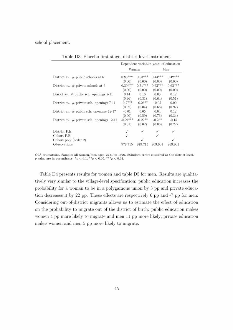
school placement.

Table D3: Placebo first stage, district-level instrumentDependent variable: years of education

Women Men

District av. # public schools at 6 0.85*** 0.83*** 0.44*** 0.42***(0.00) (0.00) (0.00) (0.00)

District av. # private schools at 6 0.30*** 0.31*** 0.63*** 0.63***(0.00) (0.00) (0.00) (0.00)

Disrict av. # public sch. openings 7-11 0.14 0.16 0.08 0.12(0.36) (0.31) (0.64) (0.51)

District av. # private sch. openings 7-11 -0.27** -0.26** -0.05 0.00(0.02) (0.04) (0.68) (0.97)

District av. # public sch. openings 12-17 -0.01 0.05 0.04 0.12(0.90) (0.59) (0.76) (0.34)

District av. # private sch. openings 12-17 -0.29*** -0.22** -0.25* -0.15(0.01) (0.02) (0.06) (0.22)

District F.E. X X X XCohort F.E. X XCohort poly (order 2) X XObservations 979,715 979,715 869,901 869,901

OLS estimations. Sample: all women/men aged 25-60 in 1976. Standard errors clustered at the district level.p-value are in parentheses. *p < 0.1, **p < 0.05, ***p < 0.01.

Table D4 presents results for women and table D5 for men. Results are qualita-tively very similar to the village-level specification: public education increases theprobability for a woman to be in a polygamous union by 3 pp and private educa-tion decreases it by 22 pp. These effects are respectively 6 pp and -7 pp for men.Considering out-of-district migrants allows us to estimate the effect of educationon the probability to migrate out of the district of birth: public education makeswomen 4 pp more likely to migrate and men 11 pp more likely; private educationmakes women and men 5 pp more likely to migrate.

45

Table D4: Results of 2SLS regressions, instrument at the district level, womenSample of all women Sample of married women

(1) (2) (3) (4) (5) (6) (7) (8) (9) (10) (11)Wage Agric. Ever Husband’s Husband Husband Husband Husband’s # Wife Husband’searner worker Migrant married education wage earner migrant polygamous of wives rank age

Instrument: district average # of public schools in the village at 6controlling for district and cohort fixed effects

Years of schooling 0.04*** -0.04*** 0.04*** -0.02*** 0.72*** 0.06*** 0.03*** 0.03** 0.10*** 0.00 0.20(0.00) (0.00) (0.00) (0.00) (0.00) (0.00) (0.00) (0.02) (0.00) (0.80) (0.48)

F-Stat of first stage 34.86 33.46 26.72 26.65 21.27 20.23 21.27 21.27 21.27 21.26 21.27

Instrument: district average # of private schools in the village at 6controlling for district and cohort fixed effects

Years of schooling 0.06*** -0.12*** 0.05** -0.12** 1.02*** 0.11*** 0.02 -0.22** -0.86** -0.28** -2.12(0.00) (0.01) (0.05) (0.02) (0.00) (0.00) (0.20) (0.01) (0.02) (0.04) (0.17)

F-Stat of first stage 3.24 2.72 6.13 6.16 6.62 7.37 6.61 6.63 6.63 6.61 6.61

Observations 513,164 511,456 979,715 976,474 691,229 634,367 692,285 689,820 689,820 692,295 692,267

Sample: all women aged 25-60 in 1976. Standard errors clustered at the district level. p-value are in parentheses. *p < 0.1, **p < 0.05, ***p < 0.01.

46

Table D5: Results of 2SLS regressions, instrument at the district level, menSample of all men Sample of married men

(1) (2) (3) (4) (5) (6) (7) (8)Wage Agric. Ever Wife(s)’s Number of Wife(s)’searner worker Migrant married education Polygamous Wives age

Instrument:district average # of public schools in the village at 6controlling for district and cohort fixed effects

Years of schooling 0.09*** -0.11*** 0.11*** 0.02 1.56*** 0.06 0.12 -1.91***(0.00) (0.00) (0.00) (0.41) (0.00) (0.11) (0.11) (0.00)

F-Stat of first stage 8.34 8.21 8.80 8.63 5.94 5.79 5.77 5.94

Instrument: district average # of private schools in the village at 6controlling for district and cohort fixed effects

Years of schooling 0.07*** -0.05*** 0.05*** -0.10*** 0.82*** -0.07*** -0.11*** 0.41(0.00) (0.00) (0.00) (0.00) (0.00) (0.00) (0.00) (0.26)

F-Stat of first stage 22.06 26.67 22.95 23.08 23.28 22.82 22.58 23.14

Observations 788,595 710,147 869,901 863,775 609,461 657,394 654,568 610,573

Sample: all men aged 25-60 in 1976. Standard errors clustered at the district level. p-value are in parentheses. *p < 0.1, **p < 0.05, ***p < 0.01.

47

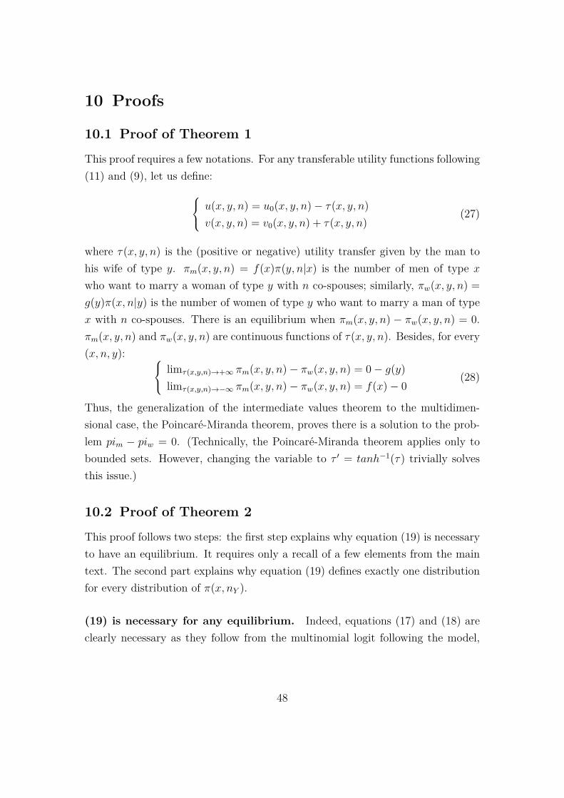
10 Proofs

10.1 Proof of Theorem 1

This proof requires a few notations. For any transferable utility functions following(11) and (9), let us define:

u(x, y, n) = u0(x, y, n)− τ(x, y, n)v(x, y, n) = v0(x, y, n) + τ(x, y, n)

(27)

where τ(x, y, n) is the (positive or negative) utility transfer given by the man tohis wife of type y. πm(x, y, n) = f(x)π(y, n|x) is the number of men of type xwho want to marry a woman of type y with n co-spouses; similarly, πw(x, y, n) =g(y)π(x, n|y) is the number of women of type y who want to marry a man of typex with n co-spouses. There is an equilibrium when πm(x, y, n) − πw(x, y, n) = 0.πm(x, y, n) and πw(x, y, n) are continuous functions of τ(x, y, n). Besides, for every(x, n, y): limτ(x,y,n)→+∞ πm(x, y, n)− πw(x, y, n) = 0− g(y)

limτ(x,y,n)→−∞ πm(x, y, n)− πw(x, y, n) = f(x)− 0(28)

Thus, the generalization of the intermediate values theorem to the multidimen-sional case, the Poincaré-Miranda theorem, proves there is a solution to the prob-lem pim − piw = 0. (Technically, the Poincaré-Miranda theorem applies only tobounded sets. However, changing the variable to τ ′ = tanh−1(τ) trivially solvesthis issue.)

10.2 Proof of Theorem 2

This proof follows two steps: the first step explains why equation (19) is necessaryto have an equilibrium. It requires only a recall of a few elements from the maintext. The second part explains why equation (19) defines exactly one distributionfor every distribution of π(x, nY ).

(19) is necessary for any equilibrium. Indeed, equations (17) and (18) areclearly necessary as they follow from the multinomial logit following the model,

48

and they imply (19).

There is a single distribution following (19) This step proves that, for everydistribution of the g(y) and f(x, nY ), there are several vectors a and b that definea distribution following (19); but each of these vectors define the same distributionπ(x, y, nY ).Firstly, let us introduce the notation Φ = exp φ

2 , and let a be the vector of allthe a(x, nY ), and b be the vector of all the b(y).It is possible to write the density g(y) as a function of a and b:

g(y) =∑x,n

Φ(x, y, n) exp((−a(x, n)− b(y))/2) (29)

By(a) := exp(−b(y)/2) = g(y)∑x,n Φ(x, y, n) exp(−a(x, n)/2) (30)

∂By(a)∂a(x, n) = By(a)πa(x, y, n)

2g(y) (31)

where πa(x, y, n) := Φ(x, y, n) exp(−a(x, n)/2)By(a) is the number of matches oftype x, n, y implied by a and the accountability of women in (29). Similarly,πa(x, n) = ∑

y πa(x, y, n) is the number of males of type x, n implied by a.We search for the vectors a ∈ IRk such that πa(x, n) = f(x, n) for every (x, n),

and we show that all the solutions lead to the same density.11

Firstly, there is always a vector a that solves πa(x, n) = f(x, n) for every (x, n).Indeed, πa(x, n) is a continuous function of a and for every (x, n):

lima(x,n)→+∞ πa(x, n) = 0lima(x,n)→−∞ πa(x, n) = ∑

y g(y) = 1(32)

Thus, the generalization of the intermediate values theorem to the multidimen-sional case, the Poincaré-Miranda theorem, proves there is a solution to the prob-lem. (Technically, the Poincaré-Miranda theorem applies only to bounded sets.However, changing the variable to a′ = tanh−1(a) trivially solves this issue.)

11k is the number of points on the support of x, n

49

Secondly, let us study the gradient of πa(x, n). The partial derivatives of πa are:

∂πa(x, n)∂a(x, n) = 1

2∑y

(−1 + πa(x, y, n)

g(y)

)πa(x, y, n) (33)

when x′ 6= x or y′ 6= y:

∂πa(x, n)∂a(x′, n′) = 1

2∑y

πa(x′, y, n′)g(y) πa(x, y, n) (34)

Let u = (u(x, n)) be a vector that defines a direction in the space of the vector a.Then:

gradπa(x, n) · u = −12∑y

πa(x, y, n)u(x, n)−

∑x′,n′

u(x′, n′)πa(x′, y, n′)g(y)

(35)

Here, ∑x′,n′ u(x′, n′)πa(x′,y,n′)g(y) is the weighted average of the u(x′, n′), where the

weights follow the distribution of the x′, n′ conditionnal on y implied by a. Hence,for xm, nm such that u(xm, nm) is maximal, the sign of (35) is constant. Two casesemerge:

• For every x, n, u(x, n) = α ∈ IR. gradfx,n(a) · u = 0: the densities areunchanged for a variation of a in this direction. The reason is the following:if a(x, n) increase by α for every x, n and b(y) decrease by α for every y,equation (19) is unchanged.

• u(x, n) depends on x, n, u(xm, nm) > u(x, n) for some x, n, and gradfxm,nm(a)·u < 0. For any line of the space following the direction defined by u, there isexactly one point such that fxm,nm(a) = π(xm, nm). So there is at most onepoint such that fx,n(a) = π(x, n) for every (x, n).

So for every line of the space, there is at most single density following equation(19), g(y) and f(x, n). There cannot be several densities over IRk (IRk is a stardomain).

50