Manuscript prepared for Atmos. Chem. Phys. Discuss.with version 2.2 of the LATEX class copernicus discussions.cls.Date: 13 June 2014

Transport of aerosol to the Arctic: analysis ofCALIOP and French aircraft data during thespring 2008 POLARCAT campaignG. Ancellet1, J. Pelon1, Y. Blanchard1, B. Quennehen2,1, A. Bazureau1, K.S. Law1,and A. Schwarzenboeck2

1Sorbonne Universite, UPMC, Paris 06; Universite Versailles St-Quentin; CNRS/INSU;LATMOS2Universite B. Pascal; INSU/CNRS; Laboratoire de Meteorologie Physique

Correspondence to: G. Ancellet (gerard.ancellet@upmc.fr)

1

Abstract

Lidar and in situ observations performed during POLARCAT campaign are reported here interms of statistics to characterize aerosol properties over northern Europe using daily airbornemeasurements conducted between Svalbard Island and Scandinavia from 30 March to 11 April2008. It is shown that during this period, a rather large number of aerosol layers was observedin the troposphere, with a backscatter ratio at 532 nm of 1.2 (1.5 below 2 km, 1.2 between 5 and7 km and a minimum in-between). Their sources were identified using multispectral backscat-ter and depolarization airborne lidar measurements after careful calibration analysis. Transportanalysis and comparisons between in situ and airborne lidar observations are also provided toassess the quality of this identification. Comparison with level 1 backscatter observations of thespaceborne CALIOP lidar were done to adjust CALIOP multispectral observations to airborneobservations on a statistical basis. Re-calibration for CALIOP daytime 1064 nm signals led to adecrease of their values by about 30% possibly related to the use of the Version 3.0 calibrationprocedure. No re-calibration is made at 532 nm eventhough 532 nm scattering ratios appear tobe biased low (-8%) because there are also significant differences in air mass sampling betweenairborne and CALIOP observations. Re-calibration of the 1064 nm signal or correction of -5%negative bias in the 532 nm signal both could improve the CALIOP aerosol color ratio expectedfor this campaign. The first hypothesis was retained in this work. Regional analyses in theEuropean Arctic then performed as a test, emphasize the potential of the CALIOP spacebornelidar to further monitor more in depth properties of the aerosol layers over Arctic using infraredand depolarization observations. The CALIOP April 2008 global distribution of the aerosolbackscatter reveal two regions with large backscatter below 2 km: the Northern Atlantic be-tween Greenland and Norway, and Northern Siberia. The aerosol color ratio increase betweenthe sources regions and the observations at latitudes above 70oN is consistent with a growth ofthe aerosol size once transported to the Arctic. The distribution of the aerosol optical propertiesin the mid troposphere supports the known main transport pathways between mid-latitudes andthe Arctic.

2

1 Introduction

It is recognized that long range transport of anthropogenic and biomass burning emissions fromlower latitudes is the primary source of aerosol in the Arctic (Quinn et al., 2008; Warneke et al.,2010). Frequent haze and cloud layers in the winter-spring period contribute to surface heatingby their infrared emission (Garrett and Zhao, 2006). The relative influence of the different mid-latitude aerosol sources was initially discussed by Rahn (1981) who concluded that the Eurasiantransport pathway is important using meteorological considerations and observations. Law andStohl (2007) also stressed the seasonal change of air pollution transport into the Arctic with afaster winter circulation implying a stronger influence of the southerly sources in the middleand upper troposphere.

During the International Polar Year in 2008, these questions were addressed in the frameof the Polar Study using Aircraft, Remote Sensing, Surface Measurements and Models, Cli-mate, Chemistry, Aerosols and Transport (POLARCAT) and Arctic Research of the Compo-sition of the Troposphere from Aircraft and Satellites (ARCTAS) field experiments. Aircraftobservations were conducted respectively in spring 2008 over the European Arctic as part ofPOLARCAT-France (Adam de Villiers et al., 2010; Quennehen et al., 2012) and over the NorthAmerican Arctic as part of ARCTAS (Jacob et al., 2010). Several papers have already been pub-lished on the characterization of aerosols over the western Arctic (Brock et al., 2011; Rogerset al., 2011; Shinozuka et al., 2011). Overall they provide a very useful data base to discuss theaerosol transport pathways and the main processes driving their evolution when transported tothe Arctic. Besides field experiments involving aircraft measurements, no systematic informa-tion was provided until recently on regional Arctic aerosols by space observations. The Cloud-Aerosol Lidar and Infrared Pathfinder Satellite Observation (CALIPSO) mission (Winker et al.,2009) has proven to be very useful to address these questions as illustrated by the recent workof Winker et al. (2013) although all its potential has not been explored yet. Recent studies usingthe Cloud-Aerosol Lidar with Orthogonal Polarization (CALIOP) level 2 products, namely the5 km aerosol layer products (AL2) at 532 nm gridded for the Arctic domain allowed aerosolextinction and aerosol optical depth (AOD) to be derived (Di Pierro et al., 2013). The main

3

features of transport in the Arctic were inferred from the seasonal variability of the verticaldistribution of aerosol, derived from AL2 version 3 products by Devasthale et al. (2011). Ob-servations by the CALIOP lidar provide the optical properties of aerosol layers at two differentwavelengths (532 nm, 1064 nm), but the infrared (IR) data have not been widely used due in alarge part to difficulties in the calibration of the level 1 (L1) products (Wu et al., 2011; Vaughanet al., 2012)). In our study we thus address this topic looking for the usefulness of the additionalinformation provided by the 1064 nm channel and depolarization measurements.

In this work, we focus on the European Arctic sector in spring 2008 using the data of thePOLARCAT-France experiment. The purpose of this paper is thus to discuss how CALIOPspaceborne lidar data can be compared to and combined with aircraft data in the western Arc-tic area to provide (i) a comparison of CALIOP observations with those from airborne lidar atsimilar wavelengths in a region where CALIOP data are very useful but not very well charac-terized (ii) tracks for bias correction and use of L1 CALIOP observations at 1064 nm and in thedepolarization channel to analyze behavior of color and depolarization ratios, respectively. (iii)an improved description of the spatial variability of aerosol sources and transport to the Arctic,and implications for a regional and monthly mean characterization.

We start in section 2 by a description of the aircraft campaign lidar data and the meteorologi-cal context which includes also a characterization of the particles from in situ measurements andair mass transport using the FLEXPART model. The POLARCAT France campaign was onlydescribed for some specific flights in previous papers (Adam de Villiers et al., 2010; Quennehenet al., 2012). In section 3.3, comparison between airborne and spaceborne data are addressed,looking to the statistical distribution and the spatial variability derived from all the aircraftflights available during POLARCAT-France, and coordinated CALIOP observations. In section4, results obtained with monthly averaged L1 CALIOP data in April 2008 are used to analyze(i) the link between the meridional variability of the aerosol properties in relation with the airmass origin (ii) the large scale horizontal variability in these aerosol properties in the wholeArctic domain. The latter is finally discussed with respect to the results obtained by previousanalysis involving CALIOP AL2 products.

4

2 The POLARCAT spring campaign

2.1 Campaign context and description

The French ATR-42 was equipped with remote sensing instruments (lidar, radar), in-situ mea-suring probes of gases (O3, CO) and aerosols (concentration, size distribution). The ATR-42deployment was often designed to collect data near to CALIOP satellite observations duringdaytime overpasses. The positions of the 12 scientific flights performed from 30 March to 11April 2008 (Fig.1) show that they are well suited for an analysis of the meridional distributionnear 20oE. The meteorological context in the Arctic in April 2008 is discussed in Fuelberg et al.(2010). The maps of the 700 hPa equivalent potential temperature (θe) and winds are howevershown in figure 1 and 2 of the supplementary information document to identify the variability ofthe position of the Arctic front. This front was near 71oN until 2 April and moved to lower lati-tudes near 68oN after 2 April. It is seen that flights were frequently performed in the air massesstrongly influenced by the southerly flow from Europe at the beginning of the campaign, whilelarge section of the flights were representative of the Arctic pristine air at the end of the cam-paign. After 9 April, the European Arctic at latitude above 70oN becomes strongly influencedby advection of biomass burning plumes advected from Asia (Quennehen et al., 2012).

The vertical structure of the aircraft flight plans were always chosen to have several in-situand airborne lidar measurements in similar air masses in order to study the representativenessof lidar products such as the attenuated backscatter, the color ratio and the depolarization ratio.

During the aircraft campaign, the CALIOP spaceborne instrument provided 80 satellite over-passes for the period 27 March to 11 April in the area: 65oN-80oN, 5oE-35oE (Fig.1). For thearea south of 72.5oN which corresponds to the aircraft deployment, there are 45 CALIOP tracksleading to 433 vertical profiles with 80 km horizontal resolution. In this work different temporalor spatial averaging will be used to analyze the CALIOP data either in the aircraft domain forcomparison with the airborne data (section 3.3) or in the whole European Arctic area for all thedays in April 2008 (section 4).

5

2.2 Aircraft data

2.2.1 Airborne Lidar measurements

During the POLARCAT campaign, the airborne lidar LEANDRE Nouvelle Generation, pro-vided measurements in its backscatter configuration (hereafter simplified as B-LNG) of totalattenuated backscatter vertical profiles at three wavelengths: 355, 532 and 1064 nm. An addi-tional channel recorded the perpendicular attenuated backscatter vertical profile at 355 nm. TheB-LNG lidar is already described in Adam de Villiers et al. (2010) (ADV2010) where a singleflight on 11 April 2008 was analyzed. The methodology to calibrate the attenuated backscatteris also fully described in ADV2010 so it is only briefly recalled here.

In this paper, aerosol layers are identified for the 12 flights using 20-s averages of lidar pro-files (i.e. a 1.5 to 2 km horizontal resolution). Only downward pointing lidar observations havebeen included in this work. The B-LNG data are first corrected for energy variations. Calibra-tion factors are then determined for each wavelength and for each flight by searching for areaswith very low aerosol content and by assuming that the Rayleigh contribution controls the lidarsignal. These areas are chosen, as far as possible, in the upper altitude range close to the aircraftwhere bias due to the aerosol transmission does not play a significant role. The consistency ofthe calibration factor is checked using different aerosol free areas, and several flights, when-ever possible. This is the major source of error in the calculation of R(z), and the uncertainty(error + bias, but mostly due to bias) was found to be less than 15% at 532 nm and less than30% at 1064 nm. These numbers were derived from a sensitivity study using different possiblecalibration factors and different flights. The two 355 nm channels are calibrated independentlyusing molecular reference and the ratio of the total perpendicular- to the total parallel-polarizedsignals. However, due to a reduced field of view at 355nm, the overlap of the emitted beam withthe receiver field of view limits our ability to calibrate independently the total 355 nm lidar sig-nal in the areas near the aircraft selected at the other wavelengths. Therefore, and as CALIOPis operating at 532 nm, the measurements at 355 nm are only used for the depolarization ratioanalysis, which is less dependent on the geometrical factor. The B-LNG 355 nm ratio is onlya proxy for the CALIOP one, as some differences are expected to occur due to wavelength

6

difference (Freudenthaler et al., 2009).The aerosol parameters discussed in this paper and the way to calculate them, are fully de-

scribed in ADV2010. They are the same for airborne and spaceborne observations (althoughdepending on the wavelength for depolarization). They are namely (i) the attenuated backscatterratios R(z) at 532 nm and 1064 nm using the CALIOP atmospheric density model to cal-culate the Rayleigh backscatter vertical profiles, (ii) the ratio of the total perpendicular- tothe total parallel plus perpendicular polarized backscatter coefficient (or pseudo depolariza-tion ratio (PDR) δ355) at the measurement wavelength, 355 or 532 nm, respectively, (iii) thepseudo color ratio defined as the ratio of the total backscatter coefficients at 1064 and 532 nm(PCR(z)=R1064(z)/[16R532(z)] (iv) the color ratio defined as the ratio of the aerosol backscat-ter coefficients at 1064 and 532 nm (CRa(z)=(R1064(z)−1)/[16(R532(z)−1)]). The aerosolcolor ratio can be also written as CRa(z) = 2−k, where k is an exponent depending on theaerosol microphysical properties (Cattrall et al., 2005).

The vertical and latitudinal aircraft cross sections are listed in Table 1 and the correspondingR532 sections are shown in Fig.3 of the supplementary information document. Clouds areremoved from the lidar signals using a threshold both in scattering ratio and depolarization.

This dataset composed of 18 lidar meridional cross sections is a representative sample of theEuropean Arctic spring aerosol distribution, as it includes different kinds of aerosol load in thelower troposphere and several cases of aerosol layers detected in the troposphere above 2 km.The probability density function (PDF) of the retrieved R(z) are shown in Fig.2 to check thatthe lidar data processing does not produce outliers for some flights. The homogeneity of theresults between the different flights has also been verified by dividing the lidar data into threesubsets: one corresponding to the beginning of the campaign (before 7 April) , the second oneto the end (after April 7), and the third to the overall campaign (see Table 1 ) . The differencesbetween the 3 subsets are small when looking at the means and standard deviations of thedistributions meaning that the error related to the calibration procedure is independent of theselected flight (not shown). In Fig.2, the R532(z) values do not exceed 2 (90th percentile=1.45)with a mean value of 1.2, as expected for the Arctic troposphere where there are a lot of airmasses with a low aerosol load (Rodrıguez et al., 2012). Both the IR and the green distribution

7

show a high left tail in the histogram. Although most of the aerosol scattering ratios are foundnear the median values (R532=1.15 and R1064=1.9), the high left tail show that air masses withR532>1.4 and R1064>2.8 are also frequently found (probability > 75%). The uncertainty ofthe mean values R532 and R1064 can be evaluated assuming 100 independent samples for the18 cross sections shown in Fig.3 of the supplementary document, (i.e. 3 vertical layers and 2horizontal layers) and errors of 0.1 and 0.5 for R532 and R1064, respectively, in a single layer.The distribution of the aerosol color ratio shows a mean CRa near 0.31±0.12, correspondingto a rather large wavelength dependence, and thus to small particle size (k=2). A small mode isseen to occur near 0.5 corresponding to much smaller wavelength dependence (k=1) and thusto larger particles. We also obtain a value of 0.33± 0.04 for the color ratio CRa

∗= R1064−1

16(R532−1)

calculated using the mean values of R(z) (Fig.2). Larger values near 0.5 are explained by thefact that at least 20% of the 532 nm observations with moderate R532 values near 1.2 contributeto the tail of the R1064 distribution with values than 2.4. The CRa values from the B-LNG aresmaller than the range 0.4-1 (dust excepted) derived from the AERONET network using sunphotometers at 26 sites across the globe (Cattrall et al., 2005). However similar values havebeen reported for polar air masses using lidar measurements in Alaska and Canada (Burtonet al., 2012) and for a smoke layer over Ny-Alesund (Stock et al., 2011).

Since in Fig. 2, the backscatter ratio distributions points toward a significant contribution ofaerosol particles with small sizes, we thus looked at in situ measurements where comparisonsare possible.

2.2.2 Comparison of airborne lidar with in-situ measurements

Aerosol and carbon monoxide (CO) in-situ measurements available on the ATR-42 aircraftare described in Quennehen et al. (2012) and ADV2010. For the aerosols, a condensationparticle counter (CPC-3010) measured the number of submicronic particles, while the aerosolconcentrations in different size bins were measured by a Passive Cavity Aerosol SpectrometerProbe (PCASP SPP-200), a GRIMM (model 1.108), and a Scanning Mobility Particle Sizer(SMPS) with a lower time resolution (150 s). In this paper we have used the SMPS and the

8

Grimm data to compute the aerosol mean geometrical diameter with the 150 s time resolution.Comparisons of the CPC concentrations with the integrated concentrations of the 8 size bins ofthe GRIMM between 0.3 and 3 µm, provide estimates of the relative fractions of coarse sizeaerosol.

For flights with frequent vertical motion of the aircraft, it is easy to verify the comparabilityof lidar and in-situ data. Such a comparison involves looking at in-situ measurements onlyduring aircraft ascents or descents crossing aerosol layers that the lidar detects later or earlier,respectively. An example of a comparison of the lidar attenuated backscatter measured 150m below the aircraft with CO and the CPC concentrations is shown in Fig.3 for the last flighton 11 April 2008, where rather large aerosol scattering ratios were measured (see Fig.3 ofthe supplementary information document). No delay correction is performed in this figure tocompensate for aircraft speed and lidar measurement distance (this is not detectable at thisscale), but a high correlation (0.55 with a significance better than 99%) is nevertheless observedbetween lidar backscatter ratio and aerosol particle concentration.

Ten independent aerosol layers seen at nearly the same time by the lidar and the other in-struments on-board can be used for a meaningful comparison of the lidar parameters (color anddepolarization ratios) with the aerosol concentration and size spectrum (Table 2). The CO mix-ing ratios are well correlated with the CPC data implying that combustion aerosols were oftenencountered with the largest concentrations at the end of the campaign. Changes in the pseudocolor ratio PCR measured by the airborne lidar correspond quite well to the variations in theaerosol mean diameter because R532 variations are small enough for these 10 layers to insure aweak dependency with the aerosol concentration (Fig. 3). The increase ofCRa from 0.2 to 0.35is also in good agreement with the variation in the aerosol mean geometrical diameter if we ex-clude the cases with the largest error on CRa. The uncertainty in the color ratios are calculatedassuming a 30% and 15% relative uncertainty for the IR and green scattering ratio respectively.According to Table 2, the largest color ratios also correspond to the largest integrated GRIMMconcentrations which are high for layers with coarse size aerosol. The PCR and CRa valuescalculated by the airborne lidar can be then considered as valuable proxies for evaluating thecontribution of the coarse aerosol fraction, and to first order (not considering speciation and

9

size) the lidar backscatter ratio is a good indicator of aerosol content.

2.3 Characterization of air mass transport

The origin of the air masses sampled during the aircraft campaign by the B-LNG lidar and byCALIOP was studied using the FLEXPART model version 8.23 (Stohl et al., 2002) driven by6-hourly ECMWF analyses (T213L91) interleaved with operational forecasts every 3 hours. Ata given location the model was run to perform domain filling calculations in 13 boxes from 1- to7.5-km altitude with a horizontal dimension of 1ox 1o. The transport from the different regionsare considered for two altitude ranges: < 3 km and between 3 and 7 km in order to distinguishthe two major transport pathways to the Arctic: low level flow over cold surfaces, upper leveladvection by an uplifting along the tilted isentropes (Fuelberg et al., 2010; Stohl et al., 2006).This was done along the 18 aircraft cross sections and the 80 CALIPSO tracks in the EuropeanArctic domain shown in Fig.1. For each box, 2000 particles were released during 60 minutesand the dispersion computed for 6 days backward in time. Longer simulations lead to largeruncertainties in the source attribution and are not considered in this work. We have introducedin the FLEXPART model the calculation of the fraction of particles originating below the 3 kmaltitude level for 3 areas with continental emissions shown in Fig.4 (Europe, Eurasia, NorthAmerica). We have also calculated the fraction of particles present at latitudes above 70oN inthe troposphere above the eastern Arctic and western Arctic (black boxes in Fig.4). The use ofthe eastern Arctic fraction is necessary to identify the role of the Eurasian sources because withour limited simulation time (6 days), we underestimate the role of aged air masses related toEurasian emissions (ADV2010).

The results first show negligible influence of the transport from the lower troposphere aboveNorth America and are not considered further here. The fraction of air mass origins for theother regions is shown for different latitude bins in Fig. 5. The meridional distribution andthe relative influence of the different regions are rather similar for the CALIPSO tracks and theairborne lidar flights in the lower atmosphere. However in the mid-troposphere, the increaseof the relative influence of the Eastern Arctic air versus European air masses is clearly shiftedtowards higher latitudes (74oN) for CALIOP (no contribution in the 71 oN -72oN latitude band

10

as seen for the airborne data). For both data set, the transport of air masses from the EasternArctic show a clear latitudinal increase in the lower altitude range just north of the polar front.For latitudes above 73oN, seen only by CALIOP, the overall influence of all the selected sourceregions on a time scale shorter than 6 days remains however smaller than 40% implying thata large fraction of air masses had stayed for more than 6 days in the European Arctic sectorlocated between -15oW and 30oE. Dilution, mixing and decay of the aged mid-latitude sourcesare to be expected at these latitudes. The main differences between CALIOP and the airbornelidar sampling are (i) a significant contribution from Eurasian sources at low latitudes for theaircraft data (ii) a weaker contribution of the Eastern Arctic sector in the mid-troposphere forCALIOP, especially around 70-72 oN. For the airborne lidar, the Eurasian sources are not onlytransported into the Arctic above the Pacific western coast but also by a low level southerly flowover eastern Europe from 6 to 9 April 2008. These differences are most probably due to themuch larger longitude band selected for the analysis of the CALIOP data set (5oW to 35oW)Despite these differences, the overall similarity of the transport regime for both data sets is agood indication that the small number of aircraft flights is fairly representative of the influenceof the different source regions, and the data gathered may be used to compare retrieved aerosolproperties in the campaign area.

3 Analysis of CALIOP data during the aircraft campaign

3.1 Methodology of the CALIOP data processing

A detailed description of the CALIOP operational processing can be found in a series of papers(Vaughan et al., 2009; Liu et al., 2009; Omar et al., 2009; Powell et al., 2009). Uncertainties inthe AL2 color ratio and the depolarization ratio are often very large and they are mainly usedfor a qualitative analysis of the aerosol composition and evolution (see Omar et al. (2009) forinterpretation of the color ratio and the depolarization ratio for aerosol classification). Most ofthe error in the color ratio finds its origin in the signal calibration. More recently, analyses havebeen conducted to improve the calibration in version 4 (Vaughan et al., 2012), that confirmed a

11

bias in the 1064 nm channel and to a small extent the one in the 532 nm daytime channel. Wethus considered a comparison between airborne and spaceborne CALIOP L1 observations as afirst step.

In ADV2010, the AL2 CALIOP products were analyzed for one particular flight of the PO-LARCAT campaign using layers detected at 80-km horizontal resolution and with a 3% thresh-old value for the layer optical depth at 532 nm. Comparisons between the CALIOP AL2 andairborne lidar PCR then showed larger values for CALIOP in the aerosol layers of the 11 Aprilflight. Considering the large uncertainty in the weak aerosol layers detected in the AL2 productover the Arctic, averaging of the L1 version 3.01 CALIOP data are used in this paper to ana-lyze the 45 CALIPSO tracks available in the aircraft campaign domain. The comparison of theaerosol parameter PDF obtained for the campaign period and the campaign area is considered asmore appropriate to validate the satellite aerosol data than relying on optimized collocations ofaircraft and satellite data, which would give a very small number of cases. Gridded latitudinaldistributions with a 1.5o resolution in the campaign area are used to check the coherency of thetwo data sets.

The CALIOP L1 attenuated backscatter coefficients β1064 and β532, are available with an333 m horizontal resolution up to the 8.2 km vertical level and it is 1 km at higher altitude.Before making any horizontal or vertical averaging of these data, it is necessary to apply acloud mask on the L1 data set. This cloud mask is based on the cloud mask features available inthe level 2 version 3.01 CALIOP cloud (CL2) data products for the 5-km horizontal resolution.Additional checks have however been added to verify that cloud layers are not misclassified.First, ice cloud layers, detected in the 80 km horizontal resolution profile, must have a pseudocolor ratio > 0.6 and a layer depolarization ratio > 0.3. If this is not the case, the 3 brightnesstemperatures T12µm, T10µm, T8µm measured by the IR Imaging Radiometer (IIR) installed onthe same platform (Garnier et al., 2012), are used as an additional test to keep the layer as acloud layer or not. Based on simulations, the criteria to keep a layer as a cloud layer is that thedifferences T8µm-T12µm and T10µm-T12µm must be positive (Dubuisson et al., 2008). Second,if the cloud layer is also detected in the 333-m resolution CL2 data products, it is always keptas a cloud as explained in Liu et al. (2009). Only very dense aerosol layers (scattering ratio >

12

3) are misclassified when adding these two conditions.The β1064 and β532 data are then removed below the highest cloud top altitude for each ver-

tical profile, when the optical depth (OD) of the cloud is larger than 1. For semi-transparentclouds with smaller ODs (<0.9), a transmission correction is performed. The data are also ex-cluded in the 100 m layer just above the cloud top to avoid any error in the cloud top estimate.The cloud filtering is then very conservative in order to exclude a possible bias in the aerosol pa-rameters measured below clouds when the spectral variation of the overlaying cloud attenuationhas to be taken into account.

The cloud filtered 333-m attenuated backscatter vertical profiles are then averaged horizon-tally over 80 km and vertically over 150 m with a low pass 2nd order polynomial filter toimprove the signal to noise ratio. The 80-km mean attenuated backscatter ratio R532(z) andR1064(z), the mean aerosol color ratio, and the mean 532-nm volume depolarization ratio arefinally calculated using the molecular density and ozone vertical profiles available at 33 standardaltitudes in the CALIOP data products.

As explained before two different methods are used for the comparison with airborne lidarobservations:

– PDF of aerosol parameters using all the 80 km, 150 m averaged profiles available in theaircraft campaign area, i.e. with 0<z<7 km, 65oN<latitude<72.5oN, 5oE < longitude <35oE, from 27 March to 11 April 2008

– latitudinal cross section in the same campaign area where 80 km, 150 m averaged profilesare gridded into 5x14 boxes with a 1.5olatitude and 500 m vertical resolution.

3.2 Impact of the 1064 nm CALIOP calibration on the aerosol color ratio

TwoR532(z) mean profiles out of the 1.5ogridded data set are compared with the correspondingR1064(z) mean profiles in Fig.6. TheR1064(z) is scaled toR532(z) to facilitate the comparison,assuming two extreme values of the expected aerosol color ratio CRa (0.5 and 1), the range ofvalues proposed by Cattrall et al. (2005). This corresponds to factors of 8 and 16, respectivelyin the scaling of R1064(z)-1. For both latitude bins, a good consistency is obtained between

13

the aerosol vertical structures at both wavelengths showing that the proposed averaging reducesthe noise at a level high enough to detect the mean aerosol layering at 1064 nm. The layer at8 km can be used to identify the appropriate aerosol color ratio because the spectral variationof the aerosol attenuation of the signal above the layer is not very important. With the lidar1064 nm calibration factor used in the Version 3 CALIOP L1 data products (see top figuresin Fig.6), the ratio between R532(z)-1 and R1064(z)-1 in this upper layer leads to CRa near 1for both examples. This would mean that large dust like aerosols contribute in both cases tothe tropospheric aerosol in the European Arctic sector no matter which latitude band is chosen,which does not seem to be credible. Furthermore depolarization remains low (< 5%).

The 1064 calibration in the Version 3 CALIOP data set is based on the assumption that fora specific set of cirrus cloud the cloud color ratio is equal to 1 which allows to transfer the 532nm calibration to the 1064 channel. This is detailed in a large number of publications (Vaughanet al., 2010, 2012; Reagan et al., 2002; Winker et al., 2013) The cirrus cloud selection in Version3 implies an altitude range between 8 and 17 km and a minimum scattering ratio (>50). Thenumber of cirrus cloud with these characteristics are too small (<11) for the campaign domainand period and no additionnal check was done to verify the cirrus color ratio.

To reconcile the aerosol color ratio with the expected value, 3 options are possible to decreasethe 1064 total backscatter, to increase the 532 nm total backscatter, or change both parameters.Considering first the uncertainty of the 1064 nm channel (Vaughan et al., 2012) and second thedifficulty to estimate the respective impact of sampling differences and calibration error of the532 nm CALIOP data (see section 3.3), the 532 nm total backscatter value were not adjusted tothe airborne data. The choice was to apply instead an a priori fixed multiplicative factor on the1064 nm total backscatter, assuming a 40% and 30% overestimate for daytime and nighttimeconditions, respectively. For daytime this is estimated from the B-LNG mean scattering ratios(see Fig.2). A reduced value was considered for nighttime, as linked to the ratio in the daytimeand nighttime scale factors in Version 3 CALIOP data as mentioned in previous analysis (Wuet al., 2011; Vaughan et al., 2012). The ratio between R532(z)-1 and R1064(z)-1 then becomesmore realistic since it leads to CRa intermediate between 0.5 and 1 for the upper layer near 8km, but also for the layers in the lower troposphere.

14

To verify that large CRa for uncorrected IR data is not related to a bias introduced by theaveraging of many profiles before the calculation of the color ratio, we have looked at theR532(z) versus R1064(z) scatter plot using all the 80 km resolution CALIOP filtered data forthe altitude ranges, 0-7 km and 13-15 km. The scatter plots are presented in Fig. 7 for theuncorrected and corrected IR data using a frequency contour plot. Since we expect a very weakaerosol contribution in the 13-15 km altitude range, no specific correlation are found betweenR532(z) versus R1064(z). The noise of the 532-nm attenuated backscatter is of the order of0.15 x molecular backscatter while the noise of the 1064-nm attenuated backscatter is 3 and 4x molecular backscatter with and without the correction of IR data, respectively. Accountingfor the factor 16 between the two molecular contributions, the noise in the IR channel is only1.2 larger than the 532-nm noise value when correcting the IR data. Such a ratio is comparableto the analysis of Wu et al. (2011) at 16 km for all the daytime CALIOP data. No correctionof the IR would mean a ratio of 1.7 between the 532-nm and 1064-nm signal noise level. Theoverestimate of the 1064-nm backscatter is even more likely when looking at the scatter plot forthe altitude range 0-7 km. The slope of the regression line is indeed too small for the uncorrectedIR data since it corresponds to many CRa values larger than 1. The frequency of clean airmasses (R=1) is also more consistent between the 532-nm and the 1064-nm observations afterthe correction of the IR overestimation provided that the 532 nm scattering ratio is correct.

The impact on the cirrus color ratio was not evaluated for the small number of occurencesin our domain but it would imply a positive bias of 40% when using the Version 3 calibration.Such a bias is larger that the uncertainty of ± 20-30% proposed for the 1064 nm calibrationprocedure (Wu et al., 2011; Vaughan et al., 2012). We must recall however that a 40% bias canbe also accounted for if we assume a negative bias of 5% for the 532 nm scattering ratio. Asexplained in section 3.3, this hypothesis was not considered in this work and the re-calibrationof the 1064 nm signal was chosen. It will be interesting to test this hypothesis using the newVersion 4 level 1 Caliop data which becomes now available. In the new version 4, the cirruscloud selection for the 1064 calibration (i.e. with a cloud color ratio of 1) is now different (cloudtemperature instead of altitude selection, use of the cloud depolarization ratio) providing morecirrus clouds and better altitude selection for the Arctic (Vaughan et al., 2012). .

15

3.3 Comparison of airborne lidar and CALIOP

3.3.1 Analysis of the statistical distribution

Using the dataset averaged over the campaign period/domain, the distributions of the CALIOPcorrected R1064 and R532 are shown in Fig. 8 for the range 0-7 km and 13-15 km. The lattercorresponds to very low aerosol concentrations. It has a mean and a median with a differenceless than 0.02 at 532 nm and 0.3 at 1064 nm from the expected scattering ratio of 1. The largestandard deviations of 0.3 at 532 nm and 4 at 1064 nm is expected at this altitude level wherethe molecular backscatter decreases significantly.

The R1064 mean (2.3) is close to the airborne lidar value (2.1) considering an error of themean of the order of 0.1 and even though the standard deviation of the noisy CALIOP R1064

distribution is 1.7 times larger than the airborne lidar corresponding value. The same ratio isobserved between the airborne and CALIOP R532 standard deviation. Therefore, this confirmsthe validity of the estimated correction factor, although with a large statistical error (about 30%on the coefficients) for the 1064 nm CALIOP profiles selected in our study of the Arctic region.

Contrary to the airborne lidar distribution, the CALIOP R532 distribution in the tropospherebelow 7 km does not show many layers with elevated aerosol concentrations as shown by alower value of the 90th percentile (1.34 for CALIOP instead of 1.45 for the airborne lidar).The larger standard deviation (0.34 instead of 0.2) is related to the poorer signal to noise ratioof the satellite dataset. The lower value for the 532 nm mean (1.13 instead of 1.21) is largerthan the expected uncertainty on the mean of the CALIOP distribution which is of the order of0.01. This uncertainty of the mean is calculated assuming an error of 0.4 for a single CALIOPmeasurement (i.e. the width of the distribution for the negative values) and assuming 1700independent layers out of 28872 data points available in the 0 and 7 km altitude range abovethe campaign domain (i.e. considering a 1 km vertical sampling instead of the 60 m verticalresolution to ensure independence). Since we compare patchy data, it is also important to assesshow the averaging of aerosol layers with observed clear air scenes may explain this difference.For example the difference between the airborne and CALIOP R532 means can be explained ifthere are twice as many layers with low aerosol load (R532< 1.05) in the CALIOP data set. This

16

may be related to the fact that we remove in our CALIOP data processing all the total backscattervalues below clouds. We must also check whether this difference may also be due to (1) anoverestimate of the 532 nm CALIOP calibration factor (2) an underestimate of the airborne lidarcalibration factor. Positive differences due to 532 nm daytime calibration uncertainty were alsoobtained by (Rogers et al., 2011) when comparing NASA HSRL airborne lidar and CALIOPdata for measurements at high latitudes in the Northern Hemisphere, but the mean difference isnot higher than 3%. The remaining 5% uncertainty on the mean difference can be accountedby a systematic error in the airborne lidar calibration when assuming no aerosol in the altituderange which corresponds to the smallest attenuated backscatter coefficient. Comparisons withother observations confirmed that 532 nm CALIOP data could be underestimated by about 5%,due to the occurrence of residual stratospheric aerosols at the normalization altitude (Vernieret al., 2009). This would be supported by the fact that we obtain a very small value (<2%) ofthe 532 nm mean aerosol scattering ratio in the 13-15 km range when using the Version 3.0calibration.

The averageCRa is 0.44±0.8 for CALIOP which is not very far from the airborne lidar value(0.31±0.12) considering the factor of 6 between the two standard deviations of this parameter(Fig. 8). For the noisy satellite data, a better proxy is CRa

∗=0.65±0.1, i.e. the mean color ratiocalculated with (R532-1) and (R1064-1), which is then 2 times larger than the similar ratio forthe airborne lidar. This can be explained by the 10% bias in R532 which are always less than1.35. Therefore this difference cannot be interpreted as a stronger contribution of the coarsesize aerosol fraction in the satellite observations. Despite this bias in the order of magnitude ofCRa

∗, it is important to verify if the relative spatial or temporal variability is detected by thesatellite data.

3.3.2 Analysis of the latitudinal distribution

The latitudinal variability of the aerosol properties is studied using the CALIOP latitudinal griddata set described earlier, i.e. considering 5 successive 1.5 olatitude bins and 14 vertical layersof 500 m. The airborne lidar data are analyzed only for layers where the aerosol content ishigh enough to be observed in the 1064 nm profiles. There are 90 well defined and independent

17

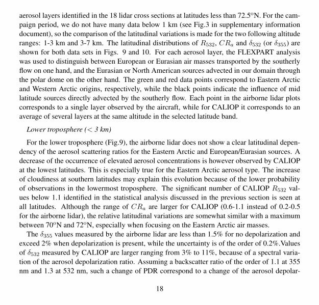
aerosol layers identified in the 18 lidar cross sections at latitudes less than 72.5oN. For the cam-paign period, we do not have many data below 1 km (see Fig.3 in supplementary informationdocument), so the comparison of the latitudinal variations is made for the two following altituderanges: 1-3 km and 3-7 km. The latitudinal distributions of R532, CRa and δ532 (or δ355) areshown for both data sets in Figs. 9 and 10. For each aerosol layer, the FLEXPART analysiswas used to distinguish between European or Eurasian air masses transported by the southerlyflow on one hand, and the Eurasian or North American sources advected in our domain throughthe polar dome on the other hand. The green and red data points correspond to Eastern Arcticand Western Arctic origins, respectively, while the black points indicate the influence of midlatitude sources directly advected by the southerly flow. Each point in the airborne lidar plotscorresponds to a single layer observed by the aircraft, while for CALIOP it corresponds to anaverage of several layers at the same altitude in the selected latitude band.

Lower troposphere (< 3 km)

For the lower troposphere (Fig.9), the airborne lidar does not show a clear latitudinal depen-dency of the aerosol scattering ratios for the Eastern Arctic and European/Eurasian sources. Adecrease of the occurrence of elevated aerosol concentrations is however observed by CALIOPat the lowest latitudes. This is especially true for the Eastern Arctic aerosol type. The increaseof cloudiness at southern latitudes may explain this evolution because of the lower probabilityof observations in the lowermost troposphere. The significant number of CALIOP R532 val-ues below 1.1 identified in the statistical analysis discussed in the previous section is seen atall latitudes. Although the range of CRa are larger for CALIOP (0.6-1.1 instead of 0.2-0.5for the airborne lidar), the relative latitudinal variations are somewhat similar with a maximumbetween 70oN and 72oN, especially when focusing on the Eastern Arctic air masses.

The δ355 values measured by the airborne lidar are less than 1.5% for no depolarization andexceed 2% when depolarization is present, while the uncertainty is of the order of 0.2%.Valuesof δ532 measured by CALIOP are larger ranging from 3% to 11%, because of a spectral varia-tion of the aerosol depolarization ratio. Assuming a backscatter ratio of the order of 1.1 at 355nm and 1.3 at 532 nm, such a change of PDR correspond to a change of the aerosol depolar-

18

ization ratio from 5% at 355 nm to 10% at 532 nm. Such a spectral variation was observed byGross et al. (2012) in a mixture of volcanic ash and marine aerosol when hygroscopic aerosolwas present but at size small enough to decrease only the 355 parallel backscatter. A similarkind of mixture could exist in our European Arctic domain and was found in aircraft measure-ments over Alaska in April 2008 (Brock et al., 2011). Regarding the latitudinal increase of thedepolarization ratio, it is seen for both data sets.

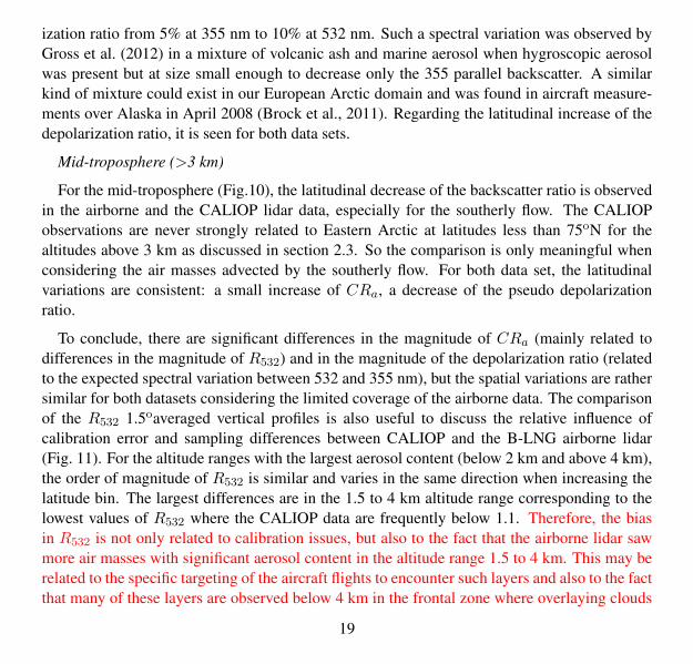
Mid-troposphere (>3 km)

For the mid-troposphere (Fig.10), the latitudinal decrease of the backscatter ratio is observedin the airborne and the CALIOP lidar data, especially for the southerly flow. The CALIOPobservations are never strongly related to Eastern Arctic at latitudes less than 75oN for thealtitudes above 3 km as discussed in section 2.3. So the comparison is only meaningful whenconsidering the air masses advected by the southerly flow. For both data set, the latitudinalvariations are consistent: a small increase of CRa, a decrease of the pseudo depolarizationratio.

To conclude, there are significant differences in the magnitude of CRa (mainly related todifferences in the magnitude of R532) and in the magnitude of the depolarization ratio (relatedto the expected spectral variation between 532 and 355 nm), but the spatial variations are rathersimilar for both datasets considering the limited coverage of the airborne data. The comparisonof the R532 1.5oaveraged vertical profiles is also useful to discuss the relative influence ofcalibration error and sampling differences between CALIOP and the B-LNG airborne lidar(Fig. 11). For the altitude ranges with the largest aerosol content (below 2 km and above 4 km),the order of magnitude of R532 is similar and varies in the same direction when increasing thelatitude bin. The largest differences are in the 1.5 to 4 km altitude range corresponding to thelowest values of R532 where the CALIOP data are frequently below 1.1. Therefore, the biasin R532 is not only related to calibration issues, but also to the fact that the airborne lidar sawmore air masses with significant aerosol content in the altitude range 1.5 to 4 km. This may berelated to the specific targeting of the aircraft flights to encounter such layers and also to the factthat many of these layers are observed below 4 km in the frontal zone where overlaying clouds

19

(see supplementary document) make more difficult a detection by the CALIOP overpasses. Thewider longitude range chosen for the CALIOP data set do not compensate for this difference inthe observed air masses. Since the difference in the magnitude of the 532 nm backscatter ratiois not only related to a calibration uncertainty in one instrument or both, but also to differencesin the number of observations with low aerosol content in the altitude range 1.5 to 4 km, wechoose not to apply any correction to the 532 nm CALIOP data set.

4 CALIOP characterization of the aerosol layer properties in April 2008

4.1 Latitudinal variability in the European Arctic

In this section, the CALIOP data are now analyzed for 30 days in April 2008 to improve fur-ther the signal-to-noise ratio. The latitudinal distribution of aerosol properties in the EuropeanArctic is still derived using average CALIOP vertical profiles for 1.5 olatitude bins, but over alarger domain between 65oN and 80oN. Two specific altitude ranges (0-2 km and 5-7 km) havebeen selected because they correspond to the largest aerosol load identified in the mean verticalprofile over the European Arctic (Fig.11).

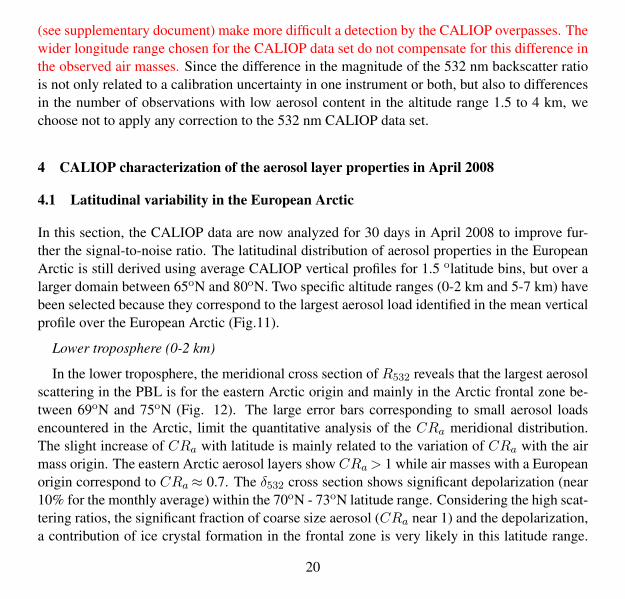
Lower troposphere (0-2 km)

In the lower troposphere, the meridional cross section of R532 reveals that the largest aerosolscattering in the PBL is for the eastern Arctic origin and mainly in the Arctic frontal zone be-tween 69oN and 75oN (Fig. 12). The large error bars corresponding to small aerosol loadsencountered in the Arctic, limit the quantitative analysis of the CRa meridional distribution.The slight increase of CRa with latitude is mainly related to the variation of CRa with the airmass origin. The eastern Arctic aerosol layers show CRa> 1 while air masses with a Europeanorigin correspond to CRa≈ 0.7. The δ532 cross section shows significant depolarization (near10% for the monthly average) within the 70oN - 73oN latitude range. Considering the high scat-tering ratios, the significant fraction of coarse size aerosol (CRa near 1) and the depolarization,a contribution of ice crystal formation in the frontal zone is very likely in this latitude range.

20

When excluding these specific cases, the European aerosol layers have larger depolarizationthan eastern Arctic air masses. Larger and more spherical aerosols for the eastern Arctic layersis not so surprising considering aerosol aging in air masses transported from Asia (Masslinget al., 2007).

Mid-troposphere (5-7 km)

In the mid troposphere (5-7km), there is a general decrease in R532 with latitude for theEuropean air masses, while it increases for the eastern Arctic origin. So in contrast to the PBLthere is a minimum of aerosol contribution near 72oN. This can be explained if one assumes asignificant wet removal of particles during upward vertical transport within the Arctic front. Asobserved for the lower troposphere, CRa values are lower for European air masses (near 0.5)than for Asian Arctic origin (near 0.8). We do not see the large depolarization values related tothe possible presence of ice crystals above 5 km, since they are not transported out of the PBL.However the meridional distribution of the depolarization shows a clear decrease at the highestlatitudes. The latitudinal increase of CRa associated with a decrease in depolarization couldbe explained by the increasing importance of aged anthropogenic aerosol and not to a stronginfluence of dust particles. The in-situ analysis of the size distribution made in Quennehenet al. (2012) indeed showed, that Asian anthropogenic aerosol contributed significantly to theaccumulation mode.

4.2 Large scale distribution in the Arctic domain

April monthly averages for R532, CRa and δ532 have been calculated for the complete Arcticdomain (latitude > 60oN) in horizontal boxes of 300 km x 300 km. The CRa values areonly given when R532>1.25 to focus on the contribution of significant aerosol plumes, and toavoid large errors in CRa due to small scattering ratios. The fraction of CALIOP observationsavailable (i.e. not below a cloud) in the selected altitude range is also given to estimate thenumber of effective CALIOP tracks in every box. According to Fig.1 a minimum number of 10overpasses is needed for the data to be representative of a monthly mean. This corresponds to afraction of 50% at 65oN and 20% at 80oN.

21

Lower troposphere (0-2 km)

In the lower troposphere (Fig. 13), theR532 map shows the extent of a North Atlantic aerosolcontribution with values remaining larger than 1.5 above 70oN. Sea salt and sulfate aerosol areknown to contribute to the increase of aerosol scattering over the Atlantic in winter and earlyspring (Smirnov et al., 2000; Yoon et al., 2007). The CRa map indicates a gradual increaseof CRa with latitude over North Atlantic: values < 0.7 occur near the mid-latitude sourceslocated below 65oN but CRa> 0.9 are frequent above 70oN. The latitudinal gradient of CRaover the North Atlantic ocean can be related to the growing influence of a different kind ofaerosol, since the probability of aerosol particle transport from the Eastern Arctic is increasingas discussed in the previous section. Aerosol composition analysis onboard the NOAA shipduring the ICEALOT campaign (Frossard et al., 2011) have shown that marine and sulfateaerosol represent 70% of the submicronic aerosol composition in the North Atlantic east ofIceland and they also found that the sulfate contribution increases with latitude. This is broadlyconsistent with the CALIOP observations.

A local maximum in the R532 map is also observed over Siberia between 90oE and 110oEwith a latitudinal extent up to 70oN in the Taymir peninsula. In Spring 2008 this area is knownto be influenced on one hand by local anthropogenic emissions from gas flaring (Stohl et al.,2013), and on the other hand by early spring forest fires in Russia (Warneke et al., 2010).The maximum in Northern Siberia is also seen for the same area in the AOD analysis madeby Winker et al. (2013) using CALIOP data for the winter period before the fire period, thenimplying a significant contribution of anthropogenic emissions. The CRa values < 0.7 aresimilar to those observed below 65oN over the Atlantic ocean. No significant depolarization isobserved in these two source regions implying very little impact from dust or volcano emissionsin this altitude range. The difference of CRa between European Arctic and the source region inRussia implies a growing of the aerosol particles during transport and aging if one assumes thatmost of the aerosol layers observed in European Arctic originate from Eurasia (see previoussection).

Mid-troposphere (5-7 km)

22

In the mid-troposphere (Fig. 14), the R532 map gives a very different picture of the linkbetween the Arctic aerosol distribution and the mid-latitude sources. There is first a broadaerosol maximum from eastern Siberia to western Alaska at latitudes between 60 oN and 75oNand second another maximum over the Hudson bay. The eastern Arctic domain north of 70oNis not as clean as in the lower troposphere, being consistent with an efficient transport pathwayfrom mid-latitudes along the tilted isentropic surfaces (Harrigan et al., 2011). The westernArctic and North Atlantic are relatively free of aerosol particles in the mid-troposphere. Thisis somewhat contradictory with the known uplift of the low level North American air pollutionover western Greenland (Harrigan et al., 2011; Ravetta et al., 2007). The contrast between thelarge aerosol concentrations found in the North Atlantic lower troposphere and the low valuesabove is also consistent with the conclusion of several papers (Law and Stohl, 2007; Harriganet al., 2011) about the transport pathway of European emission being most efficient in the lowertroposphere.

The global cloud distribution can be obtained from the DARDAR products, which are basedon CloudSat and CALIOP data according to a variational scheme, on a 60 m vertical resolutionand 1 km horizontal resolution grid (Delanoe and Hogan, 2008). The synergy between lidar andradar is indeed needed to have a detailed picture of the cloud vertical profile (Ceccaldi et al.,2013). It has been used here to calculate the cloud fraction at different altitudes during themonth of April 2008 in 4 different latitude bands from 60oN to 80oN (Fig. 15). The latitudeswith large cloudiness in both the mid and upper troposphere show upward frontal lifting byWarm Conveyor Belts (WCB) near the Bering strait and the western Greenland coast. Thelatter shows the largest cloudiness at 5 km. This may explain the low aerosol concentrationdownwind of Greenland due to efficient removal of aerosol. One can also notice the goodcorrelation between the high values of the low level cloud fraction and the large aerosol loadobserved above 70oN in the European Arctic.

The aerosol depolarization and color ratio distributions show small and little depolarization(except over the Hudson bay) in the large scale aerosol plumes seen in the mid-troposphere.However as in the lower troposphere, the CRa increase at latitudes >70oN is consistent withaerosol aging when reaching the highest latitudes.

23

5 Conclusions

In this paper we have analyzed aerosol airborne (B-LNG) and spaceborne (CALIOP) lidar datarelated to the transport of mid-latitude sources into the Arctic. The main results are the follow-ing:

– A campaign was held in April 2008 in the European Arctic with 18 aircraft cross sectionsand 80 CALIPSO tracks over 15 days improving our ability to identify the transport ofaerosol layers to the Arctic, especially from the analysis of the satellite data.

– Analysis of the B-LNG backscatter ratioR532 andR1064 at two wavelengths for the calcu-lation of the aerosol color ratio (CRa) has been successfully compared with in-situ aerosolmeasurements on-board the aircraft. The CRa increase corresponds to a similar increasein the mean aerosol diameter, showing the importance of multi-wavelength analysis. Italso emphasizes the need for accurate lidar calibration.

– Simulations with the FLEXPART model show that the limited number of airborne lidarcross sections are representative of the main characteristics of the air mass transport inApril 2008: increase with latitude of the aged air masses from the Eastern Arctic region ataltitude level below 3 km, large influence of the mid-latitudes sources directly transportedby the southerly flow at altitudes above 3 km.

– Comparisons are performed between B-LNG and CALIOP backscatter ratio R532 andR1064 at two wavelengths, including the calculation of the aerosol color ratio and of thedepolarization ratio (PDR) at 532 nm or 355 nm. Comparisons are based on the analysisof 15 day averages and L1 CALIOP data processing instead of AL2 CALIOP operationalproducts. Specific averaging methods can then be applied. The cloud screening, neededwhen using L1 lidar data, is based on CL2 CALIOP data products and the IR CALIPSOradiometer data. A re-calibration of the CALIOPR1064 in the Arctic was chosen to reducethe positive bias of the CALIOP data with respect to airborne observations of the colorratio. A fixed factor was applied to the 1064 nm attenuated backscatter data: respectively

24

1.3 and 1.4 for nighttime and daytime orbits. This value could be significatively smallerif a small negative bias of the 532 nm CALIOP lidar signal is also corrected. But thishypothesis was not chosen in this work. The use of the new V4.0 data which will becomeavailable very soon would certainly help to address this question.

– Comparisons of the statistical distributions in the altitude range 0-7 km show no sig-nificant bias for R1064 when correcting the CALIOP 1064 nm data but a -8% negativedifference between the CALIOP and B-LNG R532 data. The latter might be related to acalibration problem of either the B-LNG or the CALIOP instrument. However the differ-ences being largest in a specific altitude range between 1.5 and 4 km, differences of thespatial averaging of airborne and satellite data are also to be considered. The difference inthe magnitude of CRa is mainly related to this overestimate of R532 in the B-LNG data.The depolarization ratio is not measured at the same wavelength and its spectral variationfollows that of hygroscopic aerosol often at a size small enough to be detected only at355 nm (Gross et al., 2012).

– The latitudinal distribution of the color ratio and the depolarization ratio is similar for theB-LNG and the CALIOP data sets, especially considering the limited number of aircraftflights. It is a good indication that, despite possible bias in these two parameters whencomparing airborne and satellite data, they are still valuable for the analysis of the aerosolgrowth or the relative fraction of dust or volcanic ashes using CALIOP observations.

– The monthly average analysis of the CALIOP color and depolarization ratio in the Euro-pean Arctic area show that larger (higher CRa) and more spherical aerosol (low PDR)are expected in the air masses transported from the Eastern Arctic both in the lower tropo-sphere (0-2 km) and in the mid troposphere (5-7 km). Less aerosol is present in the midtroposphere near the arctic front (70oN-74oN) while significant R532 and depolarizationratio are seen in the lower troposphere possibly related to the presence of ice crystal.

– The global distribution of the CALIOP monthly analysis reveal two regions with largebackscatter below 2 km: the Northern Atlantic between Greenland and Norway, and the

25

Taymir peninsula. The CRa increase between the source regions and the observations atlatitudes above 70oN implies a growth of the aerosol size once transported to the Arctic.The distribution of the aerosol optical properties in the mid troposphere is consistent withthe transport pathways proposed in Harrigan et al. (2011): (i) low level advection in North-ern Europe (ii) isentropic uplifting of pollution and biomass burning aerosol in NorthernSiberia and Eastern Asia, (iii) aerosol washout by the North Atlantic warm conveyor belts.

Acknowledgements. The UMS SAFIRE is acknowledged for supporting the ATR-42 aircraft deploymentand for providing the aircraft meteorological data. The POLARCAT-FRANCE and CLIMSLIP projectswere funded by ANR, CNES, CNRS/INSU and IPEV. The FLEXPART team (A. Stohl, P. Seibert, A.Frank, G. Wotawa, C. Forster, S. Eckhardt, J. Burkhart, H. Sodemann) is acknowledged for providingthe FLEXPART code. NASA, CNES, the ICARE and LARC data center are gratefully acknowledge forsupplying the CALIPSO data.

References

Adam de Villiers, R., Ancellet, G., Pelon, J., Quennehen, B., Schwarzenboeck, A., Gayet, J. F., andLaw, K. S.: Airborne measurements of aerosol optical properties related to early spring transportof mid-latitude sources into the Arctic, Atmospheric Chemistry and Physics, 10, 5011–5030, doi:10.5194/acp-10-5011-2010, http://www.atmos-chem-phys.net/10/5011/2010/, 2010.

Brock, C. A., Cozic, J., Bahreini, R., Froyd, K. D., Middlebrook, A. M., McComiskey, A., Brioude,J., Cooper, O. R., Stohl, A., Aikin, K. C., de Gouw, J. A., Fahey, D. W., Ferrare, R. A., Gao, R.-S.,Gore, W., Holloway, J. S., Hubler, G., Jefferson, A., Lack, D. A., Lance, S., Moore, R. H., Murphy,D. M., Nenes, A., Novelli, P. C., Nowak, J. B., Ogren, J. A., Peischl, J., Pierce, R. B., Pilewskie, P.,Quinn, P. K., Ryerson, T. B., Schmidt, K. S., Schwarz, J. P., Sodemann, H., Spackman, J. R., Stark,H., Thomson, D. S., Thornberry, T., Veres, P., Watts, L. A., Warneke, C., and Wollny, A. G.: Charac-teristics, sources, and transport of aerosols measured in spring 2008 during the aerosol, radiation, andcloud processes affecting Arctic Climate (ARCPAC) Project, Atmospheric Chemistry and Physics, 11,2423–2453, doi:10.5194/acp-11-2423-2011, http://www.atmos-chem-phys.net/11/2423/2011/, 2011.

Burton, S. P., Ferrare, R. A., Hostetler, C. A., Hair, J. W., Rogers, R. R., Obland, M. D., Butler, C. F.,Cook, A. L., Harper, D. B., and Froyd, K. D.: Aerosol classification using airborne High Spectral

26

Resolution Lidar measurements - methodology and examples, Atmospheric Measurement Techniques,5, 73–98, doi:10.5194/amt-5-73-2012, http://www.atmos-meas-tech.net/5/73/2012/, 2012.

Cattrall, C., Reagan, J., Thome, K., and Dubovik, O.: Variability of aerosol and spectral lidar andbackscatter and extinction ratios of key aerosol types derived from selected Aerosol Robotic Networklocations, J. Geophys. Res., 110, D10S11, doi:10.1029/2004JD005124, 2005.

Ceccaldi, M., Delanoe, J., Hogan, R. J., Pounder, N. L., Protat, A., and Pelon, J.: From CloudSat-CALIPSO to EarthCare: Evolution of the DARDAR cloud classification and its comparison to air-borne radar-lidar observations, Journal of Geophysical Research: Atmospheres, 118, 7962–7981, doi:10.1002/jgrd.50579, http://dx.doi.org/10.1002/jgrd.50579, 2013.

Delanoe, J. and Hogan, R. J.: A variational scheme for retrieving ice cloud properties from combinedradar, lidar, and infrared radiometer, J. Geophys. Res., 113, D07 204, doi:10.1029/2007JD009000,2008.

Devasthale, A., Tjernstrm, M., Karlsson, K.-G., Thomas, M. A., Jones, C., Sedlar, J., and Omar, A. H.:The vertical distribution of thin features over the Arctic analysed from CALIPSO observations, TellusB, 63, 77–85, doi:10.1111/j.1600-0889.2010.00516.x, http://dx.doi.org/10.1111/j.1600-0889.2010.00516.x, 2011.

Di Pierro, M., Jaegle, L., Eloranta, E. W., and Sharma, S.: Spatial and seasonal distribution of Arc-tic aerosols observed by the CALIOP satellite instrument (20062012), Atmospheric Chemistry andPhysics, 13, 7075–7095, doi:10.5194/acp-13-7075-2013, http://www.atmos-chem-phys.net/13/7075/2013/, 2013.

Dubuisson, P., Giraud, V., Pelon, J., Cadet, B., and Yang, P.: Sensitivity of Thermal Infrared Radiationat the Top of the Atmosphere and the Surface to Ice Cloud Microphysics, Journal of Applied Mete-orology and Climatology, 47, 2545–2560, doi:10.1175/2008JAMC1805.1, http://dx.doi.org/10.1175/2008JAMC1805.1, 2008.

Freudenthaler, V., Esselborn, M., Wiegner, M., Heese, B., Tesche, M., Ansmann, A., Muller, D., Al-thausen, D., Wirth, M., Fix, A., Ehret, G., Knippertz, P., Toledano, C., Gasteiger, J., Garham-mer, M., and Seefeldner, M.: Depolarization ratio profiling at several wavelengths in pure Sa-haran dust during SAMUM 2006, Tellus, 61B, 165–179, doi:10.1111/j.1600-0889.2008.00396.x,http://dx.doi.org/10.1111/j.1600-0889.2008.00396.x, 2009.

Frossard, A. A., Shaw, P. M., Russell, L. M., Kroll, J. H., Canagaratna, M. R., Worsnop, D. R., Quinn,P. K., and Bates, T. S.: Springtime Arctic haze contributions of submicron organic particles from Eu-ropean and Asian combustion sources, Journal of Geophysical Research: Atmospheres, 116, DO5205,doi:10.1029/2010JD015178, http://dx.doi.org/10.1029/2010JD015178, 2011.

27

Fuelberg, H. E., Harrigan, D. L., and Sessions, W.: A meteorological overview of the ARCTAS 2008mission, Atmospheric Chemistry and Physics, 10, 817–842, doi:10.5194/acp-10-817-2010, http://www.atmos-chem-phys.net/10/817/2010/, 2010.

Garnier, A., Pelon, J., Dubuisson, P., Faivre, M., Chomette, O., Pascal, N., and Kratz, D. P.: Re-trieval of cloud properties using CALIPSO Imaging Infrared Radiometer. Part I: effective emis-sivity and optical depth, Journal of Applied Meteorology and Climatology, 51, 1407–1425, doi:10.1175/JAMC-D-11-0220.1, 2012.

Garrett, T. and Zhao, C.: Increased Arctic cloud longwave emissivity associated with pollution frommid-latitudes, Nature, 440, 787–789, 2006.

Gross, S., Freudenthaler, V., Wiegner, M., Gasteiger, J., Geiss, A., and Schnell, F.: Dual-wavelengthlinear depolarization ratio of volcanic aerosols: Lidar measurements of the Eyjafjallajkull plume overMaisach, Germany, Atmospheric Environment, 48, 85 – 96, doi:10.1016/j.atmosenv.2011.06.017,http://www.sciencedirect.com/science/article/pii/S1352231011006108, 2012.

Harrigan, D. L., Fuelberg, H. E., Simpson, I. J., Blake, D. R., Carmichael, G. R., and Diskin, G. S.:Anthropogenic emissions during Arctas-A: mean transport characteristics and regional case studies,Atmospheric Chemistry and Physics, 11, 8677–8701, doi:10.5194/acp-11-8677-2011, http://www.atmos-chem-phys.net/11/8677/2011/, 2011.

Jacob, D. J., Crawford, J. H., Maring, H., Clarke, A. D., Dibb, J. E., Emmons, L. K., Ferrare, R. A.,Hostetler, C. A., Russell, P. B., Singh, H. B., Thompson, A. M., Shaw, G. E., McCauley, E., Pederson,J. R., and Fisher, J. A.: The Arctic Research of the Composition of the Troposphere from Aircraftand Satellites (ARCTAS) mission: design, execution, and first results, Atmospheric Chemistry andPhysics, 10, 5191–5212, doi:10.5194/acp-10-5191-2010, http://www.atmos-chem-phys.net/10/5191/2010/, 2010.

Law, K. and Stohl, A.: Arctic Air Pollution: Origins and Impacts, Science, 315(5818), 1537–1540, doi10.1126/science.1137 695, 2007.

Liu, Z., Vaughan, M., Winker, D., Kittaka, C., Getzewich, B., Kuehn, R., Omar, A., Powell, K.,Trepte, C., and Hostetlerd, C.: The CALIPSO Lidar Cloud and Aerosol Discrimination: Version2 Algorithm and Initial Assessment of Performance, J. Atmos. Ocean. Tech., 26, 1198–1213, doi:10.1175/2009JTECHA1229.1, 2009.

Massling, A., Leinert, S., Wiedensohler, A., and Covert, D.: Hygroscopic growth of sub-micrometer andone-micrometer aerosol particles measured during ACE-Asia, Atmospheric Chemistry and Physics,7, 3249–3259, doi:10.5194/acp-7-3249-2007, http://www.atmos-chem-phys.net/7/3249/2007/, 2007.

Omar, A., Winker, D., Kittaka, C., Vaughan, M., Liu, Z., Hu, Y., Trepte, C., Rogers, R., Ferrare, R.,

28

Lee, K., Kuehn, R., and Hostetler, C.: The CALIPSO Automated Aerosol Classification and LidarRatio Selection Algorithm, J. Atmos. Ocean. Tech., 26, 1994–2014, doi:10.1175/2009JTECHA1231.1, 2009.

Powell, K. A., Hostetler, C. A., Vaughan, M. A., Lee, K.-P., Trepte, C. R., Rogers, R. R., Winker, D. M.,Liu, Z., Kuehn, R. E., Hunt, W. H., and Young, S. A.: CALIPSO Lidar Calibration Algorithms. Part I:Nighttime 532-nm Parallel Channel and 532-nm Perpendicular Channel, J. Atmos. Oceanic Technol.,26, 2015–2033, doi:10.1175/2009JTECHA1242.1, http://dx.doi.org/10.1175/2009JTECHA1242.1,2009.

Quennehen, B., Schwarzenboeck, A., Matsuki, A., Burkhart, J. F., Stohl, A., Ancellet, G., and Law,K. S.: Anthropogenic and forest fire pollution aerosol transported to the Arctic: observations fromthe POLARCAT-France spring campaign, Atmospheric Chemistry and Physics, 12, 6437–6454, doi:10.5194/acp-12-6437-2012, http://www.atmos-chem-phys.net/12/6437/2012/, 2012.

Quinn, P. K., Bates, T. S., Baum, E., Doubleday, N., Fiore, A. M., Flanner, M., Fridlind, A., Garrett,T. J., Koch, D., Menon, S., Shindell, D., Stohl, A., and Warren, S. G.: Short-lived pollutants in theArctic: their climate impact and possible mitigation strategies, Atmospheric Chemistry and Physics,8, 1723–1735, http://www.atmos-chem-phys.net/8/1723/2008/, 2008.

Rahn, K. A.: Relative importances of North America and Eurasia as sources of arctic aerosol, Atmo-spheric Environment, 15, 1447 – 1455, doi:10.1016/0004-6981(81)90351-6, 1981.

Ravetta, F., Ancellet, G., Colette, A., and Schlager, H.: Long Range Transport and Tropospheric OzoneVariability in Western Mediterranean Region during ITOP2004, J. Geophys. Res., 12, D10S46, doi:10.1029/2006JD007724, 2007.

Reagan, J., Wang, X., and Osborn, M. T.: Spaceborne lidar calibration from cirrus and molecularbackscatter returns, Geoscience and Remote Sensing, IEEE Transactions on, 40, 2285–2290, doi:10.1109/TGRS.2002.802464, 2002.

Rodrıguez, E., Toledano, C., Cachorro, V. E., Ortiz, P., Stebel, K., Berjon, A., Blindheim, S., Gausa, M.,and de Frutos, A. M.: Aerosol characterization at the sub-Arctic site Andenes (69oN, 16oE), by theanalysis of columnar optical properties, Quarterly Journal of the Royal Meteorological Society, 138,471–482, doi:10.1002/qj.921, http://dx.doi.org/10.1002/qj.921, 2012.

Rogers, R. R., Hostetler, C. A., Hair, J. W., Ferrare, R. A., Liu, Z., Obland, M. D., Harper, D. B.,Cook, A. L., Powell, K. A., Vaughan, M. A., and Winker, D. M.: Assessment of the CALIPSO Lidar532 nm attenuated backscatter calibration using the NASA LaRC airborne High Spectral ResolutionLidar, Atmospheric Chemistry and Physics, 11, 1295–1311, doi:10.5194/acp-11-1295-2011, http://www.atmos-chem-phys.net/11/1295/2011/, 2011.

29

Shinozuka, Y., Redemann, J., Livingston, J. M., Russell, P. B., Clarke, A. D., Howell, S. G., Fre-itag, S., O’Neill, N. T., Reid, E. A., Johnson, R., Ramachandran, S., McNaughton, C. S., Ka-pustin, V. N., Brekhovskikh, V., Holben, B. N., and McArthur, L. J. B.: Airborne observationof aerosol optical depth during ARCTAS: vertical profiles, inter-comparison and fine-mode frac-tion, Atmospheric Chemistry and Physics, 11, 3673–3688, doi:10.5194/acp-11-3673-2011, http://www.atmos-chem-phys.net/11/3673/2011/, 2011.

Smirnov, A., Holben, B. N., Kaufman, Y. J., Dubovik, O., Eck, T. F., Slutsker, I., Pietras, C., andHalthore, R. N.: Optical Properties of Atmospheric Aerosol in Maritime Environments, Journal ofthe Atmospheric Sciences, 59, 501–523, doi:10.1175/1520-0469(2002)059〈0501:OPOAAI〉2.0.CO;2, http://dx.doi.org/10.1175/1520-0469(2002)059〈0501:OPOAAI〉2.0.CO;2, 2000.

Stock, M., Ritter, C., Herber, A., von Hoyningen-Huene, W., Baibakov, K., Grser, J., Orgis, T., Tref-feisen, R., Zinoviev, N., Makshtas, A., and Dethloff, K.: Springtime Arctic aerosol: Smoke versushaze, a case study for March 2008, Atmospheric Environment, 52, 48–55, doi:10.1016/j.atmosenv.2011.06.051, http://www.sciencedirect.com/science/article/pii/S1352231011006637, 2011.

Stohl, A., Eckhardt, S., Forster, C., James, P., Spichtinger, N., and Seibert, P.: A replacement for simpleback trajectory calculations in the interpretation of atmospheric trace substance measurements,Atmospheric Environment, 36, 4635 – 4648, doi:10.1016/S1352-2310(02)00416-8, http://www.sciencedirect.com/science/article/B6VH3-46PBJBX-8/2/7d8c7b6557524176d31e8d96169cd1df,2002.

Stohl, A., Andrews, E., Burkhart, J. F., Forster, C., Herber, A., Hoch, S. W., Kowal, D., Lunder, C., Mef-ford, T., Ogren, J. A., Sharma, S., Spichtinger, N., Stebel, K., Stone, R., Strm, J., Trseth, K., Wehrli,C., and Yttri, K. E.: Pan-Arctic enhancements of light absorbing aerosol concentrations due to NorthAmerican boreal forest fires during summer 2004, Journal of Geophysical Research: Atmospheres,111, D22 214, doi:10.1029/2006JD007216, http://dx.doi.org/10.1029/2006JD007216, 2006.

Stohl, A., Klimont, Z., Eckhardt, S., Kupiainen, K., Shevchenko, V. P., Kopeikin, V. M., and Novigatsky,A. N.: Black carbon in the Arctic: the underestimated role of gas flaring and residential combus-tion emissions, Atmospheric Chemistry and Physics, 13, 8833–8855, doi:10.5194/acp-13-8833-2013,http://www.atmos-chem-phys.net/13/8833/2013/, 2013.

Vaughan, M. A., Powell, K. A., Winker, D. M., Hostetler, C. A., Kuehn, R. E., Hunt, W. H., Getzewich,B. J., Young, S. A., Liu, Z., and McGill, M. J.: Fully Automated Detection of Cloud and AerosolLayers in the CALIPSO Lidar Measurements, J. Atmos. Oceanic Technol., 26, 2034–2050, doi:10.1175/2009JTECHA1228.1, http://dx.doi.org/10.1175/2009JTECHA1228.1, 2009.

Vaughan, M. A., Liu, Z., McGill, M. J., Hu, Y., and Obland, M. D.: On the spectral dependence of

30

backscatter from cirrus clouds: Assessing CALIOP’s 1064 nm calibration assumptions using cloudphysics lidar measurements, Journal of Geophysical Research: Atmospheres, 115, D14 206, doi:10.1029/2009JD013086, http://dx.doi.org/10.1029/2009JD013086, 2010.

Vaughan, M. A., Garnier, A., Liu, Z., Josset, D., Hu, Y., Lee, K.-P., Hunt, W., Vernier, J.-P., Rodier,S., Pelon, J., and Winker, D.: Chaos, consternation and CALIPSO calibration: new strategies forcalibrating the CALIOP 1064 nm Channel, in: Proceedings of the 26th Int. Laser Radar Conf., PortoHeli, Greece, pp. 39–55, Alexandros Papayannis, University of Athens, Greece, 2012.

Vernier, J.-P., Pommereau, J.-P., Garnier, A., Pelon, J., Larsen, N., Nielsen, J., Christensen, T., Cairo,F., Thomason, L. W., Leblanc, T., and Mcdermid, I. S.: Tropical stratospheric aerosol layer fromCALIPSO lidar observations, Journal of Geophysical Research Atmospheres, 114, D00H10, doi:10.1029/2009JD011946, 2009.

Warneke, C., Froyd, K. D., Brioude, J., Bahreini, R., Brock, C. A., Cozic, J., de Gouw, J. A., Fahey,D. W., Ferrare, R., Holloway, J. S., Middlebrook, A. M., Miller, L., Montzka, S., Schwarz, J. P.,Sodemann, H., Spackman, J. R., and Stohl, A.: An important contribution to springtime Arctic aerosolfrom biomass burning in Russia, Geophys. Res. Lett., 37, L01 801, doi:10.1029/2009GL041816, http://dx.doi.org/10.1029/2009GL041816, 2010.

Winker, D. M., Vaughan, M. A., Omar, A., Hu, Y., Powell, K. A., Liu, Z., Hunt, W. H., andYoung, S. A.: Overview of the CALIPSO Mission and CALIOP Data Processing Algorithms, J. At-mos. Oceanic Technol., 26, 2310–2323, doi:10.1175/2009JTECHA1281.1, http://dx.doi.org/10.1175/2009JTECHA1281.1, 2009.

Winker, D. M., Tackett, J. L., Getzewich, B. J., Liu, Z., Vaughan, M. A., and Rogers, R. R.: The global3-D distribution of tropospheric aerosols as characterized by CALIOP, Atmospheric Chemistry andPhysics, 13, 3345–3361, doi:10.5194/acp-13-3345-2013, http://www.atmos-chem-phys.net/13/3345/2013/, 2013.

Wu, D. L., Chae, J. H., Lambert, A., and Zhang, F. F.: Characteristics of CALIOP attenuated backscatternoise: implication for cloud/aerosol detection, Atmospheric Chemistry and Physics, 11, 2641–2654,doi:10.5194/acp-11-2641-2011, http://www.atmos-chem-phys.net/11/2641/2011/, 2011.

Yoon, Y. J., Ceburnis, D., Cavalli, F., Jourdan, O., Putaud, J. P., Facchini, M. C., Decesari, S., Fuzzi,S., Sellegri, K., Jennings, S. G., and O’Dowd, C. D.: Seasonal characteristics of the physicochemicalproperties of North Atlantic marine atmospheric aerosols, Journal of Geophysical Research: Atmo-spheres, 112, D04 206, doi:10.1029/2005JD007044, http://dx.doi.org/10.1029/2005JD007044, 2007.

31

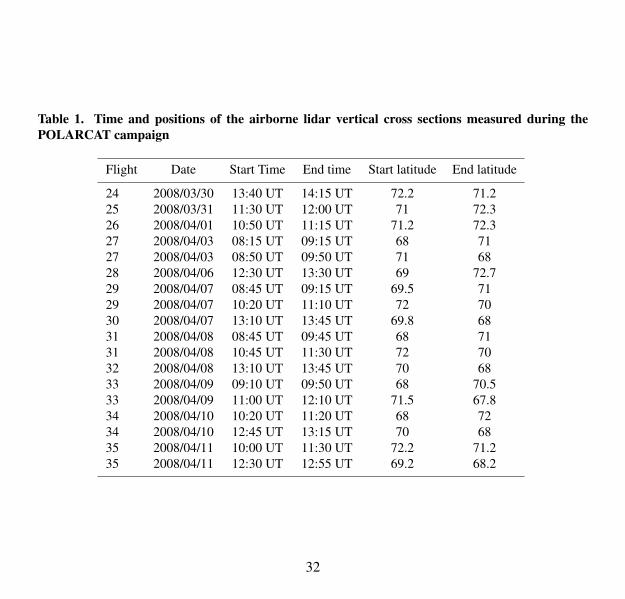
Table 1. Time and positions of the airborne lidar vertical cross sections measured during thePOLARCAT campaign

Flight Date Start Time End time Start latitude End latitude

24 2008/03/30 13:40 UT 14:15 UT 72.2 71.225 2008/03/31 11:30 UT 12:00 UT 71 72.326 2008/04/01 10:50 UT 11:15 UT 71.2 72.327 2008/04/03 08:15 UT 09:15 UT 68 7127 2008/04/03 08:50 UT 09:50 UT 71 6828 2008/04/06 12:30 UT 13:30 UT 69 72.729 2008/04/07 08:45 UT 09:15 UT 69.5 7129 2008/04/07 10:20 UT 11:10 UT 72 7030 2008/04/07 13:10 UT 13:45 UT 69.8 6831 2008/04/08 08:45 UT 09:45 UT 68 7131 2008/04/08 10:45 UT 11:30 UT 72 7032 2008/04/08 13:10 UT 13:45 UT 70 6833 2008/04/09 09:10 UT 09:50 UT 68 70.533 2008/04/09 11:00 UT 12:10 UT 71.5 67.834 2008/04/10 10:20 UT 11:20 UT 68 7234 2008/04/10 12:45 UT 13:15 UT 70 6835 2008/04/11 10:00 UT 11:30 UT 72.2 71.235 2008/04/11 12:30 UT 12:55 UT 69.2 68.2

32

Table 2. Comparison of mean aerosol layer pseudo (CR) and aerosol (CRa) color ratio measuredby the B-LNG lidar and in-situ measurements: CO mixing ratio, Grimm integral and CPC concen-trations, and the mean aerosol diameter from the SMPS+GRIMM spectrum. Layers with greenor yellow color are respectively for low or high value of CR.

Date Time (UT) lat.,dg alt. CO CR B-LNG CRa B-LNG CPC Grimm Dmeankm ppbv cm−3 cm−3 µm

30/03/08 13:45 72.0N 2.2 166 17.5±1.5% 38±6% 500 300 0.2207/04/08 09:05 70.3N 4.5 153 8.7±2% 39±64% 450 50 0.0708/04/08 11:20 70.7N 5.0 140 14.5±2.3% 62±44% 330 25 0.1308/04/08 13:12 69.9N 1.0 153 10.0±1.5% 19±6% 800 25 0.0708/04/08 13:17 69.7N 4.5 200 14.7±1.6% 27±6% 800 70 0.1608/04/08 13:50 68.4N 4.0 220 17.0±1.5% 28±4% 1000 150 0.1809/04/08 11:30 69.9N 4.5 210 10.0±1.8% 26±16% 2500 74 0.0707/04/08 10:15 69.0N 4.0 210 11.0±1.4% 19±5% 1000 50 0.1207/04/08 10:35 69.6N 3.5 230 18.7±1.5% 31±4% 900 300 0.2207/04/08 11:05 71.6N 3.5 200 17.0±1.6% 42±6% 700 250 0.18

33

//

Fig. 1. Aircraft trajectories for the measurement days listed in Table 1 (left) and positions of the CALIOPtracks from 27 March to 11 April (right).

34

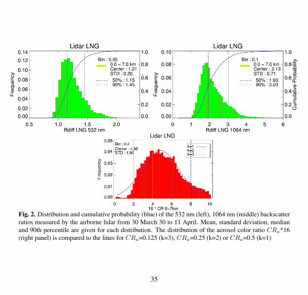
Fig. 2. Distribution and cumulative probability (blue) of the 532 nm (left), 1064 nm (middle) backscatterratios measured by the airborne lidar from 30 March 30 to 11 April. Mean, standard deviation, medianand 90th percentile are given for each distribution. The distribution of the aerosol color ratio CRa*16(right panel) is compared to the lines for CRa=0.125 (k=3), CRa=0.25 (k=2) or CRa=0.5 (k=1)

35

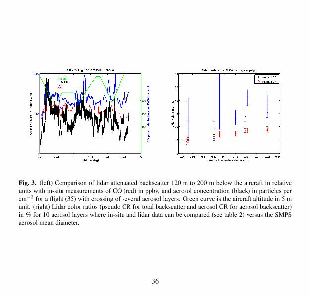
Fig. 3. (left) Comparison of lidar attenuated backscatter 120 m to 200 m below the aircraft in relativeunits with in-situ measurements of CO (red) in ppbv, and aerosol concentration (black) in particles percm−3 for a flight (35) with crossing of several aerosol layers. Green curve is the aircraft altitude in 5 munit. (right) Lidar color ratios (pseudo CR for total backscatter and aerosol CR for aerosol backscatter)in % for 10 aerosol layers where in-situ and lidar data can be compared (see table 2) versus the SMPSaerosol mean diameter.

36

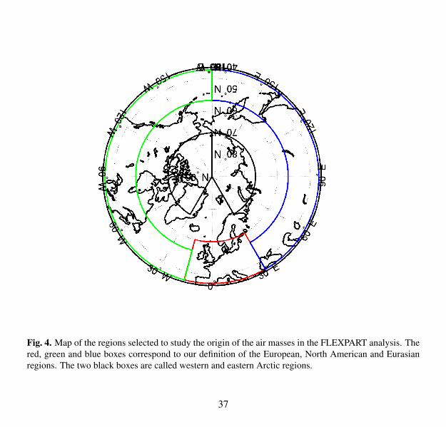
Fig. 4. Map of the regions selected to study the origin of the air masses in the FLEXPART analysis. Thered, green and blue boxes correspond to our definition of the European, North American and Eurasianregions. The two black boxes are called western and eastern Arctic regions.

37

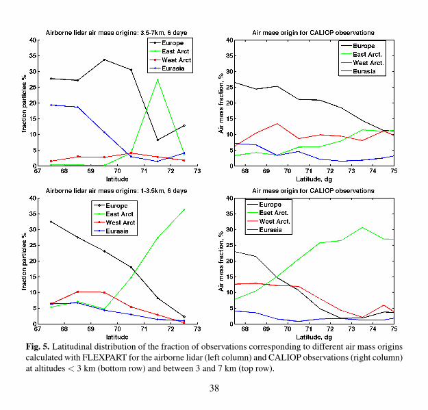
Fig. 5. Latitudinal distribution of the fraction of observations corresponding to different air mass originscalculated with FLEXPART for the airborne lidar (left column) and CALIOP observations (right column)at altitudes < 3 km (bottom row) and between 3 and 7 km (top row).

38

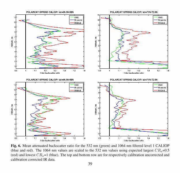
Fig. 6. Mean attenuated backscatter ratio for the 532 nm (green) and 1064 nm filtered level 1 CALIOP(blue and red). The 1064 nm values are scaled to the 532 nm values using expected largest CRa=0.5(red) and lowest CRa=1 (blue). The top and bottom row are for respectively calibration uncorrected andcalibration corrected IR data.

39

Fig. 7. Correlation between the 532 nm and 1064 nm mean backscatter ratio measured by filtered level1 CALIOP from 27 March to 11 April 2008, at altitudes from 0 to 7 km (top row) and 13 to 15 km(bottom row) using either uncorrected (left) or corrected (right) IR backscatter data. Regression line isthe dashed-dotted blue line. The lines k=-1, 0, 1 are respectively for tropospheric aerosol distributionwith CRa=2, 1, 0.5..

40

Fig. 8. Distribution of the 532 nm (left), 1064 nm (middle) backscatter ratios from filtered level 1CALIOP data at altitudes from 0 to 7 km (green) and 13 to 15 km (red) from 27 March to 11 April in theaircraft flight area. Mean, standard deviation, median and 90th percentile are given for each distribution.The maximum of the aerosol color ratio 16*CRa distribution (right panel) is compared to the lines forCRa=0.125 (k=3), CRa=0.25 (k=2) or CRa=0.5 (k=1)

41

Fig. 9. Latitudinal distribution of 532 nm backscatter ratio (left), aerosol color ratio (middle) and pseudodepolarization ratio (right) for the airborne lidar observations (top) and filtered level 1 CALIOP (bottom)at altitudes < 3 km during the aircraft campaign. The colors are for different air mass origins estimatedwith Flexpart (see text).

42

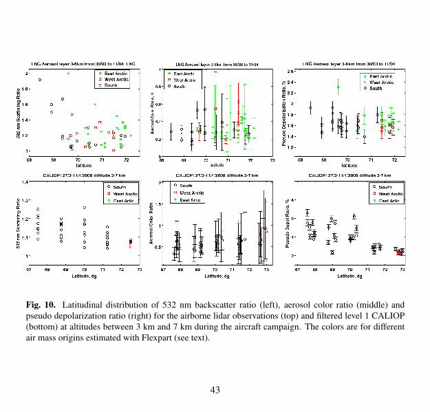
Fig. 10. Latitudinal distribution of 532 nm backscatter ratio (left), aerosol color ratio (middle) andpseudo depolarization ratio (right) for the airborne lidar observations (top) and filtered level 1 CALIOP(bottom) at altitudes between 3 km and 7 km during the aircraft campaign. The colors are for differentair mass origins estimated with Flexpart (see text).

43

Fig. 11. Mean 532-nm backscatter ratio vertical profile over a 1.5 olatitude band for the airborne lidardata (left) and filtered level 1 CALIOP data (right)

44

Fig. 12. Latitudinal distribution of 532 nm backscatter ratio (left), aerosol color ratio (middle) and pseudodepolarization ratio (right) for filtered level 1 CALIOP in April 2008 at altitudes < 2 km (bottom) andbetween 5 km and 7 km (top). The origin of the layers are estimated with Flexpart (see text).

45

Fig. 13. Map of the 532 nm backscatter ratio, aerosol color ratio, pseudo depolarization ratio and fractionof cloudless observations using the April 2008 filtered level 1 CALIOP data in the 0-2 km altitude range.

46

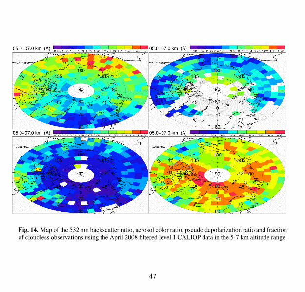
Fig. 14. Map of the 532 nm backscatter ratio, aerosol color ratio, pseudo depolarization ratio and fractionof cloudless observations using the April 2008 filtered level 1 CALIOP data in the 5-7 km altitude range.

47

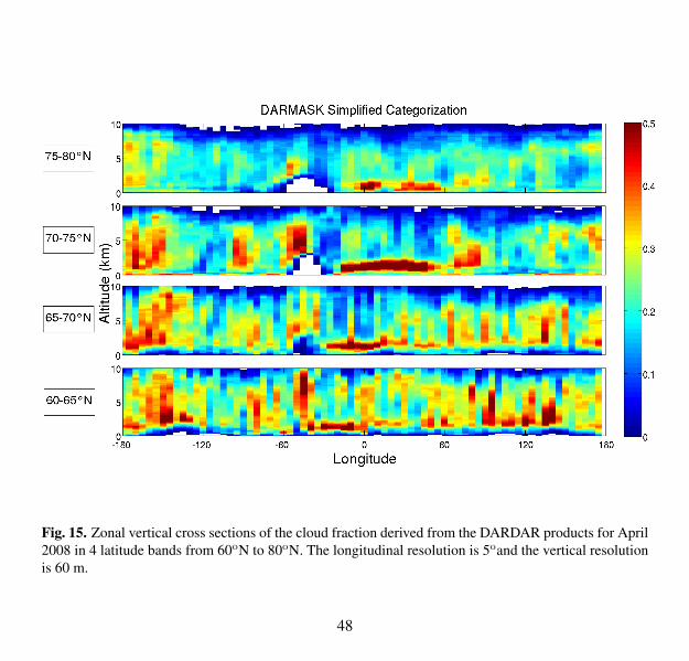
Fig. 15. Zonal vertical cross sections of the cloud fraction derived from the DARDAR products for April2008 in 4 latitude bands from 60oN to 80oN. The longitudinal resolution is 5oand the vertical resolutionis 60 m.

48