Lecture 15: Two special modes for AFM: Electrostatic Force Microscopy (EFM) and Magnetic Force Microscopy (MFM)

• basic principles and mechanisms of EFM and MFM; • two scanning modes; • typical applications: with EFM for applications in interfacial charge transfer and separation, and MFM for exploring the nanostructural magnetic information's (real case studies as inspired from mother Nature).

EFM also called: scanning electrostatic potential microscopy (SEPM) (Force feedback; potential measurement)

What is EFM?

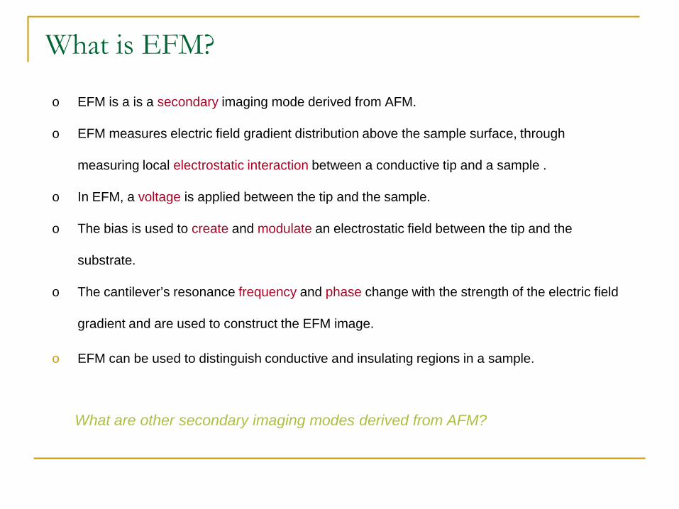
o EFM is a is a secondary imaging mode derived from AFM.

o EFM measures electric field gradient distribution above the sample surface, through

measuring local electrostatic interaction between a conductive tip and a sample .

o In EFM, a voltage is applied between the tip and the sample.

o The bias is used to create and modulate an electrostatic field between the tip and the

substrate.

o The cantilever’s resonance frequency and phase change with the strength of the electric field

gradient and are used to construct the EFM image.

o EFM can be used to distinguish conductive and insulating regions in a sample.

What are other secondary imaging modes derived from AFM?

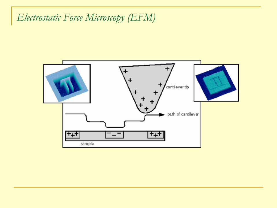
Electrostatic Force Microscopy (EFM)

Electrostatic Interaction Upon Voltage Application

100 µm

25 µm 3 µm

20 nm

bias = 1 V

Tip apex

Tip cone

Cantilever

Cantilever frequency change due to electrostatic interaction

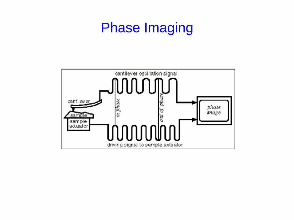
Phase Imaging

Two types of EFM measurement:

1. Lifted mode: constant height Because the electrostatic forces interact at greater distances than van der

Waals forces, so electrical force information can be separated from surface topography simply by increseasing the tip-to-sample distance --- lift up the tip.

Dual scanning --- Grounded tip first acquires surface topography in the tapping mode, then the tip is lifted up, and retraces the surface profile maintaining constant tip-surface separation.

During the second scan, tip is no longer driven mechanically by the piezoactuator --- no feedback required, faster scanning available.

A constant voltage is maintained on the tip. As the tip moves over an attractive electric field gradient, it is pulled toward the sample. When the tip traverses a repulsive gradient, it is pushed away from the sample.

The deflection (or frequency change) of the cantilever, proportional to the charge density, can be measured using the standard light-lever system.

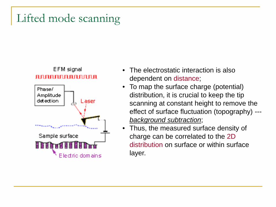
Lifted mode scanning

• The electrostatic interaction is also dependent on distance;

• To map the surface charge (potential) distribution, it is crucial to keep the tip scanning at constant height to remove the effect of surface fluctuation (topography) --- background subtraction;

• Thus, the measured surface density of charge can be correlated to the 2D distribution on surface or within surface layer.

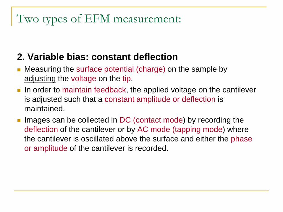
Two types of EFM measurement:

2. Variable bias: constant deflection Measuring the surface potential (charge) on the sample by

adjusting the voltage on the tip. In order to maintain feedback, the applied voltage on the cantilever

is adjusted such that a constant amplitude or deflection is maintained.

Images can be collected in DC (contact mode) by recording the deflection of the cantilever or by AC mode (tapping mode) where the cantilever is oscillated above the surface and either the phase or amplitude of the cantilever is recorded.

Bias modulated feedback

Bias

modulation all

interactions

Only van der Waals

force

Total force between tip and sample

Total force = capacitive force + Coulomb interaction + van der Waals force + hard-sphere repulsion.

• C is the tip-sample capacitance; • Vb is the bias voltage applied to the sample, • ϕ is the surface potential difference between the tip and substrate, • Ez is the static field due to charges or multipoles of the sample excluding the field of charges

accumulated on capacitor plates, namely, the tip and the substrate under bias voltages. • FVDW is the van der Waals force, • Fhs is the hard-sphere repulsion when the tip and the sample are in very close contact,

small

When applied bias Vb = - ϕ, all electrostatic interactions are nullified.

Typical applications of EFM

characterizing surface electrical properties;

electronic properties of nanocrystals (trap sites, charge storage, etc.);

Interfacial charge transport and separation for organic/electrode devices

(conducting polymer, organic semiconductors, etc.);

detecting defects of an integrated circuit (silicon surface);

measuring the distribution of a particular material on a composite

surface.

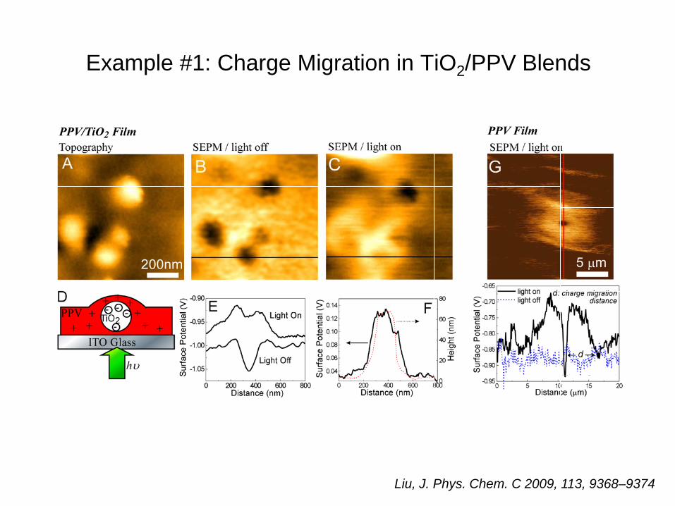
Example #1: Charge Migration in TiO2/PPV Blends

Liu, J. Phys. Chem. C 2009, 113, 9368–9374

Example #2: Charge re-distribution and Fermi level pinning at organic/inorganic interface

Liwei Chen, L. Brus, et al. J. Phys. Chem. B 2005, 109, 1834-1838

• For many organic semiconductors devices like TFT, LED, LCD, solar cells, interfacial charge transfer (electrode injection) represents the ultimate step in transport processes of charge carriers.

• The efficiency of interfacial charge transfer and/or separation determines the overall performance of the devices.

• EFM measurements provide direct mapping of the local charge density at high spatial resolution.

• Here the material used is pentacene, one of the most popular organic semiconductors, which has high charge mobility ~ 1 cm2 V-1 s-1, and high gate modulation of current, 107 – 108.

Liwei Chen, L. Brus, et al. J. Phys. Chem. B 2005, 109, 1834-1838

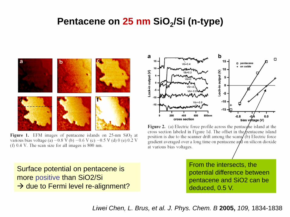
Pentacene on 25 nm SiO2/Si (n-type)

From the intersects, the potential difference between pentacene and SiO2 can be deduced, 0.5 V.

Surface potential on pentacene is more positive than SiO2/Si due to Fermi level re-alignment?

Example #3: Interfacial charge transfer of nanocrystals

Oksana Cherniavskaya, L. Brus, et al. J. Phys. Chem. B 2004, 108, 4946-4961

• Nanoparticle: a transition manifestation between molecules and bulk

materials;

• Size-tunable physical and chemical properties;

• Large ratio of surface atoms --- defects density upon surface modification;

• Thus vast applications in optical and electronic devices;

• Interfacial charge transfer is crucial for understanding and designing

nanocrystal based devices.

• Detailed modeling and theoretical analysis of EFM measurement can be found in the

following paper.

Tuning bandgap (i.e. λem): Quantum Size Effect

(Particle size)

CdSe

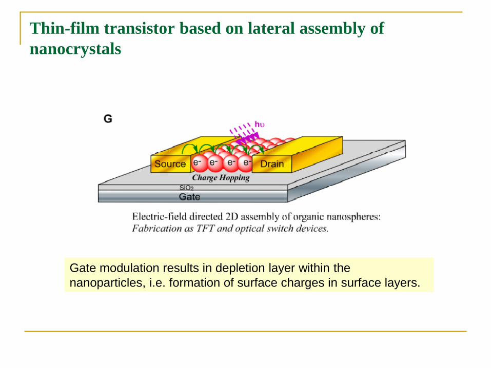
Thin-film transistor based on lateral assembly of nanocrystals

Gate modulation results in depletion layer within the nanoparticles, i.e. formation of surface charges in surface layers.

Oksana Cherniavskaya, L. Brus, et al. J. Phys. Chem. B 2004, 108, 4946-4961

Example #3: Interfacial charge transfer of nanocrystals: EFM measurement

J. Phys. Chem. B 2004, 108, 4946-4961

CdSe/CdS nanocrystals on n-type silicon under illumination

Before illumination upon illumination

• Before exposure to light, there is only one nanoparticle showing a charge signal.

• Once exposed to light, many charged particles appear. • Equilibrium is reached around 100 min.

Example #4: Charge separation between semiconductor-metal nanoparticle: implication for a variety of applications in optoelectronic devices.

Nano Lett., 2009, 9 (5), pp 2031–2039

Electrostatic Force Microscopy Study of Single Au−CdSe Hybrid Nanodumbbells (NDBs): Evidence for Light-Induced Charge Separation

(a) A scheme of the EFM setup used demonstrating a two pass scan of each line with bias application in the interleaved scan. (b) TEM image of hybrid CdSe-Au nanodumbbells used in this work. (c) AFM tapping mode topography image of nanodumbbells with the corresponding phase image (d) showing contrast difference between the gold tips (white arrows) and the CdSe rods.

Example #4: Charge separation between semiconductor-metal nanoparticle: implication for a variety of applications in optoelectronic devices.

Correlated tapping mode topography image (a) and charge images (ω) before (b) and during (c) irradiation of a sample of NDBs. The change in the signal between images b and c is indicative of negative charging of the NDBs while under irradiation. In comparison, a correlated tapping mode topography image (d) and charge images (ω) before (e) and during (f) irradiation of a sample of CdSe nanorods shows a positive charging behavior under irradiation. (Circles on some of the particles are shown as a guide to the eye).

No light light

Positive charge

negative charge

Example #4: Charge separation between semiconductor-metal nanoparticle: implication for a variety of applications in optoelectronic devices.

What is MFM?

MFM is a is a secondary imaging mode derived from Tapping-Mode AFM.

MFM images the spatial variation of magnetic field within the sample surface, through measuring local magnetic interaction between a conductive tip and a sample .

In MFM, a magnetic tip coated with a ferromagnetic thin film (e.g., CoCr or NiFe ) is used.

MFM detectes changes in the resonant frequency of the cantilever induced by the magnetic interaction with the sample surface.

The cantilever’s resonance frequency and phase change with the strength of the magnetic field gradient and are used to construct the MFM image.

MFM can be used to image both naturally occurring and deliberately written domain structures in magnetic materials.

Magnetic Force Microscopy (MFM)

MFM image of a hard disk (30 µm)

Dual scanning --- Lifted mode:

Because the magnetic forces interact at greater distances than van der Waals forces, so electrical or magnetic force information can be separated from surface topography simply by increseasing the tip-to-sample distance --- lift up the tip.

Dual scanning --- the tip first acquires surface topography in the tapping mode, then the tip is lifted up, and retraces the surface profile maintaining constant tip-surface separation.

During the second scan, tip is no longer driven mechanically by the piezoactuator --- no feedback required.

As the tip moves over an magnetic field gradient, it is either pulled toward or repulsed away from the sample, depending on the magnetic moment direction of the sample.

The deflection (or frequency change) of the cantilever, proportional to the magnetic field strength, can be measured using the standard light-lever system.

Lift-Mode --- a patented technique of DI. It separately measures topography and another selected property, like magnetic force (MFM), and electric force (EFM), using the topographical information to track the probe tip at a constant height (Lift Height) above the sample surface during the second scanning.

Lifted-mode scanning

Applications and advantages of MFM imaging

MFM can be used to evaluate magnetic materials and devices or to locate and map magnetic defects on a variety of materials and surfaces.

Applications of MFM imaging include:

1. data recording/storage media,

2. nanoparticles (e.g. biological separation and purification),

3. thin films,

4. detection of magnetic beads,

5. biological magnetic sensing (e.g. long migration of sea turtle and homing pigeon, next slide)

MFM brings the advantages of AFM into the magnetic materials.

MFM is non-destructive and requires minimal sample preparation.

MFM is compatible with imaging in fluids or in air, imaging under controlled environments (e.g. pressure, temperature).

Researches showed:

bird beaks contain small magnetic particles called magnetite.

Using magnetite, the birds are able to sense the Earth's magnetic fields that provide

information about location.

Homing pigeons can find their way home with ease. Pigeons Detect Magnetic Fields Nose Knows North (and South, West and East)

Nature, 2004, vol.432, pp508-511.

Case study #1:

Case study #1: Orientation and Navigation of Sea Turtles (nanoscopic magnetic sensor? --- to be explored by MFM?)

• As hatchlings, turtles that have never before been in the ocean are able to establish unerring courses towards the open sea and then maintain their headings cross the ocean;

• homing back to specific locations after long migrations.

Example #1: revealing nanoscale magnetic domain

Magnetic Force Microscopy (MFM) of a Magnetic Hard Disk

Example #2: Fabrication of New Generation of Hard Disk

• Conventional hard disks consist of sputtered magnetic thin films with single domain grains.

• The orientation of the magnetisation of these grains is randomly distributed in the plane of the medium.

• Some 100 grains are necessary to build one bit with a sufficient signal to noise ratio (S/N). The lateral size of a grain is typical 10 nm. Therefore the smallest allowable bit size is of the order of 100 x 100 nm2.

• The grain size may be reduced, but for grain sizes smaller than 7 nm the magnetisation of one grain will become thermal unstable (superparamagnetic).

• In summary, the storage density in conventional hard disk is therefore fundamentally limited. These limits are expected to have been reached soon.

Mesoscopic structure of hard disk

• A solution to break the density limit of conventional hard disk --- to pattern the

magnetic layer in a regular matrix of dots.

• In such a discrete recording medium, every dot represents one bit.

• One requirement --- these dots are single domain and have a strong uniaxial

magnetic anisotropy, so that only two well defined magnetisation states are

possible.

• It is obvious that a special patterning technique is required --- a large and

regularly patterned area of at least 50x50 nm2 sized dots with 100 nm period

can be obtained. See the slide.

• Also, for the recording of this type of media, new technologies have to be

developed.

New generation of hard disk

Laser Interference Lithography

Working principle of laser interference lithography, and examples of etched dot structure patterned with Laser Interference Lithography (period = 570 nm)

M.A.M. Haast et al., Journal of Magnetism and Magnetic Materials Vol. 193 1999 511-514

Magnetic Force Microscopy image of 70 nm single domain dots at 200 nm period

• The dots are in a single domain state with only two orientations, i.e. up and down;

• This meets the requirement for a patterned medium.

• The density of this medium is 16 GBit/In2, considerably higher than state-of-the-art hard disk technology.

(10 µm x 10µm) Magnetic Force Microscope scan of a 200nm thick cobalt crystal layer showing magnetic domains

Example #3 : High lateral resolution using sharp tip

Magnetic Force Microscopy image of a (111) surface of a Fe 3%Si single crystal, displaying a multi-scale domain structure (40x40µm²).

Example #4 : inhomogeneous magnetic domain in atomic homogeneous phase