1

Chapter 9A. Process Capability & Statistical Quality Control

Outline:Basic StatisticsProcess VariationProcess Capability Process Control Procedures

Variable data X-bar chart and R-chart

Attribute data p-chart

Acceptance Sampling Operating Characteristic Curve

2

Focus This technical note on statistical quality control (SQC)

covers the quantitative aspects of quality management SQC is a number of different techniques designed to

evaluate quality from a conformance view How are we doing in meeting specifications?

SQC can be applied to both manufacturing and service processes

SQC techniques usually involve periodic sampling of the process and analysis of data Sample size Number of samples

SQC techniques are looking for variance Most processes produce variance variance in output

we need to monitor the variance (and the mean also) and correct processes when they get out of range

Dr. Saydam, Lecture 1 3

Mean

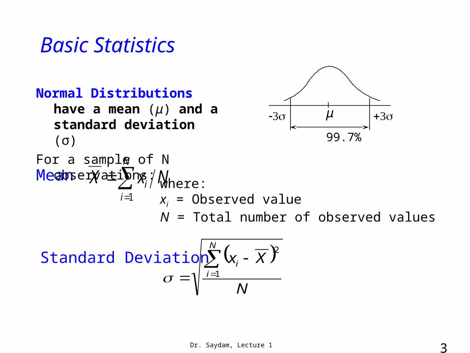
Basic Statistics

Normal Distributions have a mean (μ) and a standard deviation (σ)

For a sample of N observations:

N

ii NxX

1

N

XxN

ii

1

2

where:xi = Observed valueN = Total number of observed values

Standard Deviation

99.7%

μ

4

Statistics and Probability

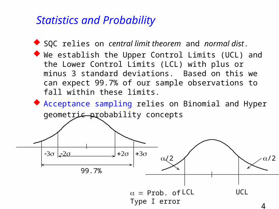
SQC relies on central limit theorem and normal dist. We establish the Upper Control Limits (UCL) and the

Lower Control Limits (LCL) with plus or minus 3 standard deviations. Based on this we can expect 99.7% of our sample observations to fall within these limits.

Acceptance sampling relies on Binomial and Hyper geometric probability concepts

99.7%

LCL UCL

/2 /2

Prob. ofType I error

Dr. Saydam, Lecture 1 5

Using SQC, samples of a process output are taken, and sample statistics are calculated

The purpose of sampling is to find when the process has changed in some nonrandom way The reason for the change can then be quickly

determined and corrected

This allows us to detect changesdetect changes in the actual distribution process

Basic Stats

6

Variation

Random (common) variation is inherent in the production process.

Assignable variation is caused by factors that can be clearly identified and possibly managed

Using a saw to cut 2.1 meter long boards as a sample process Discuss random vs. assignable variation

Generally, when variation is reduced, quality improves. It is impossible to have zero variability. T or F ?

Dr. Saydam, Lecture 1 7

IncrementalCost of Variability

High

Zero

LowerSpec

TargetSpec

UpperSpec

Traditional View

IncrementalCost of Variability

High

Zero

LowerSpec

TargetSpec

UpperSpec

Taguchi’s ViewExhibits TN8.1 & TN8.2

Exhibits TN8.1 & TN8.2

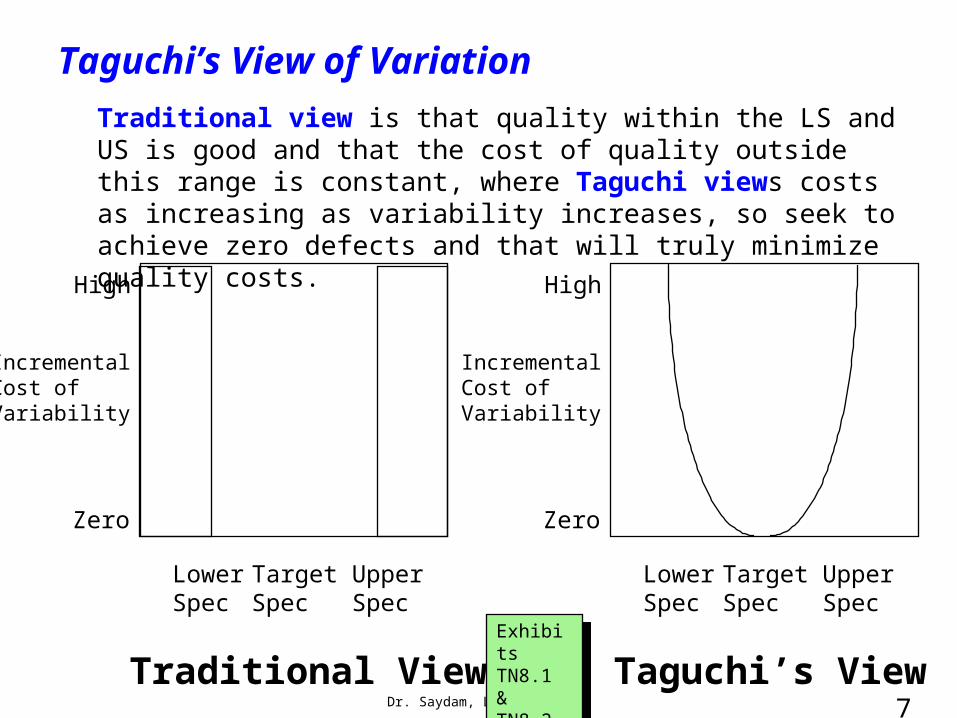
Taguchi’s View of VariationTraditional view is that quality within the LS and US is good and that the cost of quality outside this range is constant, where Taguchi views costs as increasing as variability increases, so seek to achieve zero defects and that will truly minimize quality costs.

Dr. Saydam, Lecture 1 8

Process Capability

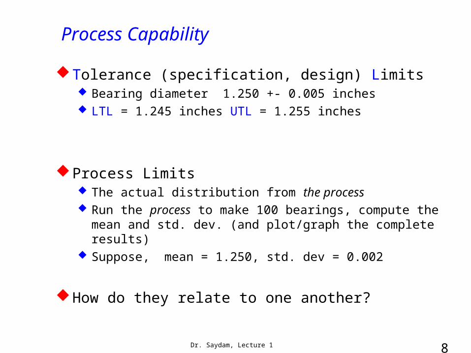
Tolerance (specification, design) Limits Bearing diameter 1.250 +- 0.005 inches LTL = 1.245 inches UTL = 1.255 inches

Process Limits The actual distribution from the process Run the process to make 100 bearings, compute the

mean and std. dev. (and plot/graph the complete results)

Suppose, mean = 1.250, std. dev = 0.002

How do they relate to one another?

9

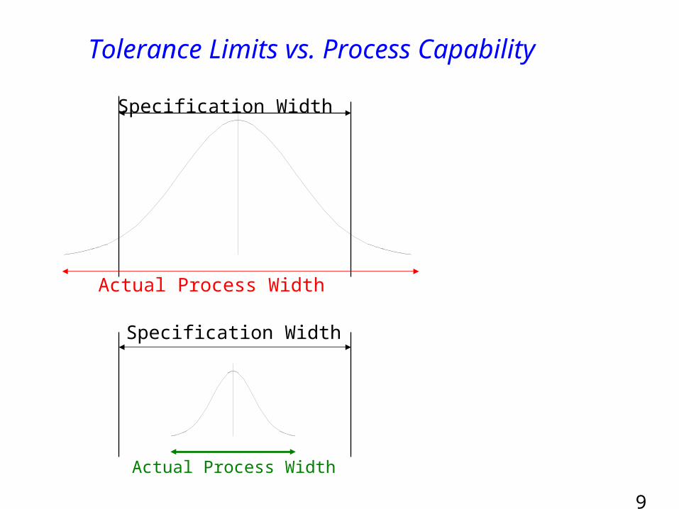
Tolerance Limits vs. Process Capability

Actual Process Width

Specification Width

Specification Width

Actual Process Width

10

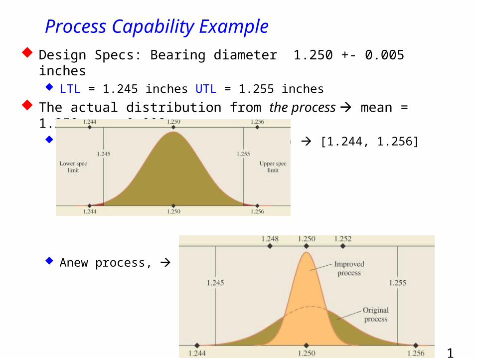
Process Capability Example Design Specs: Bearing diameter 1.250 +- 0.005 inches

LTL = 1.245 inches UTL = 1.255 inches The actual distribution from the process mean = 1.250, s

= 0.002 +- 3s limits 1.250 +- 3(0.002) [1.244, 1.256]

Anew process, std. dev. = 0.00083

11

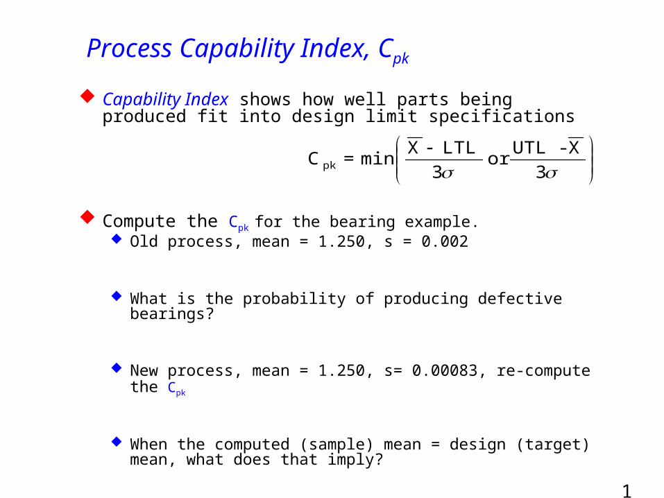
Process Capability Index, Cpk

Capability Index shows how well parts being produced fit into design limit specifications

Compute the Cpk for the bearing example. Old process, mean = 1.250, s = 0.002

What is the probability of producing defective bearings?

New process, mean = 1.250, s= 0.00083, re-compute the Cpk

When the computed (sample) mean = design (target) mean, what does that imply?

3

X-UTLor

3

LTLXmin=C pk

12

The Cereal Box Example

Recall the cereal example. Consumer Reports has just published an article that shows that we frequently have less than 15 ounces of cereal in a box.

Let’s assume that the government says that we must be within ± 5 percent of the weight advertised on the box.

Upper Tolerance Limit = 16 + 0.05(16) = 16.8 ounces Lower Tolerance Limit = 16 – 0.05(16) = 15.2 ounces

We go out and buy 1,000 boxes of cereal and find that they weight an average of 15.875 ounces with a standard deviation of 0.529 ounces.

13

Cereal Box Process Capability

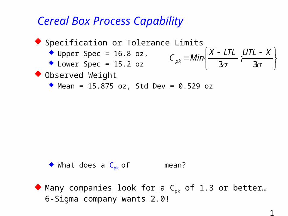
Specification or Tolerance Limits Upper Spec = 16.8 oz, Lower Spec = 15.2 oz

Observed Weight Mean = 15.875 oz, Std Dev = 0.529 oz

What does a Cpk of 0.4253 mean?

Many companies look for a Cpk of 1.3 or better… 6-Sigma company wants 2.0!

3

;3

XUTLLTLXMinC pk

14

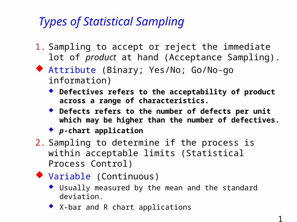
Types of Statistical Sampling

1. Sampling to accept or reject the immediate lot of product at hand (Acceptance Sampling).

Attribute (Binary; Yes/No; Go/No-go information) Defectives refers to the acceptability of product

across a range of characteristics. Defects refers to the number of defects per unit

which may be higher than the number of defectives.

p-chart application

2. Sampling to determine if the process is within acceptable limits (Statistical Process Control)

Variable (Continuous) Usually measured by the mean and the standard

deviation. X-bar and R chart applications

15

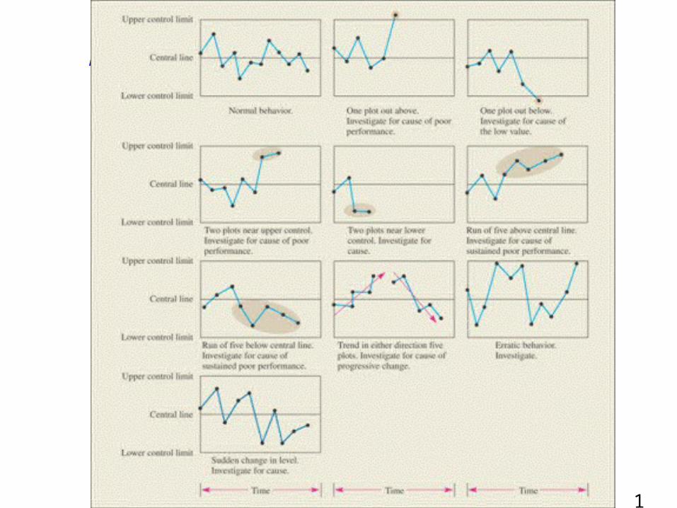
Evidence for Investigation…

16

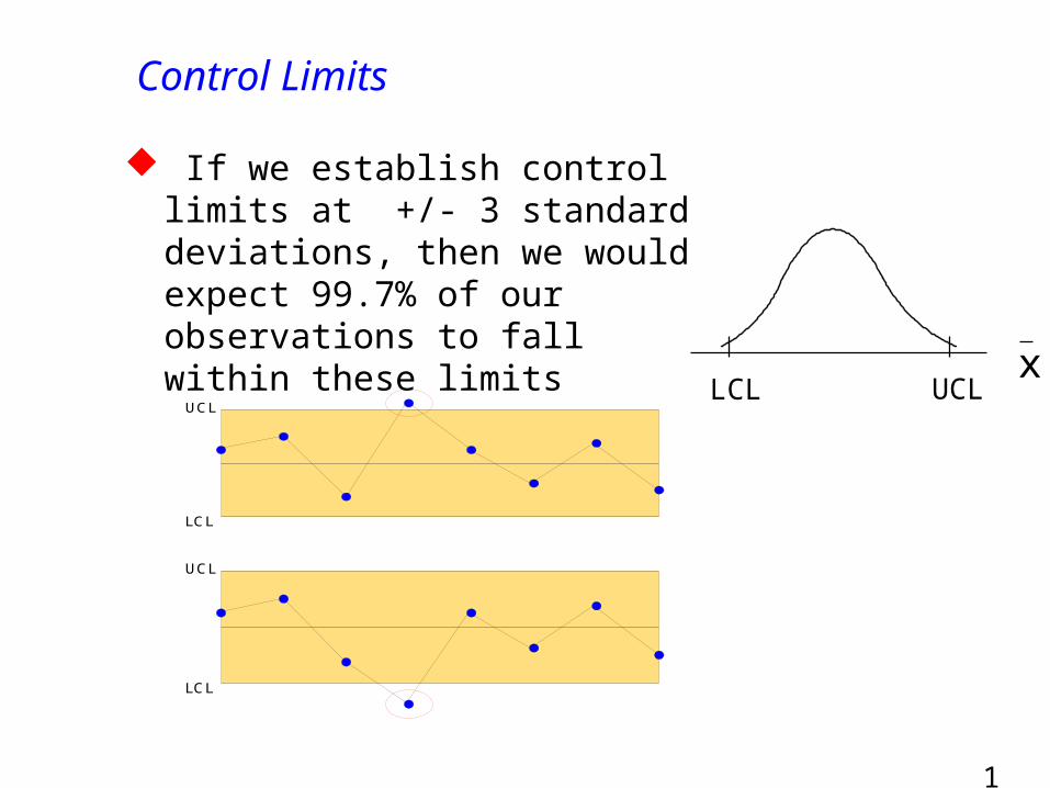
Control Limits

If we establish control limits at +/- 3 standard deviations, then we would expect 99.7% of our observations to fall within these limits

xLCL UCL

UCL

LCL

UCL

LCL

17

Attribute Measurements (p-Chart)

Item is “good” or “bad”Collect data, compute average fraction bad

(defective) and std. dev. using:

The, UCL, LCL using:

Excel time!

ns

)p-(1 p =

nsObservatio ofNumber Total

Defectives ofNumber Total=p

p

p

p

Z- p = LCL

Z p = UCL

s

s

18

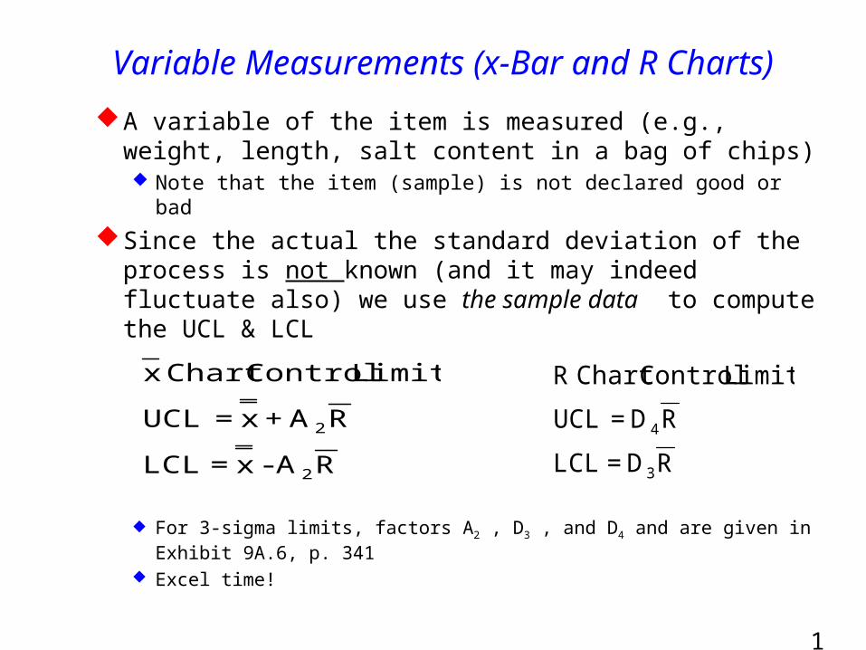
Variable Measurements (x-Bar and R Charts)A variable of the item is measured (e.g., weight, length, salt content in a bag of chips) Note that the item (sample) is not declared good or bad

Since the actual the standard deviation of the process is not known (and it may indeed fluctuate also) we use the sample data to compute the UCL & LCL

For 3-sigma limits, factors A2 , D3 , and D4 and are given in Exhibit 9A.6, p. 341

Excel time!

RA - x = LCL

RA + x = UCL

Limits ControlChart x

2

2

RD = LCL

RD = UCL

Limits ControlChart R

3

4

Dr. Saydam, Lecture 1 1

9

3

Acceptance Sampling vs. SPC

Sampling to accept or reject the immediate lot of product at hand (Acceptance Sampling). Determine quality level Ensure quality is within predetermined (agreed) level

Sampling to determine if the process is within acceptable limits - Statistical Process Control (SPC)

20

Acceptance Sampling

Advantages Economy Less handling damage Fewer inspectors Upgrading of the

inspection job Applicability to

destructive testing Entire lot rejection

(motivation for improvement)

Disadvantages Risks of accepting “bad”

lots and rejecting “good” lots

Added planning and documentation

Sample provides less information than 100-percent inspection

21

A Single Sampling Plan

A Single Sampling PlanSingle Sampling Plan simply requires two parameters to be determined:

1.n the sample size (how many units to sample from a lot)

2.c the maximum number of defective items that can be found in the sample before the lot is rejected.

22

RISK

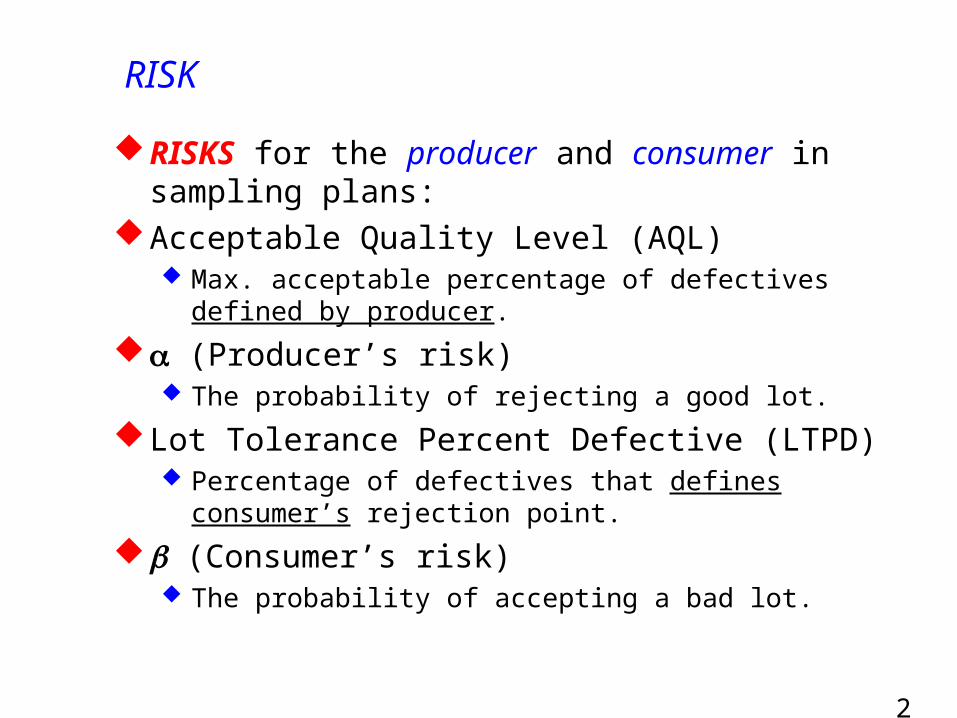
RISKS for the producer and consumer in sampling plans:

Acceptable Quality Level (AQL) Max. acceptable percentage of defectives defined by

producer.

(Producer’s risk) The probability of rejecting a good lot.

Lot Tolerance Percent Defective (LTPD) Percentage of defectives that defines consumer’s

rejection point.

(Consumer’s risk) The probability of accepting a bad lot.

Dr. Saydam, Lecture 1 2

3

9

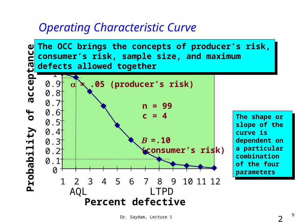
Operating Characteristic Curve

n = 99c = 4

AQL LTPD

00.10.20.30.40.50.60.70.80.9

1

1 2 3 4 5 6 7 8 9 10 11 12

Percent defective

Pro

bab

ilit

y of

acc

epta

nce

=.10(consumer’s risk)

= .05 (producer’s risk)

The OCC brings the concepts of producer’s risk, consumer’s risk, sample size, and maximum defects allowed together

The OCC brings the concepts of producer’s risk, consumer’s risk, sample size, and maximum defects allowed together

The shape or slope of the curve is dependent on a particular combination of the four parameters

The shape or slope of the curve is dependent on a particular combination of the four parameters

Dr. Saydam, Lecture 1 2

4

10

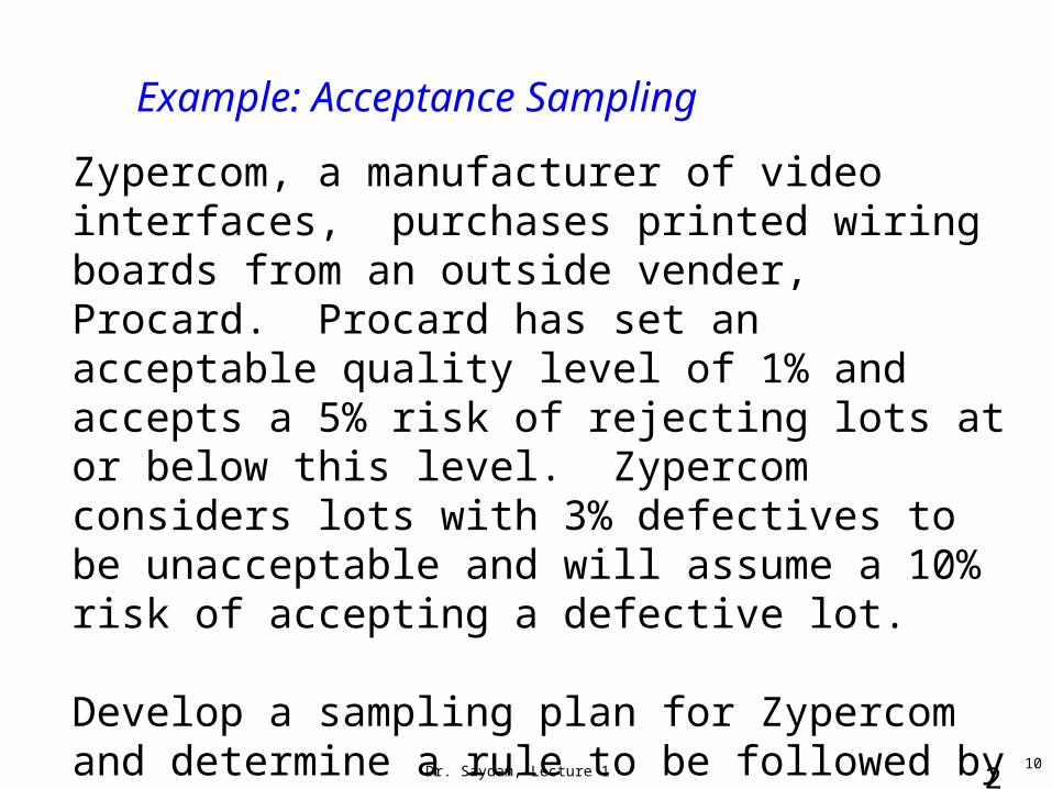
Example: Acceptance Sampling

Zypercom, a manufacturer of video interfaces, purchases printed wiring boards from an outside vender, Procard. Procard has set an acceptable quality level of 1% and accepts a 5% risk of rejecting lots at or below this level. Zypercom considers lots with 3% defectives to be unacceptable and will assume a 10% risk of accepting a defective lot.

Develop a sampling plan for Zypercom and determine a rule to be followed by the receiving inspection personnel.

25

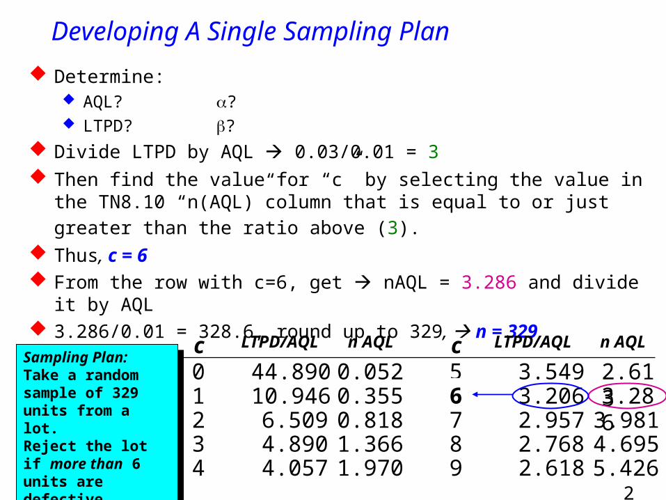
Developing A Single Sampling Plan

Determine: AQL? ? LTPD? ?

Divide LTPD by AQL 0.03/0.01 = 3 Then find the value for “c” by selecting the value in the TN8.10

“n(AQL)”column that is equal to or just greater than the ratio above (3).

Thus, c = 6 From the row with c=6, get nAQL = 3.286 and divide it by

AQL 3.286/0.01 = 328.6, round up to 329, n = 329

c LTPD/AQL n AQL c LTPD/AQL n AQL

0 44.890 0.052 5 3.549 2.6131 10.946 0.355 6 3.206 3.2862 6.509 0.818 7 2.957 3.9813 4.890 1.366 8 2.768 4.6954 4.057 1.970 9 2.618 5.426

Sampling Plan:Take a random sample of 329 units from a lot. Reject the lot if more than 6 units are defective.

Sampling Plan:Take a random sample of 329 units from a lot. Reject the lot if more than 6 units are defective.