sessions 13 & 14 process capability & statistical process control

8/3/2019 Sessions 13 & 14 Process Capability & Statistical Process Control

http://slidepdf.com/reader/full/sessions-13-14-process-capability-statistical-process-control 1/39

1

©The McGraw-Hill Companies, Inc., 2004

Process Capability and Statistical

Quality Control



2


Process Variation

Process Capability

Process Control Procedures

± Variable data

± Attribute data

Acceptance Sampling

± Operating Characteristic Curve

OBJECTIVES



3


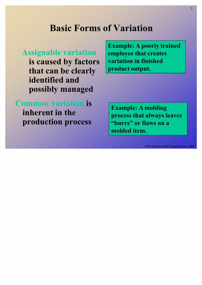
Basic Forms of Variation

Assignable variationis caused by factors

that can be clearlyidentified andpossibly managed

Common variation isinherent in theproduction process

Example: A poorly trained

employee that creates

variation in finished

product output.

Example: A molding

process that always leaves

³burrs´ or flaws on a

molded item.



4


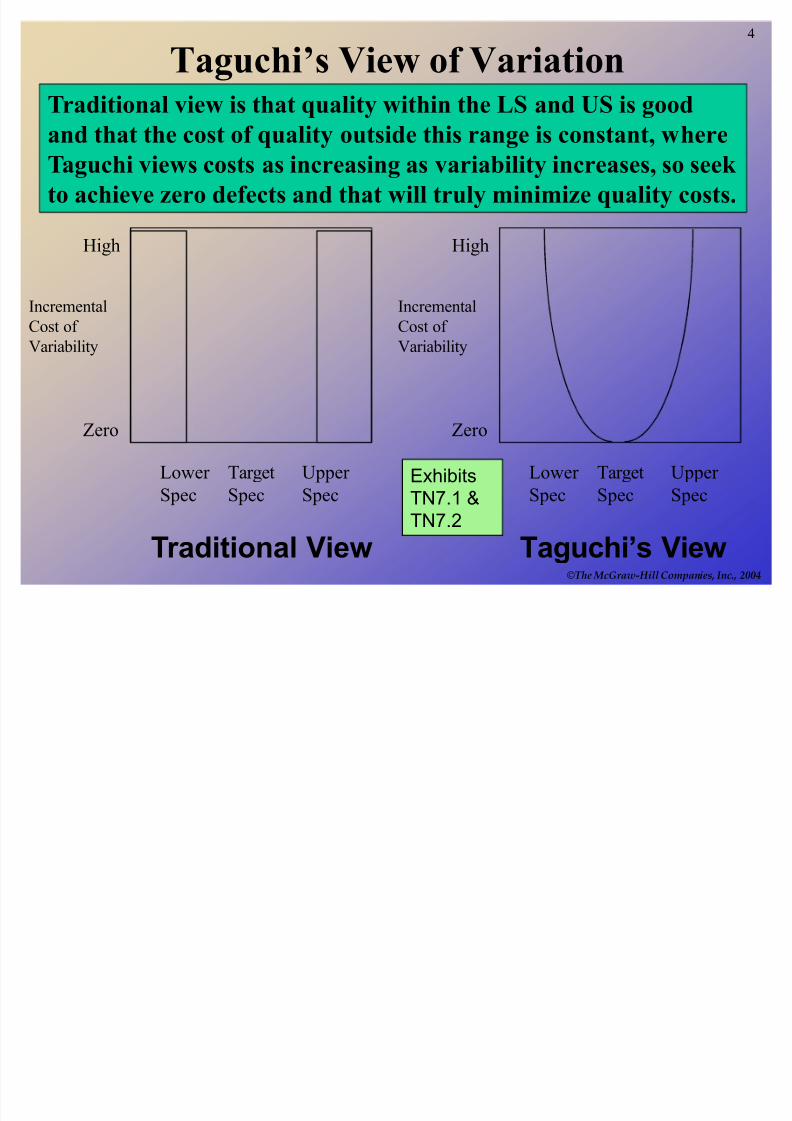
Taguchi¶s View of Variation

Incremental

Cost of

Variability

High

Zero

Lower

Spec

Target

Spec

Upper

Spec

Traditional View

Incremental

Cost of

Variability

High

Zero

Lower

Spec

Target

Spec

Upper

Spec

Taguchi¶s View

Exhibits

TN7.1 &

TN7.2

Traditional view is that quality within the LS and US is good

and that the cost of quality outside this range is constant, whereTaguchi views costs as increasing as variability increases, so seek

to achieve zero defects and that will truly minimize quality costs.



5


Process Capability

Process limits

Tolerance limits

How do the limits relate to one another?



6


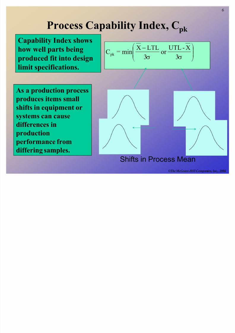
Process Capability Index, Cpk

¹¹ º

¸©©ª

¨

WW 3

X-UTLor

3

LTLXmin=C pk

Shifts in Process Mean

Capability Index showshow well parts being

produced fit into design

limit specifications.

As a production process

produces items small

shifts in equipment or

systems can cause

differences inproduction

performance from

differing samples.



7


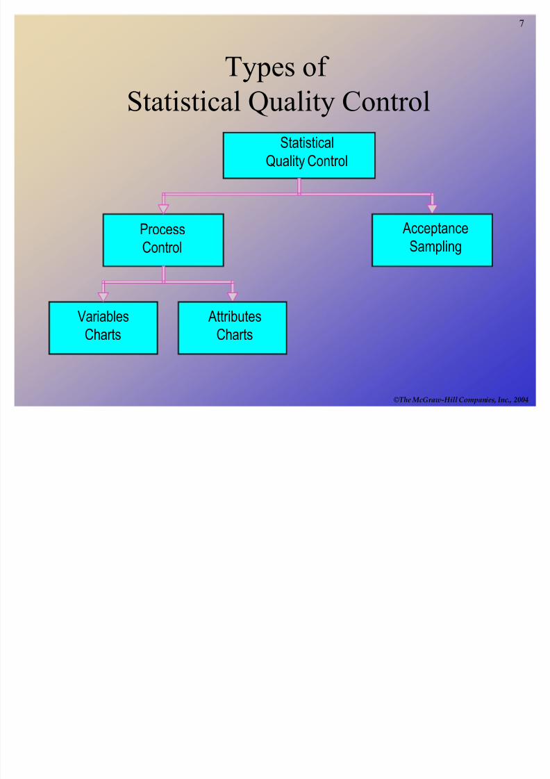
Types of

Statistical Quality ControlStatistical

Quality Control

Process

Control

Acceptance

Sampling

Variables

Charts

Attributes

Charts



8


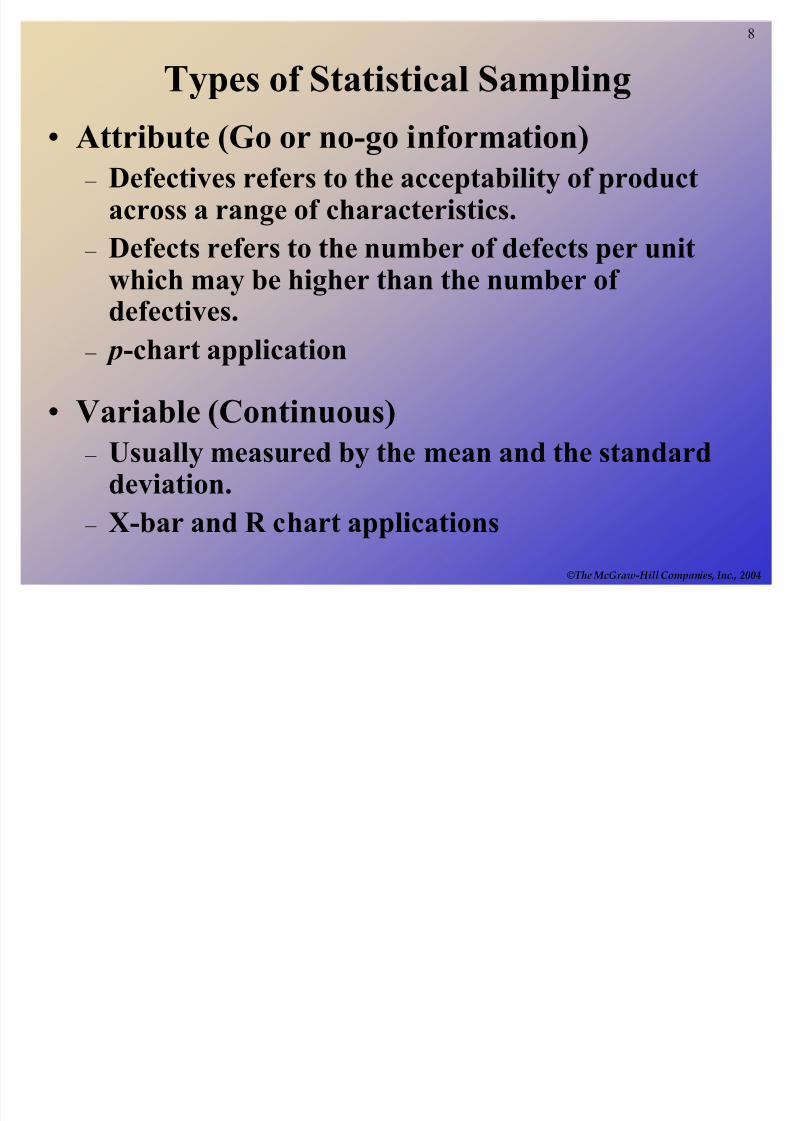
Types of Statistical Sampling

Attribute (Go or no-go information) ± Defectives refers to the acceptability of product

across a range of characteristics.

± Defects refers to the number of defects per unit

which may be higher than the number of defectives.

± p-chart application

Variable (Continuous) ± Usually measured by the mean and the standard

deviation.

± X-bar and R chart applications



9


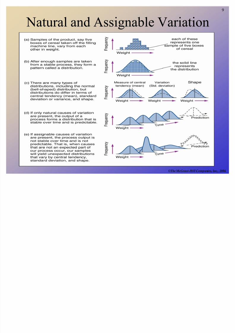
Natural and Assignable Variation



10


UCL

LCL

Samples

over time

1 2 3 4 5 6

UCL

LCL

Samples

over time

1 2 3 4 5 6

UCL

LCL

Samples

over time

1 2 3 4 5 6

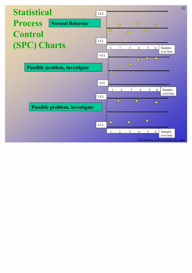
Normal Behavior

Possible problem, investigate

Possible problem, investigate

Statistical

Process

Control(SPC) Charts



11


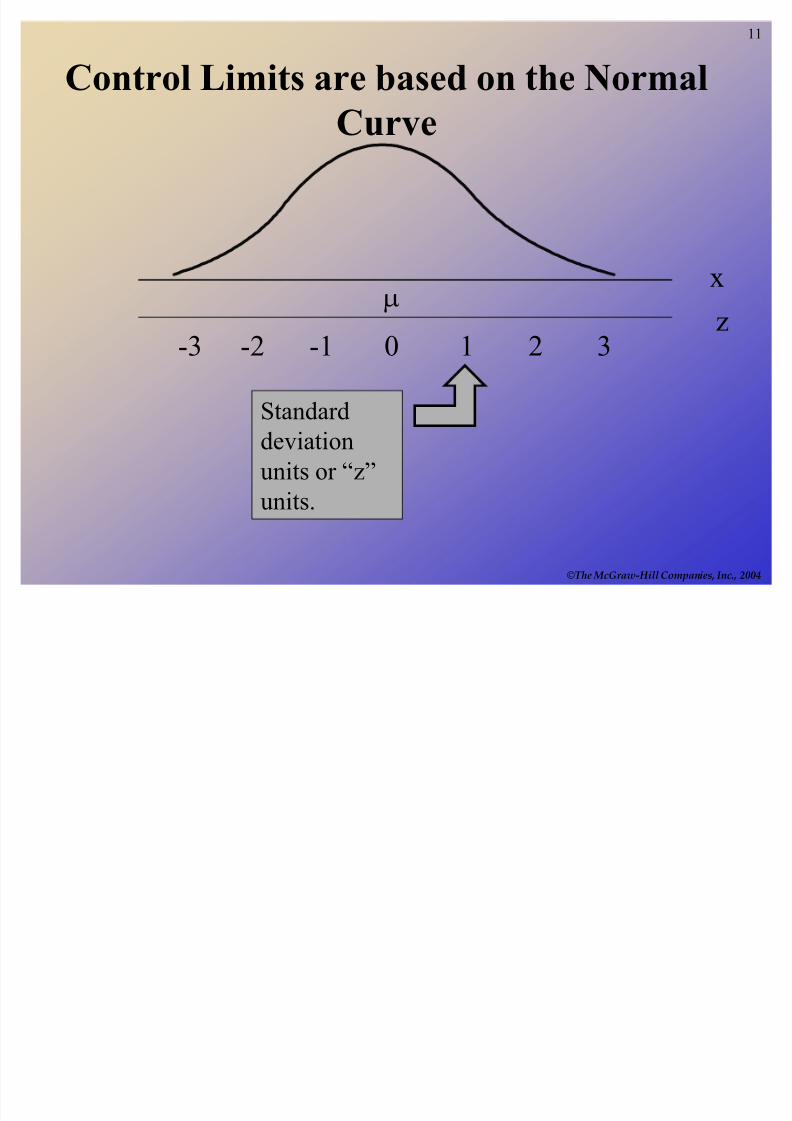
Control Limits are based on the Normal

Curve

x

0 1 2 3-3 -2 -1z

Q

Standarddeviation

units or ³z´

units.



12


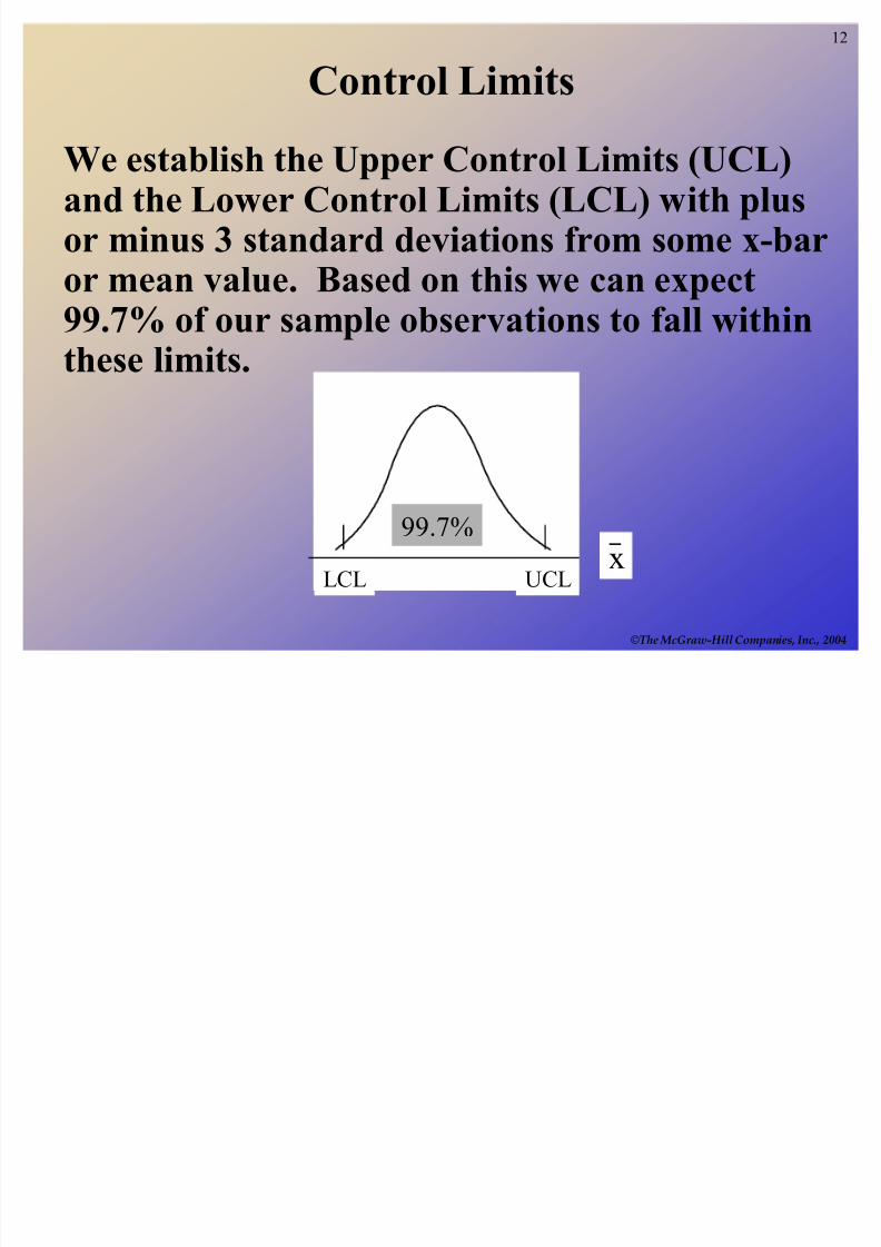
Control Limits

We establish the Upper Control Limits (UCL)and the Lower Control Limits (LCL) with plusor minus 3 standard deviations from some x-baror mean value. Based on this we can expect

99.7% of our sample observations to fall withinthese limits.

xLCL UCL

99.7%



13


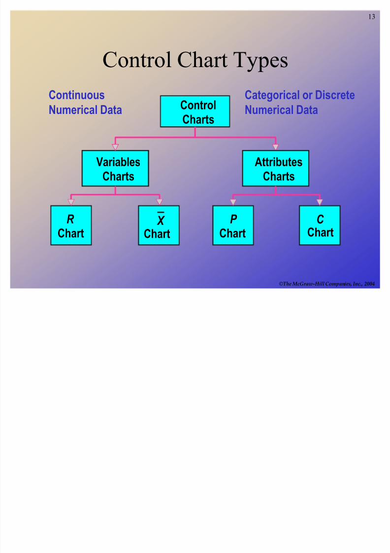
ControlCharts

R

Chart

VariablesCharts

AttributesCharts

X

Chart

P

ChartC

Chart

Continuous

Numerical Data

Categorical or Discrete

Numerical Data

Control Chart Types



14


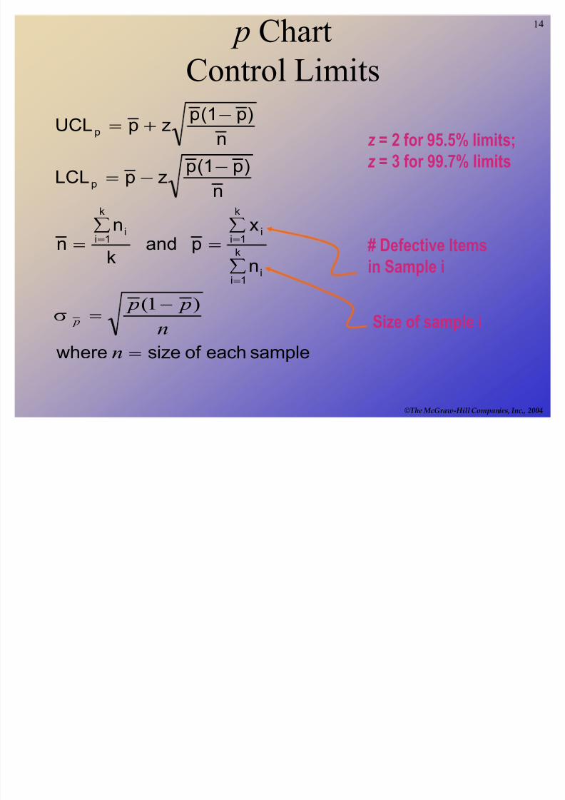
p Chart

Control Limits

# Defective Items

in Sample i

Size of sample i

z = 2 for 95.5% limits;

z = 3 for 99.7% limits

sampleeachof sizewhere

n

xp and

k

nn

n

)p(1pzpLCL

n

)p(1pzpUCL

i

k

1i

i

k

1ii

k

1i

p

p

!

!

§

§

!

§

!

!

!

!

!!

n

n

p p

p

)1( W



15


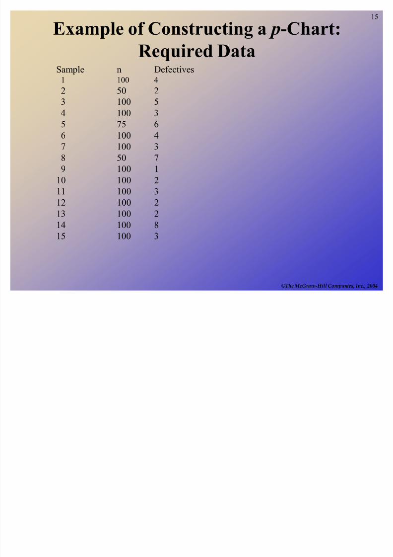
Example of Constructing a p-Chart:

Required DataSample n Defectives

1 100 4

2 50 2

3 100 5

4 100 3

5 75 6

6 100 47 100 3

8 50 7

9 100 1

10 100 2

11 100 3

12 100 213 100 2

14 100 8

15 100 3



16


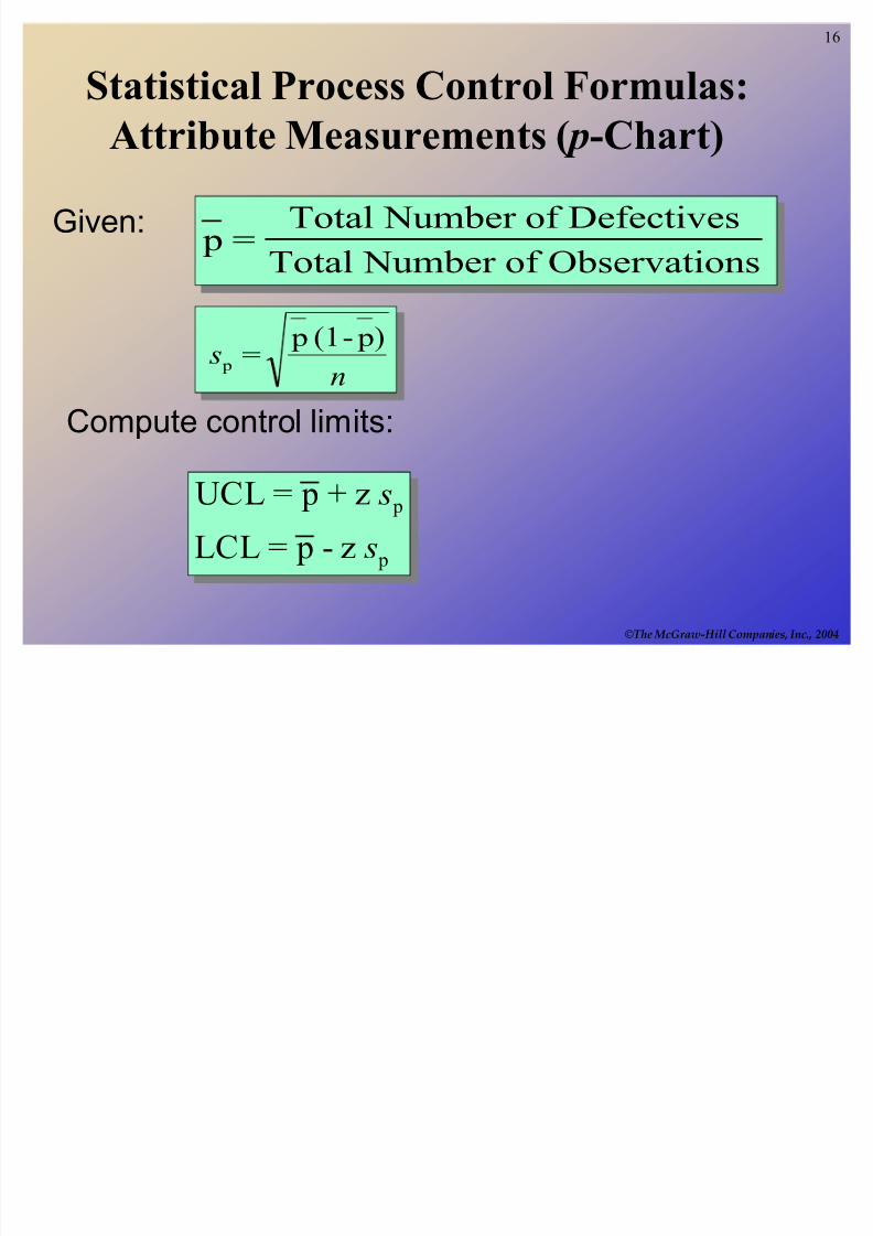
Statistical Process Control Formulas:

Attribute Measurements ( p-Chart)

p =Total Number of Defectives

Total Number of Observations

n

s

) p-(1 p = p

p

p

z- p=LCL

z+ p=UCL

s

s

Given:

Compute control limits:



17


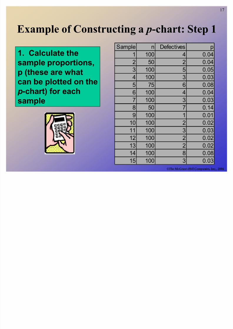
1. Calculate the

sample proportions,

p (these are what

can be plotted on the p-chart) for each

sample

Sample n Defectives p

1 100 4 0.04

2 50 2 0.04

3 100 5 0.05

4 100 3 0.03

5 75 6 0.08

6 100 4 0.04

7 100 3 0.03

8 50 7 0.14

9 100 1 0.01

10 100 2 0.0211 100 3 0.03

12 100 2 0.02

13 100 2 0.02

14 100 8 0.08

15 100 3 0.03

Example of Constructing a p-chart: Step 1



18


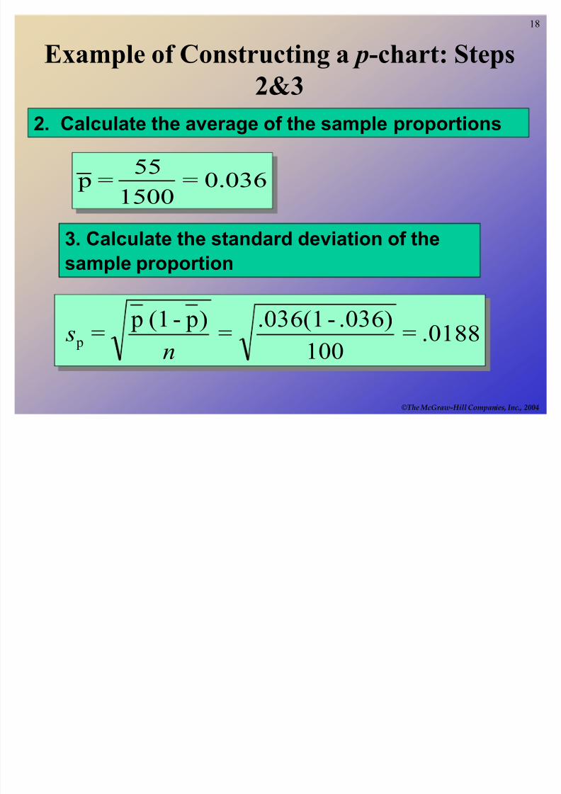
2. Calculate the average of the sample proportions

0.036=

1500

55 = p

3. Calculate the standard deviation of the

sample proportion

.0188=100

.036)-.036(1=

) p-(1 p = p

n

s

Example of Constructing a p-chart: Steps

2&3



19


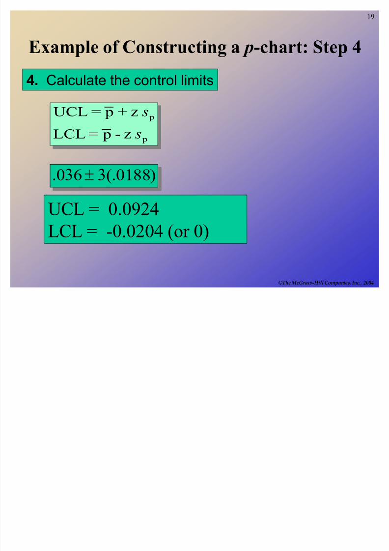
4. Calculate the control limits

3(.0188).036s

UCL = 0.0924LCL = -0.0204 (or 0)

p

p

z- p=LCL

z+ p=UCL

s

s

Example of Constructing a p-chart: Step 4



20


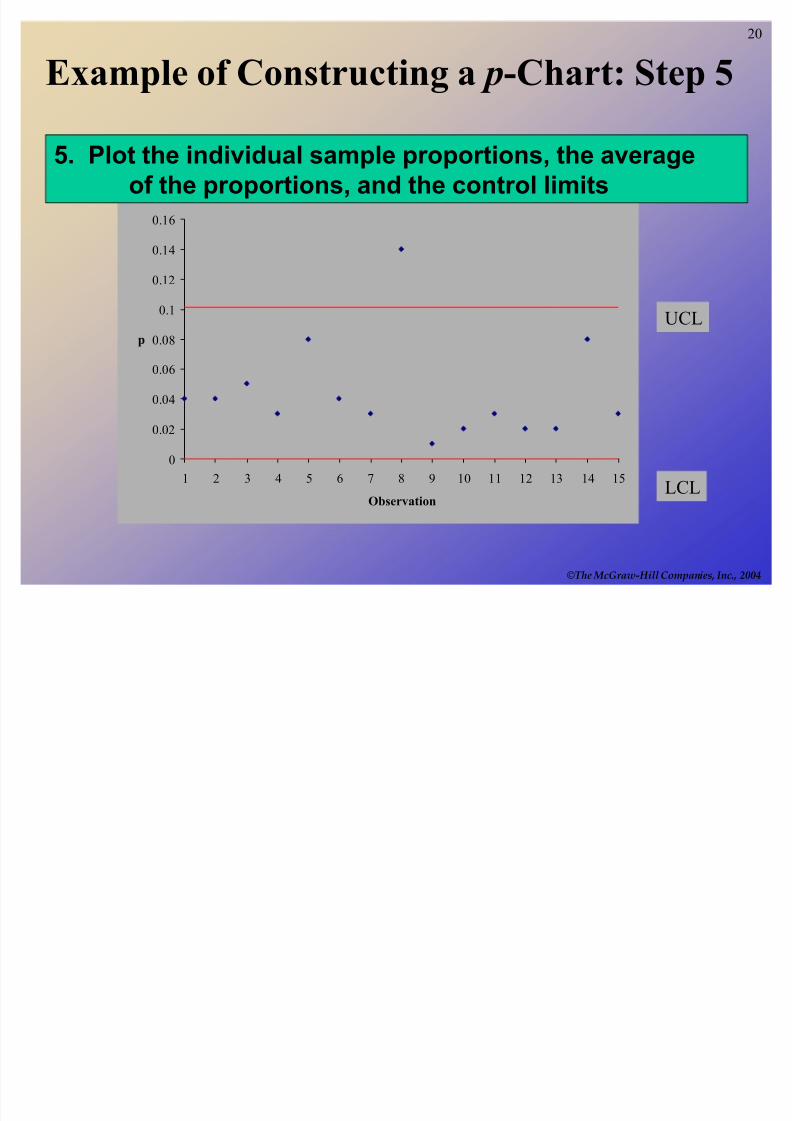
Example of Constructing a p-Chart: Step 5

0

0.02

0.04

0.06

0.08

0.1

0.12

0.14

0.16

1 2 3 4 5 6 7 8 9 10 11 12 13 14 15

Observation

p

UCL

LCL

5. Plot the individual sample proportions, the average

of the proportions, and the control limits



21


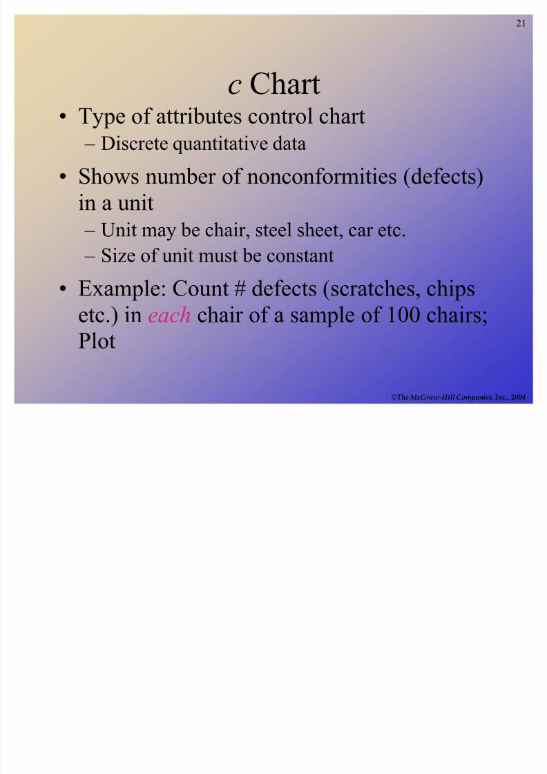
Type of attributes control chart

± Discrete quantitative data

Shows number of nonconformities (defects)

in a unit

± Unit may be chair, steel sheet, car etc.

± Size of unit must be constant

Example: Count # defects (scratches, chipsetc.) in each chair of a sample of 100 chairs;Plot

cChart



22


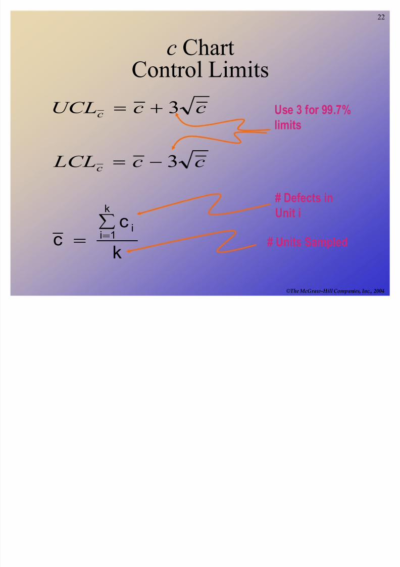
c Chart

Control Limits

# Defects in

Unit i

# Units Sampled

Use 3 for 99.7%

limits

k

c c

i

k

1i!§

!

!

!

cc LCL

ccUCL

c

c

3

3



23


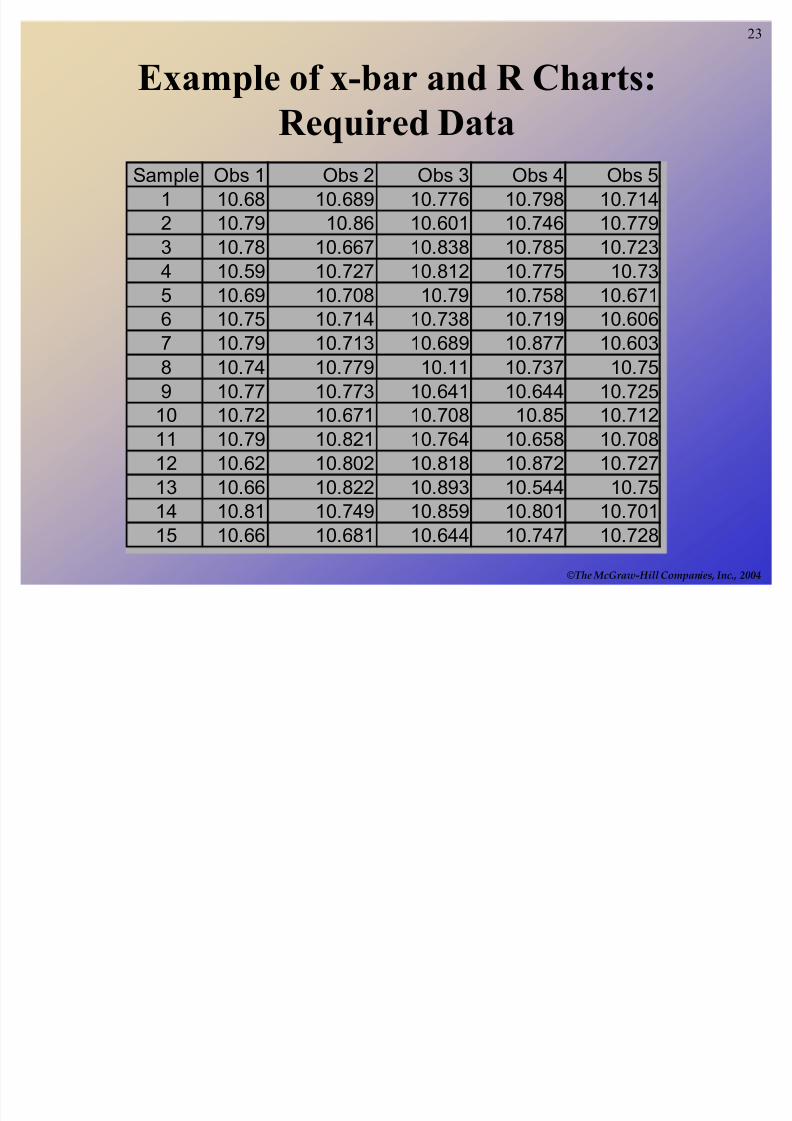
Example of x-bar and R Charts:

Required DataSample Obs 1 Obs 2 Obs 3 Obs 4 Obs 5

1 10.68 10.689 10.776 10.798 10.714

2 10.79 10.86 10.601 10.746 10.779

3 10.78 10.667 10.838 10.785 10.723

4 10.59 10.727 10.812 10.775 10.735 10.69 10.708 10.79 10.758 10.671

6 10.75 10.714 10.738 10.719 10.606

7 10.79 10.713 10.689 10.877 10.603

8 10.74 10.779 10.11 10.737 10.75

9 10.77 10.773 10.641 10.644 10.725

10 10.72 10.671 10.708 10.85 10.71211 10.79 10.821 10.764 10.658 10.708

12 10.62 10.802 10.818 10.872 10.727

13 10.66 10.822 10.893 10.544 10.75

14 10.81 10.749 10.859 10.801 10.701

15 10.66 10.681 10.644 10.747 10.728



24


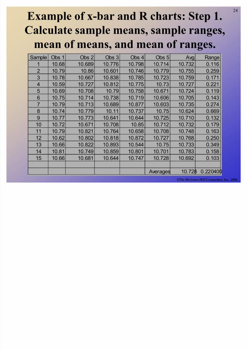
Example of x-bar and R charts: Step 1.

Calculate sample means, sample ranges,

mean of means, and mean of ranges.Sample Obs 1 Obs 2 Obs 3 Obs 4 Obs 5 Avg Range

1 10.68 10.689 10.776 10.798 10.714 10.732 0.116

2 10.79 10.86 10.601 10.746 10.779 10.755 0.259

3 10.78 10.667 10.838 10.785 10.723 10.759 0.171

4 10.59 10.727 10.812 10.775 10.73 10.727 0.221

5 10.69 10.708 10.79 10.758 10.671 10.724 0.119

6 10.75 10.714 10.738 10.719 10.606 10.705 0.143

7 10.79 10.713 10.689 10.877 10.603 10.735 0.274

8 10.74 10.779 10.11 10.737 10.75 10.624 0.669

9 10.77 10.773 10.641 10.644 10.725 10.710 0.132

10 10.72 10.671 10.708 10.85 10.712 10.732 0.179

11 10.79 10.821 10.764 10.658 10.708 10.748 0.16312 10.62 10.802 10.818 10.872 10.727 10.768 0.250

13 10.66 10.822 10.893 10.544 10.75 10.733 0.349

14 10.81 10.749 10.859 10.801 10.701 10.783 0.158

15 10.66 10.681 10.644 10.747 10.728 10.692 0.103

Averages 10.728 0.220400



25


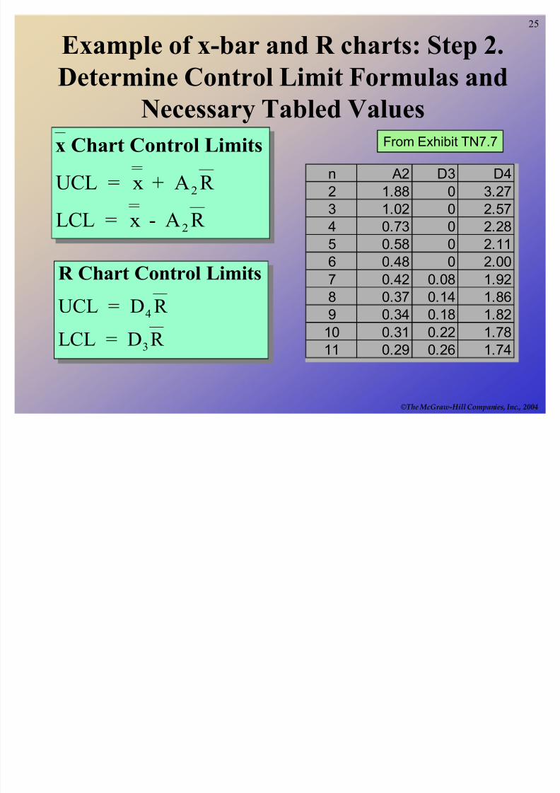
Example of x-bar and R charts: Step 2.

Determine Control Limit Formulas and

Necessary Tabled Values

x Chart Control Limits

UCL = x + A R

LCL = x - A R

2

2

R Chart Control Limits

UCL = D R

LCL = D R

4

3

From Exhibit TN7.7

n A2 D3 D4

2 1.88 0 3.273 1.02 0 2.57

4 0.73 0 2.28

5 0.58 0 2.11

6 0.48 0 2.00

7 0.42 0.08 1.92

8 0.37 0.14 1.869 0.34 0.18 1.82

10 0.31 0.22 1.78

11 0.29 0.26 1.74



26


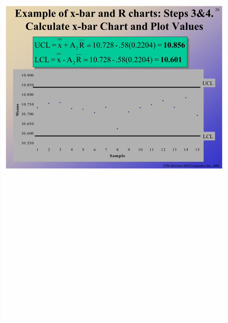
Example of x-bar and R charts: Steps 3&4.

Calculate x-bar Chart and Plot Values

10.601

10.856

=).58(0.2204-10.728R A-x=LCL

=).58(0.2204-10.728R A+x=UCL

2

2

!

!

10 .55 0

10 .600

10 .65 0

10 .700

10.75 0

10.800

10.85 0

10.900

1 2 3 4 5 6 7 8 9 10 11 12 13 14 15

Sample

M e a n s

UCL

LCL



27


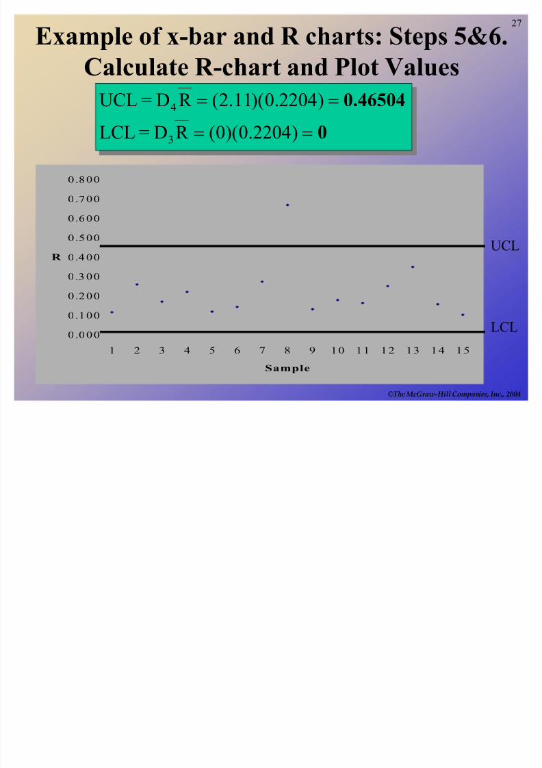
Example of x-bar and R charts: Steps 5&6.

Calculate R-chart and Plot Values

0

0.46504

!!

!!

)2204.0)(0(R D=LCL

)2204.0)(11.2(R D=UCL

3

4

0 .0 0 0

0 .1 0 0

0 .2 0 0

0 .30 0

0 .40 0

0 .5 0 0

0 .6 0 0

0 .7 0 0

0 .8 0 0

1 2 3 4 5 6 7 8 9 1 0 1 1 1 2 13 14 1 5

Sample

R UCL

LCL



28


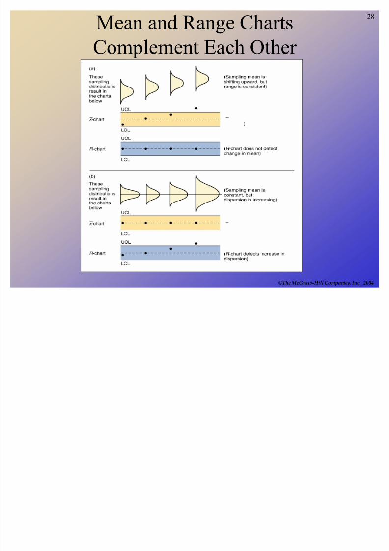
Mean and Range Charts

Complement Each Other



29


Basic Forms of Statistical Sampling for

Quality Control

Acceptance Sampling is sampling to

accept or reject the immediate lot of product at hand

Statistical Process Control is sampling to

determine if the process is within

acceptable limits



30


Acceptance Sampling Purposes

± Determine quality level

± Ensure quality is within predetermined level

Advantages

± Economy ± Less handling damage

± Fewer inspectors

± Upgrading of the inspection job

± Applicability to destructive testing

± Entire lot rejection (motivation for improvement)



31


Acceptance Sampling (Continued)

Disadvantages

± Risks of accepting ³bad´ lots and rejecting

³good´ lots

± Added planning and documentation

± Sample provides less information than 100-

percent inspection



32


Acceptance Sampling:

Single Sampling Plan

A simple goal

Determine (1) how many units, n,to sample from a lot, and (2) themaximum number of defective

items, c, that can be found in thesample before the lot is rejected



33


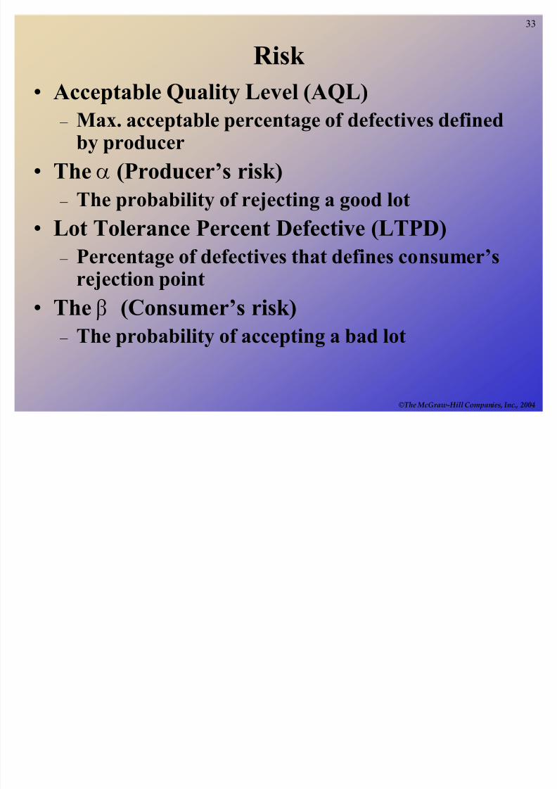
Risk

Acceptable Quality Level (AQL) ± Max. acceptable percentage of defectives defined

by producer

The E(Producer¶s risk)

± The probability of rejecting a good lot

Lot Tolerance Percent Defective (LTPD)

± Percentage of defectives that defines consumer¶srejection point

The F (Consumer¶s risk)

± The probability of accepting a bad lot



34


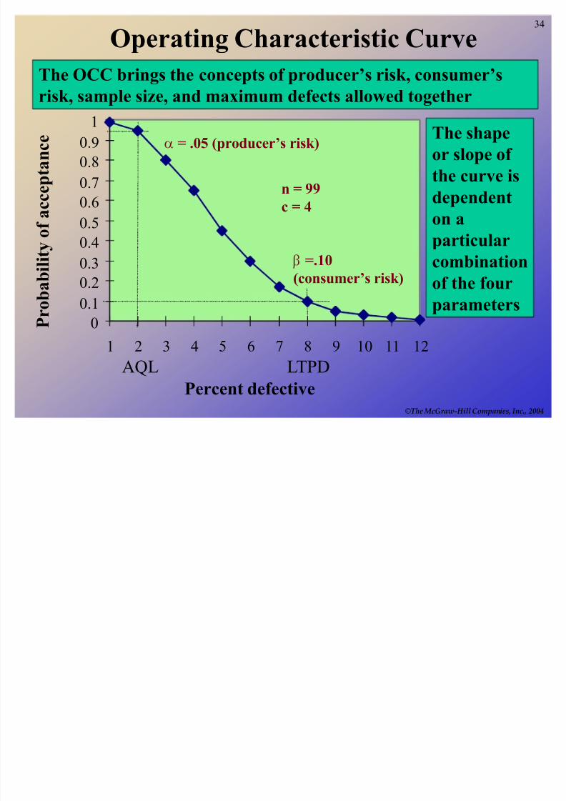
Operating Characteristic Curve

n = 99

c = 4

AQL LTPD

00.1

0.2

0.3

0.4

0.5

0.6

0.7

0.8

0.9

1

1 2 3 4 5 6 7 8 9 10 11 12

Percent defective

P r o b

a b i l i t y o f a c c

e p t a n c e

F =.10

(consumer¶s risk)

E= .05 (producer¶s risk)

The OCC brings the concepts of producer¶s risk, consumer¶s

risk, sample size, and maximum defects allowed together

The shape

or slope of

the curve is

dependenton a

particular

combination

of the four

parameters



35


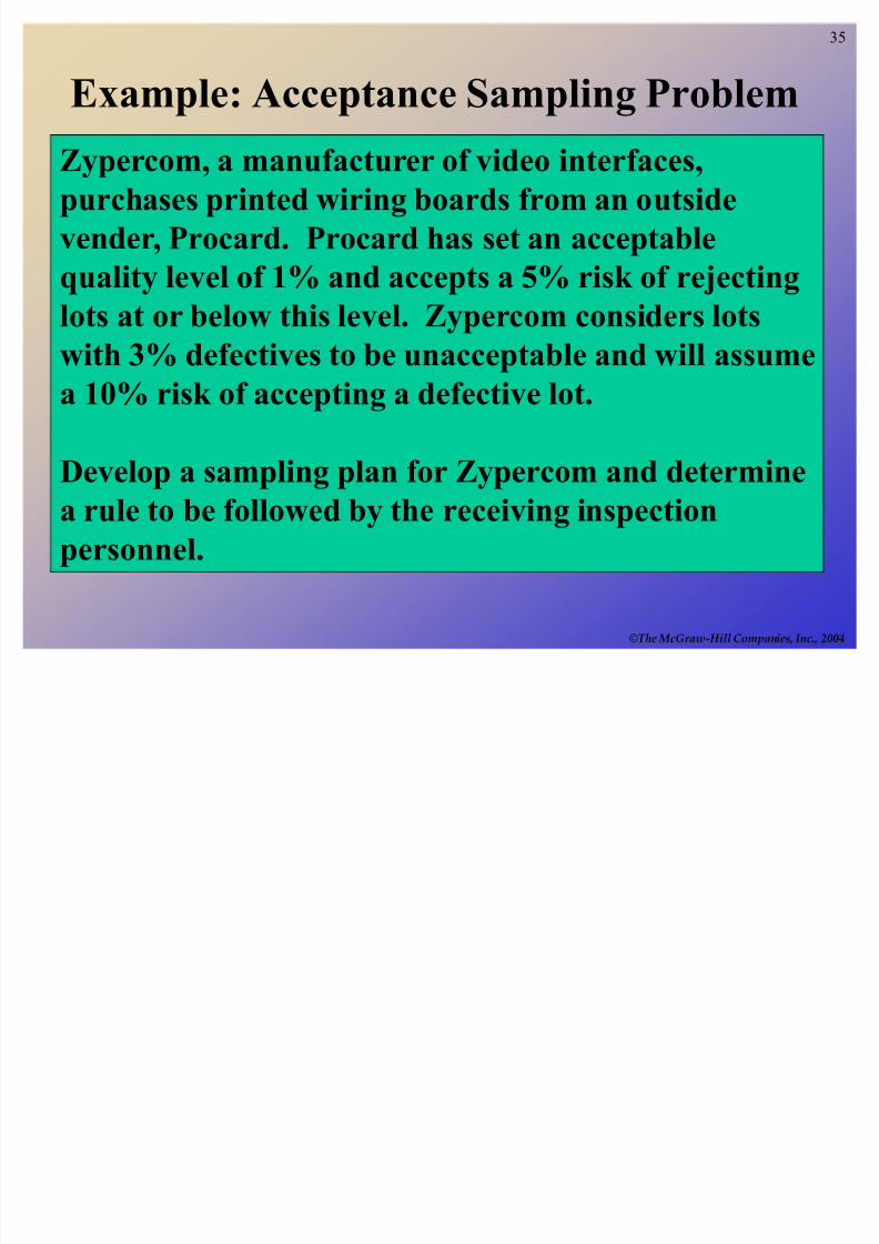
Example: Acceptance Sampling Problem

Zypercom, a manufacturer of video interfaces,purchases printed wiring boards from an outside

vender, Procard. Procard has set an acceptable

quality level of 1% and accepts a 5% risk of rejecting

lots at or below this level. Zypercom considers lotswith 3% defectives to be unacceptable and will assume

a 10% risk of accepting a defective lot.

Develop a sampling plan for Zypercom and determinea rule to be followed by the receiving inspection

personnel.



36


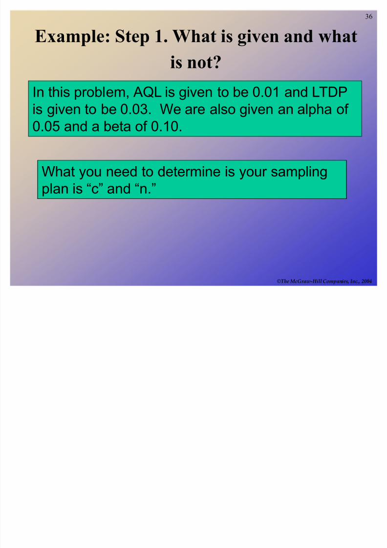
Example: Step 1. What is given and what

is not? In this problem, AQL is given to be 0.01 and LTDP

is given to be 0.03. We are also given an alpha of

0.05 and a beta of 0.10.

What you need to determine is your sampling

plan is ³c´ and ³n.´



37


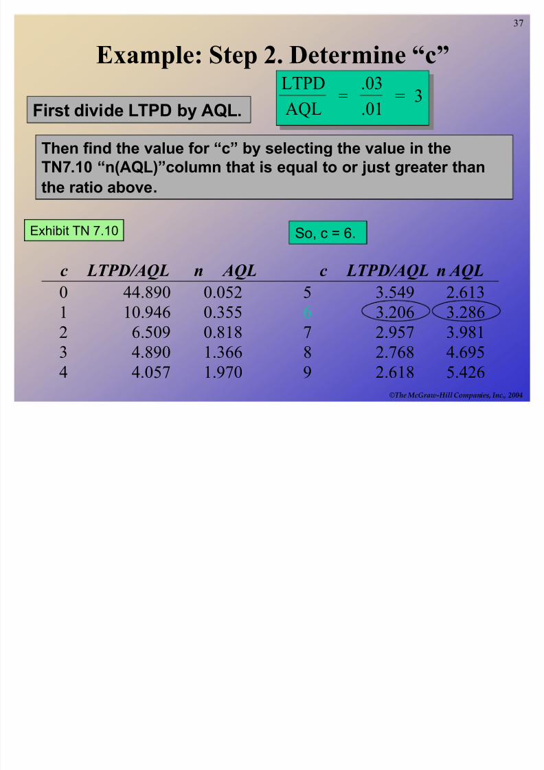
Example: Step 2. Determine ³c´

First divide LTPD by AQL.

LTPD

AQL =

.03

.01 = 3

Then find the value for ³c´ by selecting the value in the

TN7.10 ³n(AQL)´column that is equal to or just greater than

the ratio above.

Exhibit TN 7.10

c LTPD/AQL n AQL c LTPD/AQL n AQL

0 44.890 0.052 5 3.549 2.6131 10.946 0.355 6 3.206 3.286

2 6.509 0.818 7 2.957 3.981

3 4.890 1.366 8 2.768 4.695

4 4.057 1.970 9 2.618 5.426

So, c = 6.



38


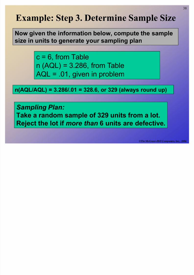
Example: Step 3. Determine Sample Size

c = 6, from Table

n (AQL) = 3.286, from Table AQL = .01, given in problem

Sampling Plan:

Take a random sample of 329 units from a lot.

Reject the lot if more than 6 units are defective.

Now given the information below, compute the samplesize in units to generate your sampling plan

n(AQL/AQL) = 3.286/.01 = 328.6, or 329 (always round up)



39


End of SPC

sessions 13 & 14 process capability & statistical process control

Documents