allocation of two dimensional parts using a shape

Louisiana State UniversityLSU Digital Commons

LSU Historical Dissertations and Theses Graduate School

1996

Allocation of Two Dimensional Parts Using aShape Reasoning Heuristic.Henry Joseph Lamousin IIILouisiana State University and Agricultural & Mechanical College

Follow this and additional works at: https://digitalcommons.lsu.edu/gradschool_disstheses

This Dissertation is brought to you for free and open access by the Graduate School at LSU Digital Commons. It has been accepted for inclusion inLSU Historical Dissertations and Theses by an authorized administrator of LSU Digital Commons. For more information, please [email protected].

Recommended CitationLamousin, Henry Joseph III, "Allocation of Two Dimensional Parts Using a Shape Reasoning Heuristic." (1996). LSU HistoricalDissertations and Theses. 6351.https://digitalcommons.lsu.edu/gradschool_disstheses/6351

https://digitalcommons.lsu.edu?utm_source=digitalcommons.lsu.edu%2Fgradschool_disstheses%2F6351&utm_medium=PDF&utm_campaign=PDFCoverPages

https://digitalcommons.lsu.edu/gradschool_disstheses?utm_source=digitalcommons.lsu.edu%2Fgradschool_disstheses%2F6351&utm_medium=PDF&utm_campaign=PDFCoverPages

https://digitalcommons.lsu.edu/gradschool?utm_source=digitalcommons.lsu.edu%2Fgradschool_disstheses%2F6351&utm_medium=PDF&utm_campaign=PDFCoverPages

https://digitalcommons.lsu.edu/gradschool_disstheses?utm_source=digitalcommons.lsu.edu%2Fgradschool_disstheses%2F6351&utm_medium=PDF&utm_campaign=PDFCoverPages

https://digitalcommons.lsu.edu/gradschool_disstheses/6351?utm_source=digitalcommons.lsu.edu%2Fgradschool_disstheses%2F6351&utm_medium=PDF&utm_campaign=PDFCoverPages

mailto:[email protected]

INFORMATION TO USERS

This manuscript has been reproduced from the microfilm master. UME

films the text directly from the original or copy submitted. Thus, some

thesis and dissertation copies are in typewriter free, while others may be

from any type of computer printer.

The quality of this reproduction is dependent upon the quality of the

copy submitted. Broken or indistinct print, colored or poor quality

illustrations and photographs, print bleedthrough, substandard margins,

and improper alignment can adversely afreet reproduction.

In the unlikely event that the author did not send UMI a complete

manuscript and there are missing pages, these will be noted. Also, if

unauthorized copyright material had to be removed, a note will indicate

the deletion.

Oversize materials (e.g., maps, drawings, charts) are reproduced by

sectioning the original, beginning at the upper left-hand comer and

continuing from left to right in equal sections with small overlaps. Each

original is also photographed in one exposure and is included in reduced

form at the back of the book.

Photographs included in the original manuscript have been reproduced

xerographically in this copy. Higher quality 6” x 9” black and white

photographic prints are available for any photographs or illustrations

appearing in this copy for an additional charge. Contact UMI directly to

order.

UMIA Bell & Howell Infoimaticn Company

300 North Zeeb Road, Ann Arbor MI 48106-1346 USA 313/761-4700 800/521-0600

Reproduced with permission of the copyright owner. Further reproduction prohibited without permission.

ALLOCATION OF TWO DIMENSIONAL PARTS USING A

SHAPE REASONING HEURISTIC

A Dissertation

Submitted to the Graduate Faculty of the Louisiana State University and

Agricultural and Mechanical College in partial fulfillment of the

requirements for the degree of Doctor of Philosophy

m

The Department of Mechanical Engineering

byHenry J. Lamousin III

B.S., University of New Orleans, 1987 December 1996


UMI Number: 9720365

UMI Microform 9720365 Copyright 1997, by UMI Company. All rights reserved.

This microform edition is protected against unauthorized copying under Title 17, United States Code.

UMI300 North Zeeb Road Ann Arbor, MI 48103


A cknow ledgm entsFirst and foremost I would like to thank my mother,

Rosemary, for her patronage and patience throughout what by all meas

ures has been a lengthy graduate career. Without her generous support

much of the work accomphshed would not be have been possible. I would

also like to acknowledge Mr. Jules Hubert for the companionship and

wise council he has offered my mother throughout my studies. His friend

ship has proven invaluable in achieving my goals.

I would like to express appreciation to the professors serving

on my committee for their time and efforts. These are Doctors Sumanta

Acharya, T. Warren Liao, Michael Murphy, Dirk Smith, Neal Stoltzfus,

and Warren Waggenspack. In particular I would like to thank Doctors

Smith and Murphy for the many helpful suggestions they have made in

editing this manuscript. I am also grateful to Dr. Waggenspack for his

service as my major professor, and for the liberties and professional cour

tesies granted me in conducting this research.

I would like to thank McDermott Inc. for the stimulus and

original funding behind this work, and recognize the efforts of Mr. Mark

Adams in contributing the data sets used for evaluation. This work was

also supported in part by a fellowship from the Board of Regents.

A pledge of gratitude is accorded the many individuals who

have tolerated my pranks, extreme moods, and endless diatribes over the

years. My fellow lab mates have taken the brunt of this burden, includ

ing: Robert Benton, Sandeep Danni, Siddarameshwar Bagah, Yohannes

Desta, Olalekan Odesanya, David Thompson, Ramji Venkatachari and

Tarek Zohdi. I would also like to express my gratefulness to Aleric Haag

u


for his endeavors in maintaining the computer facilities of the Interactive

Modeling Research Laboratory, where the majority of this work was com

pleted. To aU of you and numerous others, thanks.

Finally, I would like to convey my deepest appreciation to

two special individuals, Laura Gough and Gregory Dobson. Laura has

shared in the emotional highs and lows, provided a much needed calming

voice on many occasions, and proved an indispensable companion over

these last two trying years. The value of Greg’s service as a sounding

board for the numerous solutions to my assorted technical and personal

problems cannot be calculated. I owe my success and sanity in great part

to his good advice and unwavering friendship over the years. T han k s!

m


Table o f C ontentsA c k n o w le d g e m e n t s ............................................................................. iiL i s t o f T a b l e s ..........................................................................................viiL i s t o f F i g u r e s ...................................................................................... viiiA b s t r a c t ..................................................................................................xiiiC h a p te r 1I n t r o d u c t i o n a n d L i t e r a t u r e R e v ie w ....................................... 1

1.1 The Allocation Problem in In d u stry .............................................. 11.2 Classification of Allocation Problems ............................................ 31.3 The Problem Investigated...............................................................71.4 Classification of Solution Techniques ........................................... 8

1.4.1 Rectangular Approximation Placement S trategies 101.4.2 Optimization Methods ........................................................11

1.4.2.1 The Objective or Cost Function ......................... 131.4.2.2 Simulated Annealing Techniques ...................... 151.4.2.3 Genetic Algorithms ..............................................17

1.4.3 Rule Based, Intelligent, & Expert Systems ......................201.4.3.1 Fixed Orientation Boundary

Abutting Techniques .......................................... 201.4.3.2 Shape Based Techniques ....................................22

1.5 Dissertation Layout ......................................................................29C h a p te r 2T h e P i lo t S tu d y ....................................................................................30

2.1 Introduction and Background...................................................... 302.2 The Method of Albano and Sapuppo ...........................................31

2.2.1 Part Placement ...................................................................312.2.2 Part Selection ......................................................................41

2.3 Adaptations ................................................................................... 442.3.1 Irregular Resources .............................................................442.3.2 Part Simplification..............................................................502.3.3 Optimal Part O rientation...................................................52

2.4 Pilot Study Sum m ary....................................................................57

IV


Chapter 3 Shape R easoningand the Feature Based Approach ............................................60

3.1 Introduction ...................................................................................603.2 Features .........................................................................................603.3 Profile Simplification Techniques ............................................... 64

3.3.1 Small Complexity Reduction .............................................653.3.2 Large Scale Resource Division ..........................................70

3.4 Void Simplification........................................................................ 753.5 Part Simplification .........................................................................763.6 Feature Extraction and Storage ................................................... 77

Chapter 4N esting w ith F ea tu res .................................................................... 81

4.1 Introduction ...................................................................................814.2 Part Placement ............................................................................. 81

4.2.1 Orientation ......................................................................... 824.2.2 Align Types ........................................................................ 844.2.3 Initial Placement and Shifting..........................................90

4.3 Part Selection ............................................................................... 94Chapter 5Im plem entation and Results .....................................................100

5.1 Introduction .................................................................................1005.2 Search Algorithm ....................................................................... 1005.3 Waste Function .......................................................................... 1035.4 Matching Index Tolerances........................................................ 1075.5 Results ........................................................................................108

5.5.1 Parameter S tudy .............................................................. I l l5.5.2 Analysis of All Cases ....................................................... 121

Chapter 6C onclusions and Future W ork ................................................. 125

6.1 Summary .....................................................................................1256.2 Shape Reasoning Advantages and Limitations ....................... 1266.3 Future Work ............................................................................... 128


Bibliography ...................................................................................... 132Appendix .............................................................................................. 140

A.1 Align Types ................................................................................... 140A.2 A Sample Problem Description................................................... 148A 3 Feature Based Solution Layouts ................................................ 153A.4 NFP Based Solution Layouts...................................................... 168

V ita ..........................................................................................................183

VI


L ist o f T ables5.1 Matching Index Tolerance Values................................................. 108

5.2 Problem set overall characteristics............................................... 112

5.3 Summary of results with border restrictions set to 180“—>360°.Asterisks denote feature based solutions requiring fewer plates than the NFP technique.....................................................113

5.4 Summary of results with border restrictions alternating between 90“->180“ and 180“->270“. Asterisks denote feature based solutions requiring fewer plates than theNFP technique............................................................................... 114

5.5 Summary of CPU time per part reslut for the parameterstudy...............................................................................................115

5.6 Individual plate results for problem set C (Figure 5.5).N_SUCCESSOR equals 20........................................................... 116

5.7 Individual plate results for problem set H (Figure 5.6).N_SUCCESSOR equals 20........................................................... 116

5.8 Results for all cases. N_SUCCESSOR equals 20. Borderrestrictions alternate between 90“->180“ and 180°—>270“........122

A. 1.1 Align Types for Side One Alignment........................................... 141

A. 1.2 Align Types for Side Two Alignment........................................... 143

A. 1.3 Align Types for Side Three Alignment........................................ 146

vu


L ist o f F igures1.1 Three examples demonstrating the one, two and three

dimension aspects of the allocation problem..................................2

1.2 Different layout or pattern types: (a) guillotine, (b) nonguillotine or nested, (c) non-orthogonal...........................................6

1.3 Rectangular Approximation Methods............................................ 12

1.4 Flow diagram showing the basic steps of simulatedannealing..........................................................................................16

1.5 Operators used in the genetic algorithm: (a) Crossover,(b) M utation .................................................................................... 19

1.6 The method of Dagli and Totoglu. Part placements are generated by pairwise matches of all sides of parts A and B.The location producing the smallest MER is selected as best... 23

1.7 Cheok and Nee's rule based methods. Parts are classifiedinto groups and packed into rectangular modules....................... 25

1.8 Several orientation invariant measures of shape or "chainlet features" used by Haims to solve the apictorial jigsaw puzzle problem. Chainlets are formed by dividing profiles atcritical points................................................................................... 26

1.9 Chung's method. Profiles are placed using the outer anglesof the "abstract polygon" representing each part......................... 28

2.1 Generating a No Fit Polygon (NFP)...............................................32

2.2 Initial positioning to generate the NFP between Parts Aand B showing the direction of movement and contact vertices..............................................................................................35

2.3 Determining the extent of movement a t each stage as part Bmoves around part A in a counterclockwise direction................. 36

2.4 A group of parts and their associated Merged Profile..................37

2.5 Savings through elimination of edges and vertices duringNFP intersection calculations....................................................... 39

2.6 Part placement withing the allocation region.............................. 40

2.7 A complete allocation tree for 4 parts with only oneorientation allowed..........................................................................41

vu i


2.8 A trimmed allocation tree showing the optimum search path .. 42

2.9 The true waste associated with a layout.......................................43

2.10 The method of Albano and Sapuppo applied directly to irregular resources. Note that the allocation region is the area enclosed by the NFP of B on the interior boundary ofthe resource..................................................................................... 45

2.11 Part placement in voids using the Internal No Fit Polygon 47

2.12 Generating Initial Placements through convex decompositon.. 49

2.13 The modified convex hull part simplification procedureshowing the total incorporation of concave regions.................... 51

2.14 The modified convex hull part simplification procedureshowing simplification of a concave region.................................. 53

2.15 The primary orientation for nesting within voids........................ 54

2.16 Four orientations produce the same leftmost lowest placment. Orientation priorities are used to select the best placement 55

2.17 Above and left area calculation technique..................................... 56

2.18 Drawbacks of standard orientations and a placement policy.... 58

3.1 Two and three sided features as consecutive edges on partand void (remaining resource) profiles. Part features are convex, while voids are concave.....................................................62

3.2 The utility of shape characteristics at various levels of detailduring part placement.................................................................... 63

3.3 A convex ridge and concave shallow and their associatedheights.............................................................................................66

3.4 Convex shallow elimination m ethods............................................66

3.5 Convex ridge simplification showing the two possible caseswith the trailing edge......................................................................68

3.6 Edge heights and chamfer elimination.........................................69

3.7 The LSRD process. Quadruples preceding each action represent values of the decision criteria (Area, Concave, Side, MER) for that subregion. Asterisks indicate the criteria isnot required to determine the action shown.................................71

IX


3.8 Decision tree showing the action taken for void subregioncriteria ............................................................................................. 72

3.9 Differtent levels of detail produced by varying the area anddivision tolerances of the void simplification algorithm............. 74

3.10 The void profile simplification algorithm ......................................75

3.11 The part profile simplification algorith m ......................................77

3.12 Different levels of detail produced by the part profilesimplification algorithm ................................................................ 78

3.13 Information stored with each feature............................................ 79

4.1 Potential feature - void alignments for three sided features.......83

4.2 The four orientations provided for 2 sided void features.............84

4.3 Different fits or align types possible between two features.........85

4.4 A touching class align type (2C) showing the referencevertex, edge and distance ......................................................88

4.5 Non-touching class ahgn type 2F ................................................... 89

4.6 The three possible shift directions determined by the voidfeature angles and the aligned sides of the match...................... 91

4.7 An example of the placement procedure where a part shifts beyond the intended region characterized by the voidfeature.............................................................................................. 93

4.8 The four steps of part placement: 1) Select features and orient part, 2) Determine ahgn type, 3) Initial placement,4) Part shifting................................................................................ 95

4.9 Angle P, the difference between the primary angles of amatch for the three primary side ahgnm ents............................. 96

4.10 The positive and negative cases of the primary side measureof difference......................................................................................98

5.1 Flow diagram of the primary steps in feature based nesting.. 101

5.2 Elements of current waste............................................................ 104


5.3 Two placements of the same part generating equal amountsof un-usable and usefiil area. Case A has the higher perimeter penalty................................................................................. 105

5.4 Examples of the measures used to describe each partprofile..............................................................................................110

5.5 Solutions for Problem G. Case (A): N_SUCCESSOR = 20,Border Restrictions 180°—>360°. Case CB): N_SUCCESSOR = 20, Border Restrictions alternate between 90°->180° & 180°->270°. Case (C): Pilot study results.................................. 117

5.6 Solutions for Problem H. Case (A): N_SUCCESSOR = 20,Border Restrictions 180°-4360°. Case (B): N_SUCCESSOR = 20, Border Restrictions alternate between 90°->180° & 180°->270°. Case (C): Pilot study results.................................. 118

5.7 Solutions for Problem J. Border Restrictions are 180°->360°. Case (A); N.SUCCESSOR = 10. Case (B): N_SUCCESSOR= 20. Case (C): Pilot study results..............................................120

A.2.1 The NormaUzed Area and Normahzed Area Sum histograms.The height of each bar in the lower graph represents the sum of area values firom corresponding range in the distribution above........................................................................................149

A.2.2 The Part Profile Irregularity and Concavity histograms 150

A.2.3 The Aspect Ratio and Part Complexity histograms....................151

A.2.4 The Part Duplication histogram. The height of each barindicates the number of parts associated with the multiplicity shown on the horizontal axis...................................152

A.3.1 Problem A ........................................................................................154

A.3.2 Problem B ........................................................................................155

A.3.3 Problem C ........................................................................................157

A.3.4 Problem D ....................................................................................... 158

A.3.5 Problem E ....................................................................................... 159

A.3.6 Problem F ....................................................................................... 160

A.3.7 Problem G ....................................................................................... 161

A.3.8 Problem H ....................................................................................... 162

XI


A.3.9 Problem I ....................................................................................... 163

A.3.10 Problem J ....................................................................................... 164

A.3.11 Problem K ...................................................................................... 165

A.3.12 Problem L ...................................................................................... 166

A.3.13 Problem M ..................................................................................... 167

A.4.1 Problem A ...................................................................................... 169

A.4.2 Problem B ...................................................................................... 170

A.4.3 Problem C ...................................................................................... 172

A.4.4 Problem D ...................................................................................... 173

A.4.5 Problem E ...................................................................................... 174

A.4.6 Problem F ...................................................................................... 175

A.4.7 Problem G ...................................................................................... 176

A.4.8 Problem H ...................................................................................... 177

A.4.9 Problem I ....................................................................................... 178

A.4.10 Problem J ....................................................................................... 179

A.4.11 Problem K ...................................................................................... 180

A.4.12 Problem L ...................................................................................... 181

A.4.13 Problem M ..................................................................................... 182

XU


A bstractA technique is outlined for the allocation of irregular parts

onto arbitrarily shaped resources. Placements are generated by matching

complementary shapes between the unplaced parts and the remaining ar

eas of the stock material. The part and resource profiles are character

ized to varying levels of detail using geometric "features". Information

contained in the features is used a t each stage of processing to intelli

gently select and place parts on the resource. Techniques for the efficient

handling of complex profiles and other practical implementation issues

are described. The utility of the proposed approach is verified using di

verse problems firom a marine fabrication facility. The formulation and

performance of the method is contrasted to previously published works.

xui


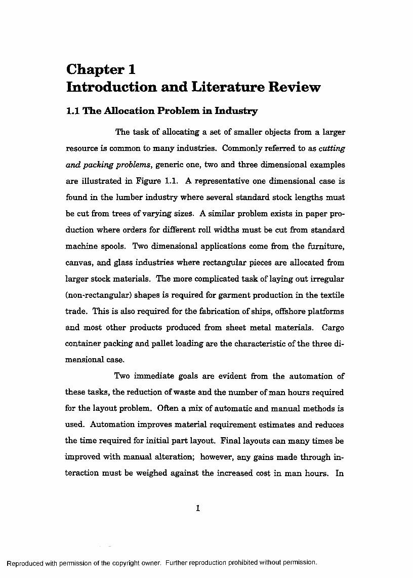
C hapter 1 Introduction and L iterature R eview1.1 The A llocation Problem in Industry

The task of allocating a set of smaller objects from a larger

resource is common to many industries. Commonly referred to as cutting

and packing problems, generic one, two and three dimensional examples

are illustrated in Figure 1,1. A representative one dimensional case is

found in the lumber industry where several standard stock lengths must

be cut from trees of varying sizes. A similar problem exists in paper pro

duction where orders for different roll widths must be cut from standard

machine spools. Two dimensional applications come from the furniture,

canvas, and glass industries where rectangular pieces are allocated from

larger stock materials. The more complicated task of laying out irregular

(non-rectangular) shapes is required for garment production in the textile

trade. This is also required for the fabrication of ships, offshore platforms

and most other products produced from sheet metal materials. Cargo

container packing and pallet loading are the characteristic of the three di

mensional case.

Two immediate goals are evident from the automation of

these tasks, the reduction of waste and the number of man hours required

for the layout problem. Often a mix of automatic and manual methods is

used. Automation improves material requirement estimates and reduces

the time required for initial part layout. Final layouts can many times be

improved with manual alteration; however, any gains made through in

teraction must be weighed against the increased cost in man hours. In


practice the problem requires optimizatiou of both material and labor

used.

Several other equally important criteria must also be consid

ered. These include, but are not limited to: scheduling constraints im

posed by stock material inventories, production scheduling, and the avail-

abihty of fabrication machinery [SPER79]. Manufacturing equipment can

impose other geometric limitations on the layout, such as requiring guillo

tine cuts or additional spacing between profiles to account for the curf of

fiame cutting devices. Even with these restrictions, automation when im

plemented properly can help reduce overall production costs.

2-D

3-D

Figure 1.1 Three examples demonstrating the one, two and three dimension aspects of the allocation problem.


The work presented in this dissertation deals with a general

case of the two dimensional allocation problem, often called nesting. Al

though capable of dealing with less complex forms, the focus of interest

was on solving problems involving complex shapes. The objective was to

generate layouts automatically, based on reasoning about the part and

stock shapes involved. The technique developed is conceptually similar to

the manual method used in solving jigsaw puzzles.

Before detailing the actual focus of this project, a brief over

view is provided in the next section, of the various attributes used to

characterize and classify the numerous problems found in industry. The

particular class of problem studied in this work is then described and a

brief history of the project given. The remainder of the chapter is devoted

to reporting on previous attempts at solving this problem in the litera

ture. Finally, the proposed technique is discussed in light of this previous

research, and an outline of the remainder of the dissertation is given.

1.2 C lassification of A llocation Problems

Numerous techniques for automating cutting and packing

problems can be found in the literature. Much of this research is summa

rized in the surveys of Haessler, Sarin, and Hinxman [HAES91] [SARI83]

[HINX80]. However, Dychhoff goes one step further and proposes a typo

logy of all allocations problems based upon their fundamental logical

structure [DYCK90]. The purpose of the typology is to provide a consis

tent and systematic approach for condensing the myriad of problems in

vestigated, and to unify the different notions used throughout the litera

ture. This concept was expanded upon in the book Cutting and Packing

in Production and Distribution, A Typology and Bibliography, where four


general problem types were defined [DYCK92]. Since the goal of the book

was to serve as an aid in selecting and developing solution procedures,

these types have similarities in solution approaches. The problems asso

ciated with each type are described using entries firom a catalogue of

problem characteristics or attributes. The object in defining the four

types was not to use all attributes, but only those which are significant in

terms of solution procedures. Some of these "type-defining" characteris

tics are summarized next.

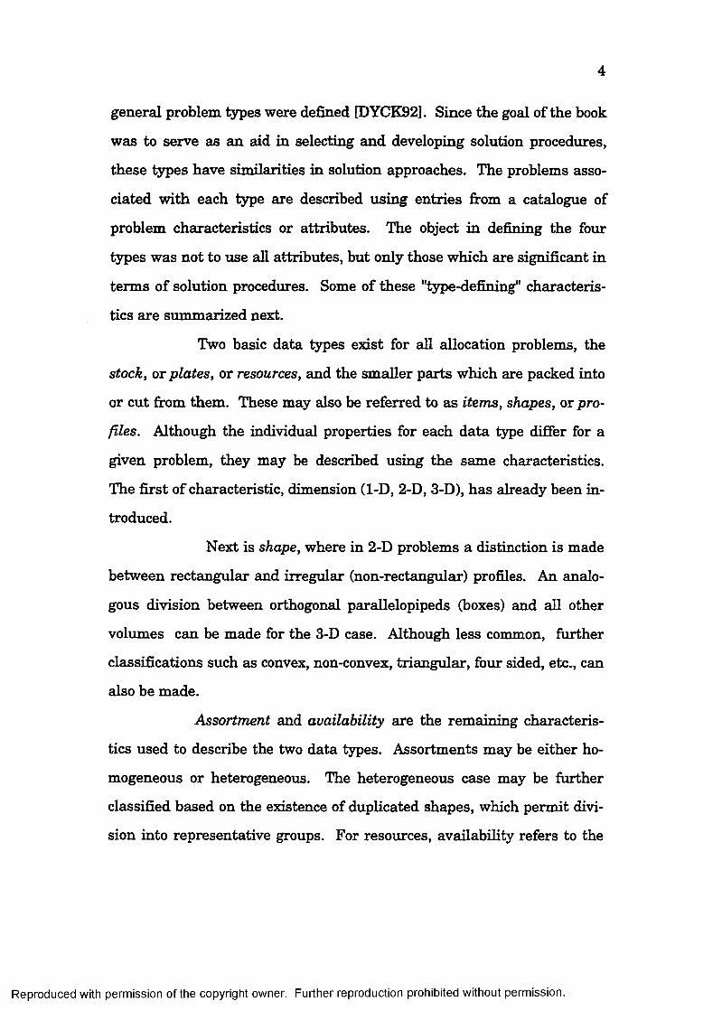
Two basic data types exist for all allocation problems, the

stock, or plates, or resources, and the smaller parts which are packed into

or cut firom them. These may also be referred to as items, shapes, or pro

files. Although the individual properties for each data type differ for a

given problem, they may be described using the same characteristics.

The first of characteristic, dimension (1-D, 2-D, 3-D), has already been in

troduced.

Next is shape, where in 2-D problems a distinction is made

between rectangular and irregular (non-rectangular) profiles. An analo

gous division between orthogonal parallelopipeds (boxes) and all other

volumes can be made for the 3-D case. Although less common, further

classifications such as convex, non-convex, triangular, four sided, etc., can

also be made.

Assortment and availability are the remaining characteris

tics used to describe the two data types. Assortments may be either ho

mogeneous or heterogeneous. The heterogeneous case may be further

classified based on the existence of duplicated shapes, which permit divi

sion into representative groups. For resources, availability refers to the


number of stocks accessible during the solution process, while for parts

availabiliiy defines the upper limit on items used or produced. Cases

with infinite stocks and/or parts occur firequently in industry.

Cutting and packing problems may also be characterized

based on the nature of the assignment involved. Dyckhofif enumerates

four types:

Type I: All resources and parts used,

Type II: All resources used, a selection of parts used.

Type HI: All parts used, a selection of resources,

Type IV: A selection of parts and resources.

Type I is a pure layout problem as when a set of machinery must be dis

tributed over a factory floor. For type II assignments, a selection of the

available parts is required to efficiently use all resources. Conversely, for

Type m all parts m ust be allocated with emphasis often placed on select

ing the minimum resources required. Type IV is a mix of both II and III.

The objective in carrying out assignments is also an attrib

ute describing the problem. The key goal is always focused on reducing

waste or maximizing profits; however, the exact criteria differ fi'om prob

lem to problem. Less obvious issues such as lowering inventory storage

and handling costs, and minimizing change-over and cutting times may

also come into play.

Geometric restrictions placed on the arrangement of parts

constitute yet another factor describing the allocation problem. For the

majority of cases, parts may not overlap and must fall totally within the

resource. Restrictions upon the orientation of profiles can exist due to di

rectional properties of the stock, as is the case for wood, milled steel, and


many composite materials. The fabrication equipment may also place

limitations on the patterns used. Arrangements where part boundaries

are parallel to stock boundaries (orthogonal patterns) are often required

for paper cutting devices. The ability to perform straight uninterrupted

cuts from one end of the resource to the other {guillotine cuts) is com

monly seen in this industry (Figure 1.2). Often, when processing sheet

metal, spacing between parts must be allowed to account for the curf of

the cutting device. Defects in the material itself can also affect the layout

patterns.

Dyckhoff also distinguishes four basic problem types, dis

tinct from the four assignment types mentioned earHer, based on the

CUT 2

CUT1

CUT 3

Figure 1.2 Different layout or pattern types: (a) guillotine, (b) nonguillotine or nested, (c) non-orthogonal.


above criteria: cutting stock, bin packing, knapsack, and pallet loading.

Cutting stock problems consist of large heterogeneous assortments of

parts with only a few distinct shapes which must be allocated to a selec

tion of stocks either completely or incompletely. Since the items may be

divided into a groups of identical shapes, repetitive solutions can often be

used for each resource. By contrast, the bin packing type also contains

large heterogeneous assortments of parts, but multiple identical parts are

not common. Consequently, this type of problem is more complex, as as

signments for each part and solutions for each resource must be consid

ered individually. In knapsack problems, a large, often infinite supply of

heterogeneous patterns must be assigned to a limited set of stock. For

this type of problem, all resources must be used to complete the solution.

Finally, the pallet loading type consists of problems where a selection of

homogeneous parts must be assigned to a generally homogeneous set of

stocks.

1.3 The Problem Investigated

The problem investigated represents a special case of the

two dimensional bin packing type often called nesting. The assortment of

parts is variable in nature. Profiles vary firom rectangles to highly irregu

lar and complex shapes involving chamfers, fillets and general curved

edges. The distribution of profiles is not characterized by multiple identi

cal copies and thus effectively eliminates the repetitive use of layouts as a

solution. There is no orientation restriction on the placement of parts.

The problem is further generalized by the requirement that, where possi

ble, items allocated be placed within the irregular holes or void regions

existing within some larger part profiles. All other resources or stock


8

materials specified by the user are rectangular. Various sizes and grades

are permitted, however the task of selecting the optimum stock is not ad

dressed [GEMM92] [QU89I.

Research for this project was initiated by a request firom a

ship and offshore oil platform fabricator seeking to automate material re

quirement estimates for large projects. Proprietary systems are available

firom CAMSCO and Gerbers Scientific for ship building while Micrody-

namcis, Assyst Inc., Inverstronica and others offer products for the textile

industry. None of the commercial packages satisfied the particular re

quirements of this project. Furthermore, such algorithm s are proprietary

and could not easily be incorporated into the sponsor’s current operations.

A one year pilot study was intiated and algorithms were developed to ad

dress the problems of interest. The results of this initial study are found

in Chapter two. Following this, an independent investigation was con

ducted to develop a new, more innovative, and efficient solution to the

problem. Although the majority of the research presented was conducted

during this phase, many of the strategies introduced were motivated by or

grew out of the results of the pilot study. Solutions fi'om the initial study

were also used as a basis of comparison for the new technique.

1.4 C lassification of Solution Techniques

Irregular profile bin packing falls into a class of problems

which are NP complete [GARE791. An infinite number of solutions are

possible and it is seldom possible to determine a true best solution for any

given set of patterns. In the absence of an analytically defined optimum,

a suitable goal for automation is a set of solutions equal in quality to

those of manually produced layouts.


Solution strategies for this type of problem can be separated

into two broad tasks, part selection and part placement. Part placement

focuses on identifying locations and orientations for profiles that satisfy

the geometric restraints imposed on the solution. This is often referred to

as layout or (cutting) pattern generation. Part selection or assignment

deals with choosing the best parts for each stock plate in the solution.

An interesting and familiar analogy can be found in the

game of chess. Here the generation of part placements is a relatively sim

ple task. A limited set of permissible moves for each piece are expHcitly

defined by a set of easily evaluated rules. For example, bishops may only

move any unobstructed distance along a diagonal, while rooks are re

stricted to purely horizontal or vertical movements. For the layout prob

lem, an infinite number of locations and orientations are available for

each of many parts, while the non-overlapping constraint makes validat

ing a placement substantially more complex. As with chess, selecting the

best move or placement is very difficult. Often parts are selected and

placed in an iterative fashion as with chess moves. For such an approach

it is often difficult to predict with certainty the future effect which any

placement may have on achieving the overall objective of the problem as

the number of possibilities is infinite- While preventing the capture of

the king in chess is difficult, optimal packing of highly irregular shapes is

an equally daunting task. Nor can the tasks be considered independent.

The interrelation between the layout and assign m en t is critical, as opti

mal selection of parts is rendered m eaning less without proper placement.

A review of the literature shows limited research into this

problem. In Dyckhoffs bibliography only 23 of the 142 two dimensional


10

problems cited involve irregular shapes. The majority of these are cutting

stock types. Due to the inherent complexity of nesting, almost all solu

tions employ some form of heuristic. The previous research can most eas

ily be classified based upon the method in which part placements are gen

erated. Using this method, three broad categories can be defined: 1) rec

tangular approximation strategies; 2) optimization methods; and 3) rule

based, intelligent or expert system approaches. Each group is detailed

further in the following sections.

1.4.1 R ectangular Approximation Placem ent Strategies

These methods reduce the complexity of handling irregular

profiles by approximating either individual or groups of parts with rec

tangular enclosures. With all pieces resolved to this form, the algorithms

for nesting rectangular shapes are directly applicable. As previously

mentioned, substantial research has been conducted in this area

[HAES91].

Much of the earliest work on the rectangular two dimen

sional allocation problem is credited to Gilmore and Gomory, who showed

that it could be formulated as a linear programming problem [GILM65].

Unlike the one dimensional case, the two dimensional problem could not

be solved using a knapsack function, as efficient solutions to higher order

knapsack problems were not available. However, with certain restric

tions, such as guillotine cuts, algorithms for optimal and near optimal so

lutions could be formulated. Since then other techniques have been used,

including: recursive algorithms, dynamic programming, combinatorics,

and various heuristics [ISRA82]. A representative set of these methods

may be found in references by Adamowicz, Bengtsson, Christofides, Dagli,


11

Dietrich, Farley, Hahn, Nee, and Oliveira [ADAM76], [BENG82],

[CHRI77], PAGL88], [DIET91], [FARL90], [HAHN68], [NEE88],

[OLIV90].

In their simplest form, rectangular approximation methods

replace each part profile by its minimum enclosing rectangle (MER) or

smallest bounding box. Efficient methods for generating a polygon’s MER

are detailed by Freeman [FREE75a] and Adamowicz [ADAM79]. The

quality of the nests produced is dependent to a large extent on the

accuracy of the MER; as all waste associated with this approximation is

automatically included in the solution. For highly irregular shapes this

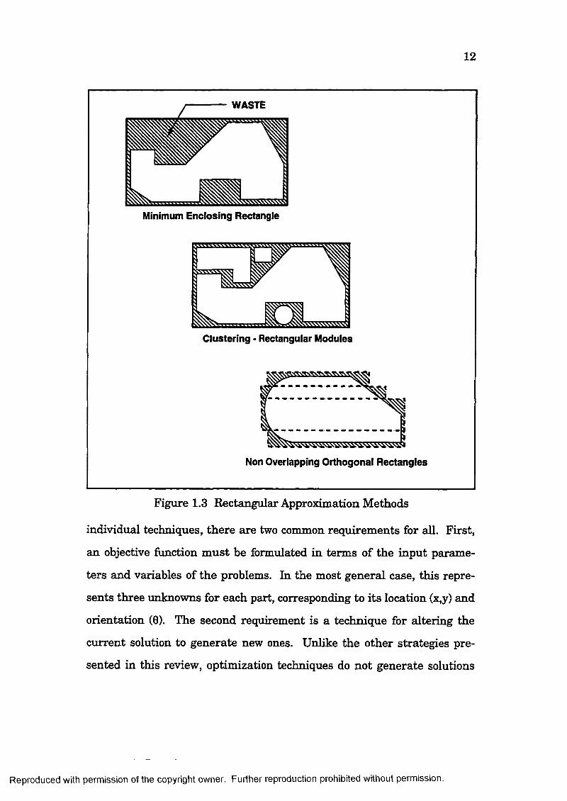
waste can be significant (Figure 1.3). In order to partially overcome this

limitation, some have proposed clustering pieces together to form rectan

gular modules which are subsequently nested [ADAM79], [NEE86],

[HAIM70]. This reformulates the problem as a series of smaller layouts,

since generation of each module is, in essence, the placement of pieces

onto a smaller resource. To be effective, this technique requires parts

which readily combine to form rectangles. Small parts are often required

to fill the waste areas encompassed by the rectangular enclosure. For

many applications these conditions cannot be met. Furthermore, parts

which are large relative to the available resource can not be clustered.

1.4.2 O ptim ization M ethods

The second group of approaches proposed in the literature

make use of several optimization techniques for minimizing trim waste,

including multi-start non-gradient searches, neural networks [POSH90],

[CAVI89], simulated annealing [DAGL90a], [DAGI90b], [KAMP88], and

genetic algorithms. Although implementation issues differ with


12

WASTE

Éwss'sswaMinimum Enclosing Rectangle

Clustering • Rectangular Modules

Non Overlapping Orthogonal Rectangles

Figure 1.3 Rectangular Approximation Methods

individual techniques, there are two com m on requirements for all. First,

an objective function m ust be formulated in terms of the input parame

ters and variables of the problems. In the most general case, this repre

sents three unknowns for each part, corresponding to its location (x,y) and

orientation (0). The second requirement is a technique for altering the

current solution to generate new ones. Unlike the other strategies pre

sented in this review, optimization techniques do not generate solutions


13

through the iterative placement of individual parts onto the resource.

Rather, some initial solution including all parts is improved through vari

ous perturbation methods.

1.4.2.1 The Objective or Cost Function

The objective function may be formulated in several ways.

However, when minimized it must generate solutions conforming to the

geometric constraints imposed on the system. Since most applications re

quire non overlapping placements, one term representing the area of in

tersection between parts can be found in almost all cost functions. Deter

mining this term constitutes the majority of solution time, thus various

methods for its efiScient calculation have been proposed. If only an ap

proximate measure is desired, a quadtree approach, as presented by

Sandgren, may be used to achieve any desired level of accuracy

[SAND88]. However, computation expense increases as the m inim um

grid size used to describe profiles decreases. A more analytical approach

for finding the exact area of intersection is demonstrated by Jain

[JAIN92]. Results firom computational geometry show that calculation of

the overlap between two polygons with N sides requires on the order of

time [PREP85]. Consequently, as the number and complexity of parts

increases, the expense of calculating this term can become substantial.

Beyond preventing overlap, a term controlling the overall

size of the layout must be present in the objective function to reduce the

resulting trim waste. If the dimensions of the used resource are uncon

strained, the area of the rectangle encompassing all patterns is mini

mized. A useful alternative is to minimize the sum of the distances be

tween each profile and the origin. For most other cases where the stock


14

material is of a set width, the appropriate restrictions are applied to the

layout and overall length is controlled. The following metric, D, may also

be minimized

^ [11] P i

where

djj = the distance between parts i and j,

w - = the afBniiy or attraction of part i for part j.

Various bases for calculating the attraction of one part for another may be

measured such as maximum edge-wise adjacency or the area of the small

est enclosing rectangle for the various part pairs. The desired goal of

such terms is to help drive the optimization method toward effective part

placements and layout solutions.

One difficulty in solving the allocation problem using an op

timization formulation is the potential for numerous local m inim a in the

cost function. Two strategies exist to overcome this problem. In multis

tart methods, the random selection of many starting points allows for the

location of the different local minima. The smallest result is chosen as

the global minima. If this technique is used, traditional "downhill" search

algorithms can be used to improve the layout. However, due to the non-

differentiable nature of the objective function, non-gradient based tech

niques are generally required. The second approach is to choose a search

capable of "jumping out o f the valleys associated with local m inim a, such

as simulated annealing or genetic algorith m s.


15

1.4.2.2 Sim ulated A nnealing Techniques

Simulated annealing is a "probabilistic hill climbing optimi

zation technique" [JAIN92] [KIRK83]. The basic steps for implementing

a simulated annealing algorithm are shown in Figure 1.4. The overall

structure consists of two loops. Within the inner loop, the current con

figuration or layout is altered in a random fashion to produce another

configuration kj within its neighborhood. The layout generated may be

accepted based on one of two criteria. If the cost of the objective function

for kj is less than or equal to that of it is accepted. Otherwise, the ac

ceptance of kj is based upon the generation of a random number between

zero and one. If this number falls below:

[1.2]

where

àC = C(kj)-C(k^ [1.3]

and C( ) represents the value of a configuration’s cost function, kj is ac

cepted and becomes the current configuration. Otherwise the original

configuration is retained. Processing within the inner loop continues un

til equilibrium is reached, which for nesting applications is usually de

fined as the generation of a preset number of accepted configurations.

The algorithm then jumps to the outer loop where the controlling parame

ter or temperature, T, is decremented. Processing continues in this way

until the temperature is small enough to prevent any substantial im

provement to the solution. The key advantage of the method is its ability

to accept intermediate solutions with higher cost values in a controlled

way.


16

Various techniques have been used to generate the neces

sary intermediate layouts, which are often referred to as moves. One

method is to interchange the position of two objects [LUTF92]. More typi

cal, however, is the random perturbation of a part’s position (x,y) and ori

entation (0). Since the new configurations must fall within the

RAND

Decrement T

END WHILE

Generate an Initial Configuration k.

WHILE Not in Eqilibrium

Generate a New Configuration through a random perturbation of kj

Figure 1.4 Flow diagram showing the basic steps of simulated annealing


17

neighborhood of the old configurations, the magnitude of change is usu

ally limited. In most implementations, as the temperature is lowered, the

extent of part movement is reduced, causing a corresponding reduction in

the size of the associated neighborhood.

A cooling schedule specifies the way in which the tempera

ture is decremented and determines the criteria for equilibrium at each

stage. Proper selection of the cooling schedule is critical. If the initial

temperature is set too low or cooling proceeds too fast, the solution may

be trapped in a local minima. If the temperature is set too high and dec

rements too small, the method will progress unnecessarily slowly. Selec

tion of the cooling schedule is usually done by trial and error based on in

formation gained firom prior runs with a similar structure.

1.4.2.3 Genetic Algorithm s

Another probabilistic approach to solving the nesting prob

lem is to combine genetic algorithms with a local minimization routine

[FUJI93]. In order to handle solutions in a manner analogous to genes,

layouts must be formulated as strings. For this purpose, solutions are

represented as an ordered list of parts (e.g. part A, part B, . . ., part J).

The location of each part in the layout is measured in the local coordinate

system of the pattern immediately proceeding it in the list. A set number

of such solutions is generated to start the process. At each stage of the

algorithm, a fitness is assign to each member of this population of layouts.

This fitness number corresponds to the value of the cost or objective func

tions mentioned previously. At each stage of the solution, a new genera

tion of layouts is produced fi*om those members having the highest fitness

values, using three of genetic operators.


18

The three genetic operators used represent techniques for

generating new solutions from the current generation of layouts or idi-

viduals. The first and most frequently used operator is ordered crossover.

A pair of individuals labeled parent 1 and parent 2 are selected and a

crossover location in the ordered lists, representing their solutions, ran

domly selected. A child or new solution is produced in the following fash

ion. The portion of parent 1 lying to the left of the crossover point is

copied directly into the child. The remaining profiles are copied into the

child in the order in which they appear in parent 2 (Figure 1.5). The rela

tive coordinates (x,y,0) of each part are retained from its parent string

with one exception. The coordinates of the part immediately following the

crossover location are generated randomly. A second child can also be

produced by exchanging the roles of parent 1 and parent 2 and repeating

the process. The second genetic operator used is mutation. Here a ran

dom piece is removed from the solution and re-inserted at a random loca

tion in the list (Figure 1.5). For the final technique, elitist selection, a

child is produced by copying the solution with the highest fitness directly

into the new generation. The probability with which the three operators

are applied is preset in the algorithm.

The solutions produced in the above fashion are seldom ac

ceptable layouts. Consequently, a local minimization must be performed

on each of the children. Analogous to multistart methods, overlap and

layout dimensions are minimized using a "Quasi-Newton" method. The

square of the distances between adjacent parts in the solution Lists is also

minimized. This overall process is continued until a set number of


19

generations has been produced. The member of the population with the

highest fitness is selected as the final solution.

Crossover Location

Parent 1: +A +B +C +D +E +F +G +H +1\ ■ y

Parent 2: -I -A -D -F -H -C •B -G -E

Child 1: +A +B +C +D +E =1 -F -H -G

(a )

' Removed PieceChild :

Mutated Child :

+A +B +C +D +E =1 -F 1 -H -G

t t t t t+A +B +C +E =1 -F +D -H -G

( b )

+ Relative position inherited from Parent 1 - Relative position inherited from Parent 2 = Random relative position

Figure 1.5 Operators used in the genetic algorithm: (a) Crossover, (b) Mutation

Although computationally expensive, optimization tech

niques offer the advantage of potentially finding a true m inim um over the

range of design variables. Unfortunately, the computation time associated

with such solutions are often impractical. For example, the genetic algo

rithm referenced above required 12 hours to nest 12 parts. As a


20

consequence, problem formulations are often limited to either relatively

few parts or only convex patterns. Although such limitations are applica

ble to certain stamping operations, they cannot be reconciled to the prob

lem of interest. Furthermore, no method for dealing with resources of

limited dimension has been proposed.

1.4.3 R ule Based, In telligent, & Expert System s

The ftnal group of solutions to the irregular 2-D bin packing

problem are lumped into a category referred to as rule based, intelligent

and expert systems. Although broad, all methods in this class differ from

those solutions previously presented in two key ways. First, unlike rec

tangular approximation strategies, irregular geometries are used to rep

resent the parts during placements, and second, solutions are generated

by placing parts onto the resource one at a time in a sequential fashion.

This differs from optimization strategies where a layout for all parts is in

itially present. Consequently, a t each stage of the solution process, an in

finite number of positions and orientations exist for those parts remain

ing to be placed. To reduce the possibilities to a reasonable number of

choices, various heuristics are incorporated.

1.4.3.1 F ixed O rientation Boundary Abutting Techniques

Much of the variability in placement of parts can be reduced

by restricting the number of different orientations allowed for profiles.

No clear automated method for picking the optimum orientation exists,

however efficient selection can often be done manually. With profiles con

fined in this way, satisfactory positioning can often be achieved by placing

parts such that they touch but do not overlap.


21

Various methods for generating these placements are found

in the literature. Freeman outlines a procedure for packing a single

arbitrary shape multiple times; however, the profiles must first be ap

proximated using a chain code [FREE75b], An interesting hybrid of the

rectangular approximation schemes is presented by Qu [QU87]. Each ir

regular profile is represented by a set of non-overlapping orthogonal rec

tangles (Figure 1.3). Adjacent and non-overlapping placements are easily

determined since intersection of the component rectangles is a straight

forward process. Packing proceeds by producing a series of stock width

sized strips or layers which are then used to fill the resource firom top to

bottom. Although promising, this profile approximation technique re

stricts the final solution to orthogonal layout patterns. Furthermore, a

part’s representation is highly dependent on orientation. Even some rela

tively simple shapes can require a large number of rectangles for effective

approximation, causing the approach to be computationally impractical.

The most general fixed orientation boundary abutting ap

proach was presented by Albano and Sapuppo [ALBA80]. A geometric

construct, referred to as the No Fit Polygon, is used to determine the lo

cus of all points where a part may be placed such that it touches but does

not overlap any already allocated part. Unlike other placement tech

niques, any polygonal representation of the parts can be used for calcula

tions. By combining this method with a "placement pohcy" and a search

heuristic, an effective method for solving the irregular bin packing prob

lem was produced. A logical extension of this technique to more general

problems was developed in the initial phase of this project. A more


22

detailed discussion of the pilot study is deferred until Chapter 2, where

the results are presented.

1.4.3.2 Shape Based Techniques

A key drawback of the techniques presented in the previous

section is the limitation of the number of orientations which parts may

take in order to reduce computational expense. Frequently only integer

multiples of tc / 2 are investigated (0®, 90°, 180°, 270°); however, even for

rectangular shapes, these may not produce optimal nests [DECA78].

A more "intelligent" approach for selecting, orienting, and

placing parts is to mimic one technique used by manual nesters. Here a

search is conducted for complementary shapes among the unplaced part

profiles, and the remaining usable stock profile. Solutions are generated

by piecing together layouts in a puzzle like fashion. Reasoning of this

lype has been proposed to varying degrees by several authors.

In the most elementary form, shape reasoning represents the

matching of profile sides. This is the approach taken by Dagli and Toto-

glu [DAGL87]. Patterns are allocated to plates sequentially, with the or

der determined by a set of priorities based on properties such as part

area, profile perimeter, and complexity. Starting with the two highest

priority parts, their relative locations are determined by pairwise match

ing each of their sides (Figure 1.6) and selecting the location yielding the

smallest minimum enclosing rectangle (MER). The process is repeated

with the next part profile in the prioritized list until all parts are placed,

or no more room is available to place additional parts on the existing re

source. The indiscriminate checking of all possible combinations of sides

incurs the largest computational expense associated with the algorithm.


23

This basic principle of matching sides is used in another al

gorithm discussed by Prasad [PRAS94], One part is held hxed while the

other is slid or translated along its boundary as in the no fit polygon

(NFP) described by Albano and Sappupo [ALBA80]. The orientation of

the parts is determined by aligning the longest edges of their correspond

ing profiles. An MER is then constructed for each step of the NFP proc

ess. As with Dagli’s method, the placement corresponding to the smallest

MER is selected as best. Unfortunately, this algorithm is designed for

MER

Figure 1.6 The method of Dagli and Totoglu. Part placements are generated by pairwise matches of all sides of parts A and B.The location producing the smallest MER is selected as best.


24

sheet metal stampings, and is limited to problems of only two or three

parts.

Rule based or expert systems represent a second category of

approach using shape to solve the nesting problem. One example, devel

oped for a ship building application is presented by Cheok and Nee

[CHE091]. The automatic layout process is divided into three steps. In

the first stage, called shape processing, an approximate description of the

part profiles is produced by eliminating fillets, chamfers, and other minor

features. These simplified shapes are then classified into groups based on

commonly used parts such as floors, rectangular brackets, trapezoidal

brackets, etc. (Figure 1.7). In the second stage, the classified parts are

paired together according to predefined arrangements which, based on

previous experience, produce "good" or tightly packed rectangular

modules. These modules are nested in the third stage using a specialized

rectangle packing method.

A second example of a rule based method is discussed by

Yazu [YAZU87], where the shapes are based on clothes patterns. A large

set of specific rules is used for each clothing type, such as men’s shirts.

Details concerning these rules and their use are not clearly presented in

the discussion.

A key limitation of rule based techniques is their domain de

pendency. That is, they are very case specific. Consequently, the heuris

tics often break down in the context of general nesting, where unexpected

situations occur, causing undesirable results.

A familiar and interesting analogy to the nesting problem,

that of putting together jigsaw puzzles, was investigated by Freeman and


25

later by Radack and Badler [FREE64], [RADA82]. Radack and Badler’s

study determined matches based on a novel method for representing the

part profiles using a boundary-centered polar encoding. Freeman based

the correct placement of parts on comparisons between partial segments

or "chainlets" of the part profiles, chosen such that it was likely that there

would be only one mate with a chainlet firom any other piece.

Brackets (Trapeziodal)Brackets (Triangular)

Floors

Figure 1.7 Cheok and Nee’s rule based methods. Parts are classified into groups and packed into rectangular modules.

Chainlets were produced by dividing the part profiles at

"critical" points, defined as inflection points and slope discontinuities in

the profile [FREE78]. Since there are usually a high number of chainlets

and combinations possible, a rough measure of their sim ilarity is first es

tablished by comparing a set of orientation invariant measurable fea

tures. Examples of these "features" can be seen in Figure 1.8. This


26

information is used to determine the most likely matches, which were

then subjected to a more intensive comparison. The puzzle is assembled

by adding individual pieces to a core central piece. Thus the solution

grows in an outward direction.

The difficulty in applying the above approaches to nesting is

tha t exact puzzle-like profile matches seldom exist in practice. Therefore

many, but not all of the techniques discussed are of limited use.

Chainlet

9 Critical Points

Puzzle Part Profile Description

Distance VectorChainlet Features

• # of times Chainlet crosses Distance Vector

• Ratio of area on either side of Distance Vector

Maximum Perpendicular distance from Distance Vector

Figure 1.8 Several orientation invariant measures of shape or "chainletfeatures" used by Haims to solve the apictorial jigsaw puzzle problem. Chainlets are formed by dividing profiles a t critical points.


27

However, it will be shown that tiie use of features for rough shape com

parisons does have merit for the problem studied.

Perhaps the most comprehensive approach to solving the bin

packing problem using shape is outlined by Chung and his colleagues

[CHUN89]. A series of techniques is used to orient, place, and pack parts.

The primary basis for placement is a shape heuristic which attempts to

match concavities and convexities which exist in parts. For each parrt, a

best fitting adjacent piece is defined for each of its four primary (90°,

180°, 270°, 360°) orientations. At each stage of the solution, the best fit

ting adjacent piece associated with the last placed part is tested. Unfor

tunately, no information is provided on how these best fit pieces are de

fined, and whenever the best fitting piece logic fails, a more basic angle

heuristic is appfied.

The angle heuristic uses an approximate polygonal represen

tation of the irregular profiles, which must be provided by an experienced

technician. For each approximating polygon, a series of outer angles is

defined (Figure 1.9). Candidates for placement are determined by com

paring the outer angles of a part with those of the most recently placed

part. If the difference between angles falls below a threshold, tha t part is

considered for placement. The largest of the candidates is selected as the

next best fitting part. Placements are tweaked further by minor transla

tion and rotation. A quadtree approximation of the parts is used to deter

mine intersections and prevent overlap. Restricting parts to only four ba

sic orientations is the key limitation of this approach which is less detri

mental if nearly rectangular shapes are used. However, more complex


28

forms generally require additional freedom if effective placement is

desired.

The work presented in this manuscript represents an inno

vative solution technique for a general class of bin packing problems, us

ing original methods for dealing with and reasoning about shape. The

underlying objective behind this research is to go beyond simple edge and

angle comparisons to develop intelligent heuristics based on more infor

mative geometric characteristics. However, to be effective this must be

done while still dealing with shape at a rudimentary level, less case

Outer Angles 0.j_^

Abstract Polygon

Figure 1.9 Chung's method. Profiles are placed using the outer angles of the "abstract polygon" representing each part.


29

specific than contemporary expert systems. This is made possible by han

dling the placement ambiguities present in nesting while reasoning about

the solution in a way reminiscent of the puzzle problem. In the following

chapters, a methodology for incorporating these concepts into a compre

hensive nesting algorithm is presented.

1.5 D issertation Layout

The remainder of the dissertation is laid out in five chapters.

Chapter Two defines much of nomenclature used and summarizes the

work conducted for the initial study. Chapter Three outlines the funda

mental premise behind the proposed approach, and presents the basic ve

hicle used to describe shapes, features. Methods for extracting features

firom the geometries involved are also discussed. In Chapter Four, tech

niques for selecting and placing parts using features are demonstrated.

The technique was tested on a large set of industry supplied problems to

investigate its characteristics and evaluate performance. These results,

the overall structure of the solution strategy, and other important control

heuristics are presented in Chapter Five. The final chapter discusses

conclusions drawn fi-om the research and suggest possible avenues for fu

ture work.


C hapter 2 The P ilo t Study2.1 Introduction and Background

Interest in the 2-D allocation problem was initially gener

ated by a request from industry to automate material requirement esti

mates for large offshore platform fabrication projects. A one year pilot

project was conducted, and methods meeting the specific requirements of

such a commercial appbcation developed. Initially, a review of the cur

rently available techniques was conducted, seeking solutions with the

fimctionabty to deal with highly irregular shapes efficiently, and the abil

ity to nest on non-rectangular resources. Heuristic methods of the rule

based, intelligent and expert system type (§1.4.3) were best suited to this

task. Although none of the published techniques could address all con

cerns of the project, the method presented by Albano and Sapuppo

[ALBA80] was judged best suited for needs at that time. During this in

itial phase of research, Albano and Sapuppo’s technique was implemented

and its domain of application broadened to include the more general char

acteristics of the industry problems involved.

The work of the pilot study is described in this chapter. In

section two the method of Albano and Sapuppo is explained a t length. Al

though a more innovative approach is presented in later chapters, several

of the core elements and much of the terminology is shared with this tech

nique. In section three, the primary adaptation permitting the use of

non-rectangular stocks is detailed. Several aspects of the final solution

strategy evolved from the way in which this modification was addressed.

30


31

Next, profile simplification algorithms and other techniques used to pro

duce effective and computationally efficient representations of complex

parts are presented. Finally, the overall implementation is described and

its limitations discussed.

2.2 The M ethod o f Albano and Sapuppo

As with most rule based, intelligent and rule based systems,

the method of Albano and Sappuppo attempts to mimic the methods used

in manual nesting. Final solutions are built by placing parts onto the re

source one at a time. Two basic tasks exist for such an approach: part

placement and part selection (§1.4). Part placement focuses on identifying

the best location and orientation for a new part such that it generates a

minimum amount of waste and does not overlap any existing parts, while

part selection deals with choosing the best part to place at any given step

in the solution process. The approaches used to address each task are

presented separately in the following two sections.

2.2.1 Part Placem ent

Although determining non-overlaping positions is an impor

tant restiction during part placement, it is usually only the m inim um re

quirement. In general the placement which will generate the least waste

or trim is desired. Such a placement can often be achieved using a con

struct called the No Fit Polygon (NFP) [ALBA80]. By definition, the NFP

between two parts A and B is the locus of all points where the reference

point of part B may be placed such that B is touching but does not overlap

A. In a more general sense, the NFP can be thought of as the path traced

by the reference point of part B, as it translates or slides (not rotates)

around part A (Figure 2.1). The reference point may be any location on


32

the part. For simplicity, a vertex of the part profile is generally selected.

This causes no loss of generahty, as selecting any other point will simply

translate the NFP relative to B without changing its form. Two algo

rithms for constructing an NFP were found in the literature.

ReferencePoint Step 1 Step 2

steps Step 4

Step 9 : No Fit Polygon

Figure 2.1 Generating a No Fit Polygon (NFP)

Lozano-Perez details a method for constructing the NFP us

ing the known properties of convex polygons and set sum operations

[LOZA83]. This formulation comes firom robotics and path planning

where non-intersecting positioning of objects is often of interest. If 12 is

an object, such as a robot, moving only by tran slation , and A is a


33

stationary obstacle, the set of positions for R avoiding A is the Minkowski

sum of A and i-R). The Minkowski or vector sum of two polytopes, P and

Q is the set [SERR82]:

P + Q {p + g I p is in P and g is in Q } [2.1]

where + is vector addition. If the two polygons involved are convex, there

is a simple algorithm for constructing the Minkowski sum. The orienta

tion (0) of each edge is recorded as the boundary of the two polygons are

traced in a counterclockwise direction. The list of edges for both polygons

is then sorted into increasing order of orientation and concatenated to

produce the NFP. A similar technique using successive applications of

the same algorithm may be used if the parts involved are not convex;

however, a convex decomposition of the parts must be known. This sub

stantially complicates the procedure.

A second technique for finding the NFP, described by Prasad

[PRAS94], works equally well with convex and concave parts and is the

method used in this research. Before outlining the algorithm, the conven

tions used for defining part profiles are discussed.

The profile for part A, P^, is defined by an ordered list of 2-D

vertices,

^2A> ^3 A ' ' ^ .2]

where N is the total number of vertices for tha t object. Vertices are coor

dinate pairs in the (x,y) plane, where

~ iA ' [2.3]All profiles are oriented such that part material lies to the left as the

boundary is transversed; thus, parts profiles are counter-clockwise. The

edges of profiles are represented by the notation E, where is the


34

directed vector from to ^ inward facing normal for each

edge i, , is defined as

^ lA ~ “ z ^

where is the unit vector in the positive z direction. It is also useful to

classify each vertex as either convex or concave. The following definition

is used.

i f ( X E ^ ) 'U^ > 0) I is convex

else

Vjj is concave [2.5]

When the meaning is clear from the context, the subscript "A" identifying

the part may be dropped from all of the above notation.

The NFP of part B with respect to part A is produced as B’s

profile slides along the stationary boundary of A in a counterclockwise

fashion. The path taken by part B’s reference point can be decomposed

into a series of steps which may be determined using the technique de

scribed below.

An initial position for B, such that it intersects but does not

overlap A, is provided by co-locating the leflmost lowest vertex of A with

the rightmost highest vertex of B. The intersection points are referred to

as the contact vertices and are denoted as

contact vertex A :

contact vertex B : CVg =

where i and j reference the appropriate vertex within the ordered list de

scribing each part profile (Figure 2.2). In this position two translation di

rections are possible for part B, such that it slides along but does not

overlap part A. The direction of movement, or movement vector S , is


35

given by

® ~ iA I ^JB ^ ~ ® [2.6]

otherwise

® = ~^jB

where the maximum distance of translation is indicated by the corre

sponding edge length of S.

To determine the extent of movement, a copy of the ray S is

extended from all vertices of B and the shortest distance to intersection

with an edge of A recorded (Figure 2.3). A similar procedure is applied

for the vertices of Part A. However, copies of -S are used, and intersec

tions with the edges of B are calculated.

Direction of Movement

Ss-E.

Initial Position

ContactVertex

Reference Point —

Contact Vertex B

B

Contact Vertex A

Figure 2.2 Initial positioning to generate the NFP between Parts A and B showing the direction of movement and contact vertices.


36

If no intersections occur within the prescribed limit, B is

translated by the maximum length possible, and depending on the move

ment vector used, one new contact vertex is identified from

= W [2.7]

or

The second contact vertex remains unchanged.

Copies of -Sfrom each Vertex of A

Copies of Sfrom each Vertex of B

Points of Intersection Copies of 5Closest Intersection Distance Length of Movement

After First Move

ContactVertex

First Segment of NFP ^

Figure 2.3 Determining the extent of movement at each stage as part BDetermining the of movement eachextent atmoves around part A in a counterclockwise direction.


37

When a valid intersection was detected along the movement

vector part B is translated by tha t distance dictated by the intersection.

The vertex from which the shortest movement vector S (or -S) was re

corded becomes the new contact vertex for that object. The location of the

intersection on the other part’s edge is also saved, and a new vertex in

serted a t that location. This point becomes the new contact vertex for

tha t part. A new direction of movement is formulated with these contact

vertices, and the process repeated until the reference point of B eventu

ally returns to its initial position.

Since more than two parts are normally involved in a layout,

part A may represent a single part profile as above, but is most often the

cumulative profile of all of the parts already placed on the stock sheet, or

merged profile (Figure 2.4). The merged profiles of layouts consisting of

numerous parts may become complex; consequently, a large computa

tional expense is incurred in determining the intersections between each

direction vector S and all edges involved. Several measures are

Merged Profile

Figure 2.4 A group of parts and their associated Merged Profile.


38

implemented to eliminate calculations, which are unnecessary based on

the non-manifold nature of the involved profiles.

All edges not facing the the movement vector may be elimi

nated, as a nearer intersection with some other edge of the part facing the

direction of motion is always guaranteed with closed profiles. Based on

reasoning analogous to that used in back face rejection hidden line re

moval algorithms [FOLE84], the edges of part A may be eliminated fi-om

intersection calculations using the metric

i f ( S ' < 0) I eliminate E ^ . [2.9]

Movement vectors may be eliminated if they point into the part, since, as

with the edges eliminated above, a closer intersection is always provided

by the remaining entities. Elimination of movement vectors is deter

mined by examining the vertex firom which they originate (Figure 2.5).

Two cases are possible. For the concave vertices of part B the criterion is

i f ( S ' ^ ^ ) OA ( S • > 0) I eliminate [2.10]

while for convex vertices it is

i f ( S ' N ç-_2JA ^ ^ ) AND ( S • > 0) | eliminate [2.11]

Similar criteria for the edges of part B and the vertices of part A may be

formulated by substituting -S for S in the above equations. The cost of

calculating the NFP can be substantially reduced in this way.

To position a new part B onto the nest such that it is touch

ing but not overlapping any of the existing parts, the reference point of B

will be placed somewhere on the NFP. A second condition, which must be

satisfied by B’s placement, is that it must fall totally within the bounda

ries of the resource or stock material. In order to meet this constraint,

the allocation region of part B on the resource is determined. The


39

allocation region for a part in a given orientation is simply the area in

which the reference point on B may be placed, such that B is contained

entirely within the resource. This area, shown in Figure 2.6, is easily de

termined for a rectangular resource, given the minininTn and maximum x

and y extents of the part relative to its reference point. By selecting a

point on the NFP which is contained in the allocation region, it can be in

sured that both conditions are satisfied.

r-• •

Before Eliminations : "11 Edges

After Eiiminations : ! ' ' “ •«rs6 Edges

Figure 2.5 Savings through elimination of edges and vertices during NFP intersection calculations

In practice, an NFP and allocation region must be calculated

for each candidate orientation of a part. For a given orientation, all

acceptable locations of the part are determined by finding those portions


40

of the NFP falling within the allocation region. This is done by clipping

the NFP on the rectangular boundary of the allocation region using a 2-D

Cohen-Sutherland algorithm [FOLE841, A placement policy is then used

to select the location which is most appropriate for this orientation. In Al-

bano and Sapuppo [ALBA801, a leftmost lowest placement policy was

applied, causing parts to be packed in the lower left-hand comer of the

stock plate. Other placement policies are equally valid. With a position

selected for each orientation, the placement policy is applied once again to

Allocation Region

Reference PointStock Plate

\ Leftmost Lowest Placement

/ t

NFP AA J NFP Falling within

Allocation Region

Final Part Placement

Figure 2.6 Part placement withing the allocation region


41

select that candiate with leftmost lowest extention. The quality of Üie so

lution generated depends greatly on the number of distinct orientations

tested for each part.

2.2.2 Part Selection

The other basic task of the nesting heuristic involves select

ing the most appropriate part for placement a t any given stage in the so

lution process. The tree structure of Figure 2.7 is a graphical representa

tion of the various possibilities. Nodes on the tree are referred to as allo

cations, and each represents an intermediate solution to the layout

problem. The level of an allocation is denoted by the number of placed

parts it contains. At each stage of the nesting algorithm, a new interme

diate solution or successor can be generated from any node containing un

placed parts.

Complete Allocation Tree (4 Parts)40 Intermediate & 24 Final Solutions

Level 0 :4 parts available Level 1 :1 placed / 3 avail. Level 2 :2 placed / 2 avail. Level 4 : Solution - Levei 0

- Levei1

-Level 2

- Level 3- Level 4

Figure 2.7 A complete allocation tree for 4 parts with only one orientation allowed.


42

A single part can produce an infinite number of successors to

a node, as each of its possible positions (x,y,0) will correspond to a new

intermediate solution. To reduce the total number of nodes, each part is

allowed to generate only one successor, corresponding to the placement

generated by the NFP / leftmost-lowest method of the previous section.

Even when restricted in this way, a large number of intermediate solu

tions can be generated firom even a small group of parts (Figure 2.7).

The majority of intermediate solutions are not of interest, as

only those nodes lying on a path between the initial and optimal final

node are necessary to generate a solution. The total number of intermedi

ate solutions produced can be substantially reduced if only these required

nodes are generated (Figure 2.8). Albano and Sapuppo propose a search

technique for transversing the allocation tree to produce such an optimum

search path [ALBA80].

Solution Tree with Optimum Search Path (4 Parts) 12 Intermediate & 1 Final Solution

Waste function values shown to demonstrate back tracking.

' ................................................................................ 48Back Tracking

0

- Level 0

Level 1

-Level 2

- Level 3- Level 4

Figure 2.8 A trimmed allocation tree showing the optimum search path


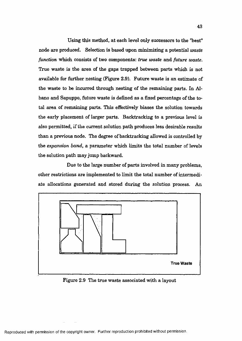
43

Using this method, a t each level only successors to the "best"

node are produced. Selection is based upon minimizing a potential waste

function which consists of two components: true waste and future waste.

True waste is the area of the gaps trapped between parts which is not

available for further nesting (Figure 2.9). Future waste is an estimate of

the waste to be incurred through nesting of the remaining parts. In Al

bano and Sapuppo, future waste is defined as a fixed percentage of the to

tal area of remaining parts. This effectively biases the solution towards

the early placement of larger parts. Backtracking to a previous level is

also permitted, if the current solution path produces less desirable results

than a previous node. The degree of backtracking allowed is controlled by

the expansion band, a parameter which limits the total number of levels

the solution path may jump backward.

Due to the large number of parts involved in many problems,

other restrictions are implemented to limit the total number of intermedi

ate allocations generated and stored during the solution process. An

True Waste

Figure 2.9 The true waste associated with a layout


44

upper bound on the number of successors produced a t each stage is set us

ing the parameter NJSUCCESSOR. The leftmost extension of each suc

cessor’s most recently placed part is used to determine which layouts are

retained. The number of intermediate allocations stored from previous

stages of the solution is also limited. These nodes are only of potential

use during backtracking; those extending beyond the expansion band are

automatically eliminated. Furthermore, only a set number

(MAXjCrENERATED) are retained based on lowest potential waste. A

more detailed explanation of the theory and implementation of the search

technique can be found in [ALBA80].

2.3 A daptations

In order to deal more effectively with difSculties encountered

in many industrial nesting applications, several substantial changes were

made to Albano and Sapuppo’s method. These extensions and enhance

ments produce better part placements, handle complex parts in a compu

tationally efiScient manner, and allow the technique to nest within voids.

Each of these improvements is detailed in the following sections.

2.3.1 Irregular R esourcesThe method described in the previous section is designed to

lay out parts onto an infinitely long rectangular stock. Added functional

ity is required if parts are to be nested onto finite resources with generic

irregular boundaries. Such situations occur in the production of leather

goods where animal hides are seldom rectangular, and may also occur in

the offshore platform and ship building industry, where small pieces are

often nested within the voids of larger parts to increase material usage.


45

New Part to be Placed

Reference Point

NFP of B on Merged Profile of Placed Parts

r T i

2

Allocation Region of B on Irregular Resouce

IrregularResource or Void

B2j

NFP of B on interior of Irregular Resource

NFP of B on Merged Profile, clipped on the Allocation Region

Leftmost Lowest Location on clipped NFP

Final Placement of B in leftmost lowest location

Figure 2.10 The method of Albano and Sapuppo applied directly to irregular resources. Note th a t the allocation region is the area enclosed by the NFP of B on the interior boundary of the resource.


46

If Albano and Sapuppo’s method is to be directly applied to

nesting on irregular resources, two NFFs must be calculated for each

part placement. As before, an NFP of the part on the merged profile of

all parts previously placed is constructed. In order to determine the

part’s allocation region, an additional NFP must be constructed on the in

terior boundary of the resource (Figure 2.10), since the simple bounding

box method used previously (§2.2.1) is no longer valid. Furthermore, clip

ping of the merged profile NFP is also more complicated as the new allo

cation region is no longer rectangular and may be non-convex.

The proposed heuristics for nesting on irregular resources

are similar to those used for a rectangular resource; however, the alloca

tion region and NFP are combined into a single construct called the Inter

nal No Fit Polygon (INFP). Analogous to the NFP, the ENFP is the path

traced by the reference vertex of a part as the part slides in contact with

the interior of a region such that the part is totally contained within and

is just touching the boundary. To effectively eliminate the construction

and subsequent clipping on the allocation region, the INFP must be per

formed on the remaining resource. The remaining resource refers to the

area within the void profile unused by the previously allocated parts (Fig

ure 2.11). The leftmost lowest placement now conveniently corresponds

to the leftmost lowest vertex of the INFP. With this new procedure for

placing parts, the strategy proceeds as before.

To construct the INFP using the same NFP algorithms dis

cussed earlier, two provisions m ust be made. First, the irregular resource

must be formatted as a part profile. The is easily accomplished by defin

ing the boundary such that material lies to the left as the profile is


47

transversed, as is needed with parts. If all irregular resources are viewed

as voids, this is achieved by a clockwise boundary orientation. Edges and

normals may then be defined as previously noted. Second, an initial

placement such that the part is totally contained within the void without

overlapping the boundary must exist. The original contact vertices re

quired to initiate the NFP algorithm, may be generated fi*om such a

IrregularResource or Void

New Part to be Placed

ReferencePoint

Remaining Resource or

Remaining Void

Internai No Fit Polygon ( INFP)

Leftmost Lowest Location on INFP

Final Placement of B in ieftmost lowest location

Figure 2.11 Part placement in voids using the Internal No Fit Polygon


48

position, by shifting the part until an intersection is found. If the void is

convex, the initial placement is simple to calculate. For non-convex

shapes, however, the initial placement selection is not as simple and a

decomposition of the void into convex regions is necessary. Candidate lo

cations are generated by a recursive subdivision algorithm as described in

Pavlidis and Feng [PAVL78]. The basic steps are:

(1) Determine all concave vertices of the void profile and the

distances between them.

(2) If non-adjacent, concave vertices exist, divide the region along

the line connecting the two closest non-adjacent concave

vertices. If only adjacent, concave vertices exist, divide the

region along the line bisecting the interior angle of one concave

vertex.

(3) Return to step (1) and apply the procedure recursively to the two

regions produced in step (2).

This process continues until all remaining areas are convex polygons (Fig

ure 2.12).

Initial placements for a part are determined by collocating

the center of the min/max box of the part with the centroid of a convex

subdivision. Due to the nature of the INFP construction method, necking

and small notches within the remaining void may cause some areas of the

resource to be inaccessible as the part slides along the boundary of the re

source. Consequently, each starting location may yield a distinctly differ

ent INFP and part placement (Figure 2.12). Therefore, the candidate re

gions corresponding to the desired placement policy Qeftmost lowest) are


49

tested first. To increase the likelihood of successful nonoverlapping in

itial placements, subregions with small areas and dissimilar min/max box

aspect ratios, relative to the part in question, are eliminated firom consid

eration. The initial location suggested may also be adjusted slightly when

only minor overlaps are detected between its profile and the boundary of

Part to be Placed

Current Intermediate Solution

e

t .Remaining Void —

0 Candidate Location C o Concave Vertex

y :e //' e

starting Location #1 (preferred)

1

Part may not pass from region #1 to region #2 p due to necking

Starting Location #2

Figure 2.12 Generating Initial Placements through convex decompositon


50

the void. Once totally contained within the void, construction of a vahd

INFP is assured.

2.3.2 Part Sim plification

Calculation of NFP*s and XNFPs can account for 80 to 90

percent of the computational expense associated with this method of solu

tion. The processing time required for each of these constructs is a direct

function of the complexity of the profiles involved.

For the pilot study, profiles were restricted to circular arcs

and straight line segments. For convenience, all arcs were approximated

to a desired accuracy by inscribed or circumscribed chords as appropriate.

Within industry, profiles with greater than 60 to 70 line segments were

commonly encountered with even the coarsest circular approximations.

Parts of this nature significantly increase the computational expense of

the NFP calculations.

Most complex shapes can be reduced to simpler, approximate

forms without adversely affecting the quality of the nest produced. A part

simplification algorithm using a modified convex hull approach was devel

oped to achieve this goal.

Each part is processed by first constructing its convex hull

[BOWY93], which reduces the complexity of the object but is often an in

efficient approximation of the shape. This is easily demonstrated by the

example of an "L" shaped bracket, where substantial waste would be in

curred if the convex hull approximation were used GFigure 2.13).

Further simplification is achieved through analysis and al

teration of the concave region profiles. The boundaries of these regions,

which are exterior to the part but interior to the convex hull, are


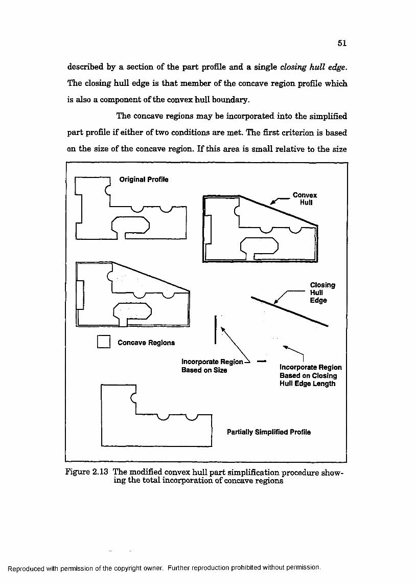
51

described by a section of the part profile and a single closing hull edge.

The closing hull edge is that member of the concave region profile which

is also a component of the convex hull boundary.

The concave regions may be incorporated into the simplified

part profile if either of two conditions are met. The first criterion is based

on the size of the concave region. If this area is small relative to the size

Original Profile

ConvexHull

ClosingHullEdge

I I Concave Regions

Incorporate Region Based on Size Incorporate Region

Based on Closing Hull Edge Length

Partially Simplified Profile

Figure 2.13 The modified convex hull part simplification procedure showing the total incorporation of concave regions


52

of the parts to be nested, the waste incurred by including it in the simpli

fied profile will be negligible. The second criterion is based upon the

length of the closing hull edge. If this length is small, it is unlikely that a

part could enter this region through the NFP placement mechanism.

When either condition is satisfied, the profile is simplified by eliminating

the original part edges associated with the concave region and replacing

them with the single closing hull edge.

Concave regions which cannot be incorporated into the ap

proximating profile using the two above criteria may still be simplified

using an approach similar to that used in finding initial placement loca

tions within voids. The area is recursively subdivided by lines connecting

closest concave vertices (Figure 2.14), as discussed earlier. These divid

ing lines are considered as closing hull edges and their associated areas

as "pseudo" concave regions. The appropriate dividing lines may be incor

porated into the simplified profile based upon the two elim ination criteria

previously given. A demonstration of the entire method is shown in Fig

ures 2.13 and 2.14. For this particular profile, the algorithm produces a

reasonable facsimile while reducing the complexity of the part by eighty

percent (down firom 33 to 6 edges).

2.3.3 Optim al Part O rientation

Another concern involving the NFP is the selection of part

orientations. For an optimal solution, all orientations of a part should be

tested, a proposition which is not feasible. The computational expense of

calculating an NFP for each orientation effectively eliminates this as an

option. For this reason, each part is limited to only four possible orienta

tions. Results fi'om the preliminary study indicate that aligning the


53

Partially Simplified Profile

Convex Vertices Dividing Lines Pseudo Concave Regions

Unsimplified Remaining Concave Region

Simplified Concave Region

Simplified Profile

Figure 2.14 The modified convex hull part simplification procedure show-convexing simplification of a concave region

part’s MER with the boundary of the rectangular stock is a good base ori

entation. The three other orientations are provided by successive ninety

degree rotations. For voids, a base orientation is provided by aligning the

part’s MER with the MER of the void boundary (Figure 2.15). The suit

ability of these orientations depends greatly upon the accuracy of the

MER.

As a finrther aid in placement, the foxor orientations of each

part are assigned a priority. Normally a best placement is determined by


54

Part Profile as Defined

Primary Orientation for Nesting

Region

Primary Orientation for Nesting within Void

Figure 2.15 The primary orientation for nesting within voids

that orientation causing the leftmost lowest extension of the part, as dic

tated by the placement policy. In many cases, however, all orientations

yield essentially the same positions based on this criterion. In such situ

ations (Figure 2.16), orientation priorities are used.

Preferences are established by calculating the above and

right areas of the part in each of its primary orientations. These areas


55

0“ (preferred) 1 90°

mé

180° 2 7 0 °

9 0°

1st Preference 2nd

180° 2 7 0 °

I3rd 4th

Figure 2.16 Four orientations produce the same leftmost lowest placment. Orientation priorities are used to select the best placement,

may be viewed as rough measures of the shadow cast by a light projecting

either from the right or above the part. The right area of a part is found

using its rightmost highest and rightmost lowest profile vertices. The

part profile is projected horizontally backward from these points until the

left most extension of the part is reached, and the area of the enclosed

polygon calculated (Figure 2.17). A similar procedure for constructing the

above area may be formulated using the highest rightmost and highest

leftmost vertices and projecting downward. For a leftmost lowest

placement policy, highest priority corresponds to that orientation

producing the smallest right area, while second preference is based on the

smallest above area (Figure 2.16). These heuristics aid in producing an


56

acceptable placement candidate while limiting the number of NFP’s cal

culated to four for each part.

Rightmost Highest Profile Vertext

^ Rightmost LowestProfile Vertext

Right Cast Shadow

Right Area

Highest Leftmost Profile Vertext

Highest Rightmost Profile Vertext

Lower Extent of Part

Above Cast Shadow

Above Area

Figure 2.17 Above and left area calculation technique.


57

2.4 P ilo t Study Summary

The solution method described was implemented and tested

a t an industrial marine fabrication facility. With the exception of input

and output file specifications, the package was totally automated. A brief

description of the application’s basic structure is provided to demonstrate

how the various techniques are integrated into a complete solution algo

rithm. A more detailed discussion of implementation issues and sample

nests is deferred until Chapter Five, where results of the primary tech

nique proposed in this manuscript are compared with the methods of this

chapter.

Processing begins with the sorting of parts into groups of

similar thicknesses and material grade. Prior to nesting each part is sim

plified and offset by a specified amount to account for the curf of the

flame-cutting device. Internal voids are also extracted for possible use as

irregular resources. These void areas are nested upon first, using the

INFP method. All remaining parts are then allocated to rectangular re

sources through the traditional NFP technique. Finally, the internal

voids and any associated nests are re-inserted onto their parent parts and

output files generated.

Results from the NFP/INFP application were acceptable in

light of the pilot project objective of producing material estimates for

large projects. In addition, the solutions generated also provided initial

nests as input to the company’s own interactive nesting system. These

layouts, however, could regularly be improved through manual modifica

tion. Several limitations of the NFP method became evident while


58

attempting to develop a new solution technique capable of improving the

results comparable to the manual tweaking.

One major drawback of the NFP technique is the limited

number of part orientations available. Due to the computational expense

associated with the construction of an NFP, relatively few part orienta

tions can be investigated. Furthermore, the suitability of primary rota

tions derived from the MER is strongly dependent on the part profile and

the nature of the parts already placed. For highly irregular shapes, these

orientations are seldom optimal. Similarly, the positions indicated by the

unchanging leftmost lowest placement policy are often inappropriate, de

pending on the layout of current intermediate solutions. Examples of

both drawbacks are illustrated in Figure 2.18.

Four Standard Orientations

Leftmost Lowest Placement

PreferredOrientation

PreferredPlacement

Figure 2.18 Drawbacks of standard orientations and a placement policy


59

Another concern in implementing the NFP algorithm is its

inability to deal with large problems efficiently. At every intermediate

stage of the solution, a minimum of one NFP must be calculated for each

remaining unplaced part. Over the course of establishing a solution, the

total number of NFP’s calculated is

N(N) + ( N - I ) + ( N - 2) + ... + 2 + 1 = ^ i [2.12]

^1where N is the total number of parts to be placed. Furthermore

(iVeve«) (Nodd) [2.13]t=l

Consequently, the solution cost increases quadratically as a function of

the total number of parts. Results from the preliminary investigation

confirm this unfavorable non-hnear relationship between problem size

and computation time. It is unavoidable with the NFP approach.

Each of these issues is addressed to varying extents by the

shape reasoning approach proposed in the next chapter.


C hapter ThreeShape R easoning and th eF eature B ased A pproach3.1 Introduction

The key principle upon which all shape based techniques are

established is the premise that effective nests can be generated using in

formation about the configuration and shape of the previously allocated

and unplaced parts of a layout. The general approach of these methods

mimics that of human nesters by searching for complementary shapes

among the unplaced part profiles and the rem ain ing usable stock mate

rial. Reasoning of this type proves useful for accomplishing the two pri

mary tasks of heuristic techniques, part placement and part selection.

The most ideal parts for placement may be chosen based on "sameness"

of shape, while effective positions and orientations are provided by match

ing the similar profiles. The success of any such approach is tied directly

to the way in which the necessary shape information is represented and

extracted. For the solution technique developed, geometric constructs

called features are used. In this chapter features are defined and their

effective use in representing part and resource profiles demonstrated.

Chapter Four then details the use of these features in generating inter

mediate and final solution layouts.

3.2 Features

Before continuing further, some clarification is needed be

tween the common use of "feature" found in technical engineering or

60


61

Computer Aided Geometric Design (CAGD) literature and the concept

used in this dissertation. The first and most obvious difference exists in

dimension. Most CAGD feature applications deal with three dimensional

part geometries whereas the current application is limited to purely 2-D

profiles. Furthermore, design features are often associated with machine-

able entities such as holes and slots. No two dimensional analogy is in

tended for the profiles. Nonetheless, many of the concepts found in the

literature are relevant. In Parametric and Feature-Based CAD f CAM,

features are defined as "modeling entities that allow commonly used

shapes to be characterized and associated with a set of attributes relevant

to an application" [SHAH95]. At this abstract level many of the tenets

and ideas found in the literature are useful for solving the current prob

lem.

At its simplest, the local shape of a polygon may be described

by any pair of adjacent edges, their connecting vertex, and their included

angle (Figure 3.1). In this form, a shape may be classified as either con

cave or convex, based on its associated vertex and the definitions previ

ously noted (§2.2.1). To extend the concept of shape to true protrusions

(peninsulas) and pockets (coves) an additional edge is added. This pro

duces the three sided features used in this work. In most cases, a suffi

cient description of shape can be achieved using features of two and three

sides. Since exact matches of shape with three or even two sides are un

common with irregular profiles, little benefit is gained by considering fea

tures of four or more sides. In practice, the additional detail is unneces

sary and impractical. Experience with manual nesting has shown that,

most commonly, pieces are placed in the concave recesses formed by the


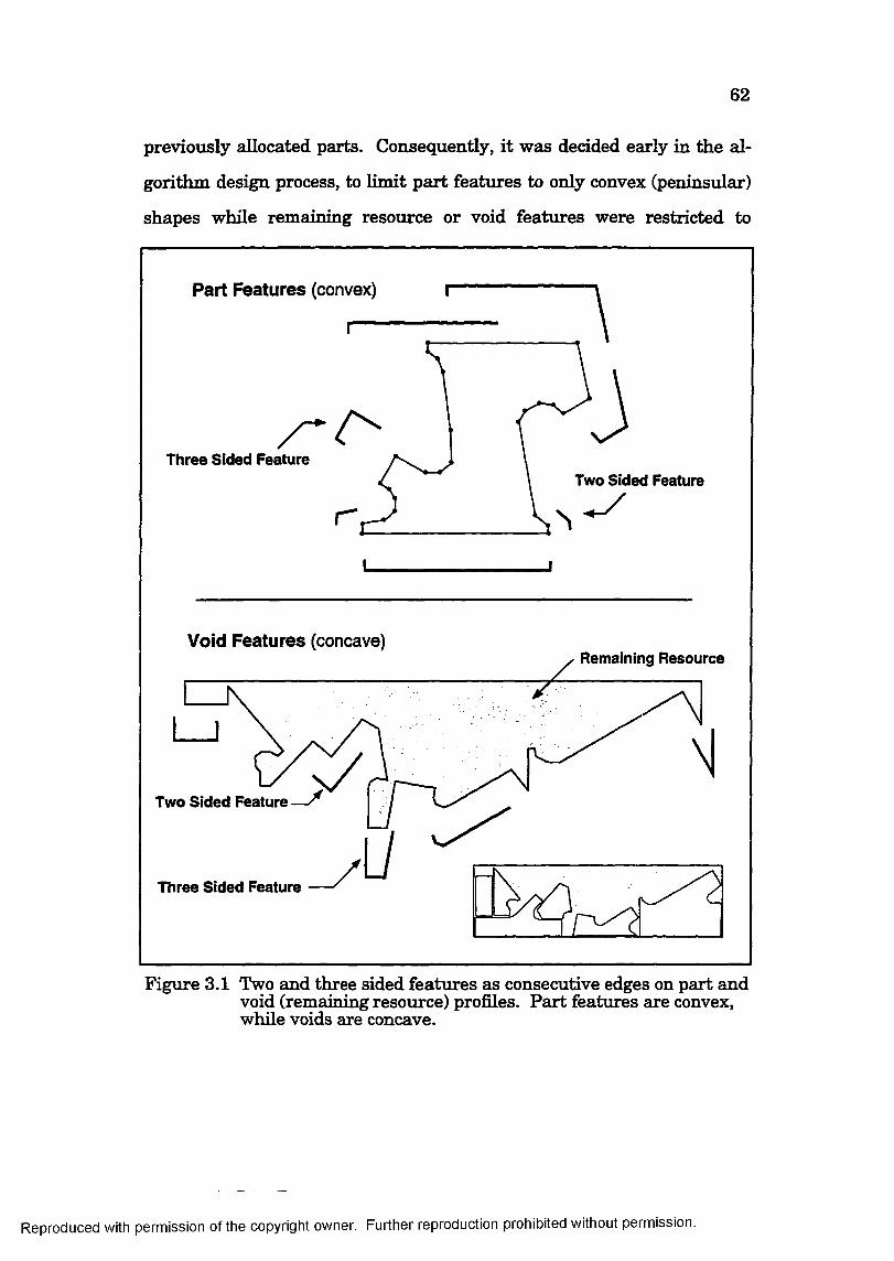
62

previously allocated parts. Consequently, it was decided early in the al

gorithm design process, to limit part features to only convex (peninsular)

shapes while remaining resource or void features were restricted to

Part Features (convex)

Three Sided FeatureTwo Sided Feature

Void Features (concave)Remaining Resource

Two Sided Feature —^

Three Sided Feature

Figure 3.1 Two and three sided features as consecutive edges on part and void (remaining resource) profiles. Part features are convex, while voids are concave.


63

concave notches. Examples of such void and part features are shown in

Figure 3.1.

If restricted to three sequential edges of the actual profile,

the notion of a feature still supplies only a localized characterization of

the shape. The general problem of nesting parts of varying size and com

plexity requires information about shape at various scales. When placing

small parts finer detail is required. However, this additional detail com

plicates the positioning of larger parts and is of little use. This is demon

strated in Figure 3.2. To obtain a more global characterization, simplified

SmallDetailRequired

SmallDetailIgnored

Figure 3.2 The utility of shape characteristics at various levels of detail during p ^ placement.


64

profiles which approximate the original shape at varying levels of detail

are produced. Once such profiles exist, features are easily extracted us

ing straightforward heuristics, which examine each set of three sequen

tial sides and their two included angles. In this way a hierarchical group

of features describing both minuscule and large scale characteristics of a

profile can be constructed.

Part and void profile simplification is accomplished using a

series of techniques detailed in the following sections. The methods for

processing are outlined with respect to the remaining resource first, as

part profiles are handled using a subset of these same methods. The com

bination of these techniques to produce the idealized representations

needed for effective features is then discussed. Finally the nomenclature

and conventions used to define the descriptive information stored with

each feature are presented.

3.3 Profile Sim plification Techniques

Methods of approximating a part profile with varying de

grees of detail have been studied by many [DAVI77], [FAVL74], [PAVL78]

[ROSE73], [ROSE751, [H0R0751, [FREE741. The current method pro

poses to use features for non-overlapping placement, requiring they be ex

tracted from approximations completely inscribing (voids) or circumscib-

ing (parts) the original profile. The need for this restriction will become

evident in Chapter Four. This is the major impediment to implementing

previously reported techniques. Consequently a series of procedures

geared specifically toward the objectives of the allocation problem were

developed. These methods are discussed first with respect to


65

simplification of the remaining resource; the same concepts are also ap

plied to parts.

Simplification of the void is accomplished through two gen

eral techniques. The first, small complexity reduction (SCR), eliminates

inconsequential shallows, ridges, and fillets by examining each profile

vertex and its two adjacent sides. Since the effect of such methods is lo

calized to only a small portion of the profile, the extent of the simplifica

tion is limited. The second technique, large scale resource division

(LSRD), eliminates complexity at a global level, splitting the void a t loca

tions of necking and evaluating the usefiilness of the regions based on

their shape and size. The rem aining resource is simplified when unsuit

able areas are eliminated.

3.3.1 Sm all Complexity Reduction

SCR is divided into three separate routines which eliminate

shallows, ridges and chamfers respectively. Acceptable candidates for

elimination are detected by calculating the height of each vertex of the

void profile. The height of a vertex is the perpendicular distance fi-om the

line connecting its two adjacent vertices. This is given as

Hi = ((EiX Eq^ ) ' u^) ! \Eq^ I [3.1]

where E qj represents the crossing edge and is defined as

^ C R = ^(i+1) ' ^(i-1) . t^.2]

Negative vertex heights represent concave shallows while positive values

represent convex ridges (Figure 3.3). If the magnitude of a vertex height

falls below a set tolerance, SCR_HTOL, a candidate for elimination ex

ists. The value of SCR_HTOL is selected firom experience to be represen

tative of smaller details.


66

i+2 Convex Ridoe H .> 0

1-1

i+1 i-2i-2

i-1Crossing Vector >'CR

i+1i+2

Concave ShallowH ,< o

Figure 3.3 A convex ridge and concave shallow and their associated heights

Both adjacent edges point out

Leading Edge

Both adjacent edges point in

One adjacent edges points in

TrailingEdge O New Vertex

® Eliminated Vertex

• • • New Edge

Figure 3.4 Convex shallow elimination methods


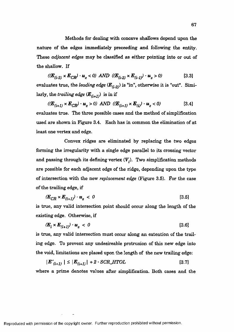
67

Methods for dealing with concave shallows depend upon the

nature of the edges immediately preceeding and following the entity.

These adjacent edges may be classified as either pointing into or out of

the shallow. If

^^(i-2) ^ AND ((E - 2) ^ ^(i-lp "^2^0^ [3.3]evaluates true, the leading edge is "in", otherwise it is "out". Simi

larly, the trailing edge is in if

^^(i+1) ^ " * 2 ^ AND X ’ **2 ^ ^ [3 .4]evaluates true. The three possible cases and the method of simplification

used are shown in Figure 3.4. Each has in common the elimination of at

least one vertex and edge.

Convex ridges are eliminated by replacing the two edges

forming the irregularity with a single edge parallel to its crossing vector

and passing through its defining vertex (Vp. Two simplification methods

are possible for each adjacent edge of the ridge, depending upon the type

of intersection with the new replacement edge (Figure 3.5). For the case

of the trailing edge, if

®Ci2 ^ ^(i+1? ' 0 [3.5]is true, any valid intersection point should occur along the length of the

existing edge. Otherwise, if

^ < 0 [3-6]is true, any valid intersection must occur along an extention of the trail

ing edge. To prevent any undesireable protrusion of this new edge into

the void, limitations are placed upon the length of the new trailing edge:

I I s I I + 2 • S C R jrrO L [3.7]

where a prime denotes values after simplification. Both cases and the


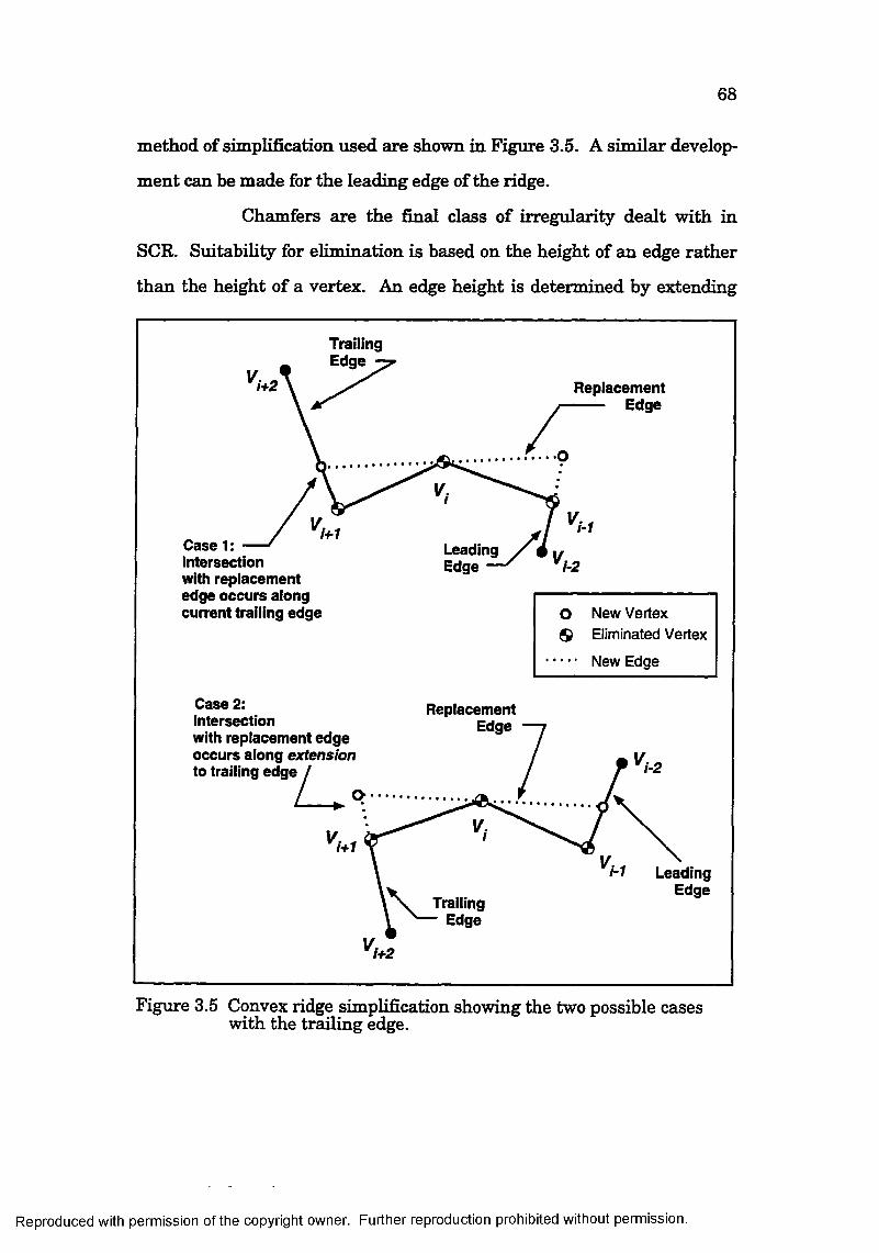
68

method of simplification used are shown in Figure 3.5. A similar develop

ment can be made for the leading edge of the ridge.

Chamfers are the final class of irregularity dealt with in

SCR. Suitability for elimination is based on the height of an edge rather

than the height of a vertex. An edge height is determined by extending

Trailing Edge

Replacement Edge

Case 1 Intersection with replacement edge occurs along current trailing edge

Leading Edge

o New Vertex9 Eliminated Vertex

New Edge

Case 2:Intersection with replacement edge occurs along extension to trailing edge

ReplacementEdge

Trailing Edge

1/i-1 Leading

Edge

Figure 3.5 Convex ridge simplification showing the two possible cases with the trailing edge.


69

the two adjacent edges ^ t i l an intersection is found. The

height of the edge in question is the distance of this intersection from .

Only edges defined by two convex vertices need be examined. If this

height falls below the SCR_HTOL, a comer is extended as shown in Fig

ure 3.6. As with shallow and ridge elimination, all new edges must be

checked for intersection with the current profile.

i+1

i-1

Edge Height

Chamfer Simplification

o New VertexEliminated Vertex

New Edge

i+1

Figure 3.6 Edge heights and chamfer elimination

The elimination methods for each irregularity are imple

mented in three separate routines : SHALLOW_RMV(), RIDGE_RMV(),

and CHAMFER_RMV( ). Although simplification techniques differ, the

underlying structure of each routine is the same. Upon entry, the height

of all acceptable entities for that routine are calculated once and sorted

into ascending order. Irregularities are then removed in sequence from

smallest to largest. To prevent potential conflicts with previously


70

removed adjacent irregularities, all alterations and eliminations of edges

and vertices are recorded. If any substantive changes have occurred to

the profile elements required for the simplification of that entity, it is ig

nored. Processing continues in this way until all of the non conflicting eli

gible irregularities are removed.

3.3.2 Large Scale Resource D ivision

The second method of simplifying the remaining resource is

LSRD. LSRD is achieved through splitting a void into several regions a t

areas where necking occurs. The objective is to m aintain larger useful ar

eas, while eliminating smaller unusable ones where the likelihood of suc

cessful placement of parts is m inim al. Simplification is achieved in multi

ple steps through the decomposition of the void along dividing lines

(DL’s). The method is depicted graphically in Figure 3.7. At each stage

three actions may be taken with each of the available sub-regions.

• DIVIDE Divide the subregion a t its shortest DL.

• ELIM INATE Simplify the remaining resource by completely elimi

nating the subregion.

• ACCEPT End processing of the subregion and incorporate it

into the simplified description of the rem ain ing re

source.

Four criteria determine the action taken with each subregion. Figure 3.8

indicates how these are used.

• AREA True if the area of the subregion is smaller than a set

tolerance (AREAJTOL).

• CONCAVE True if all vertices of the subregion are concave.


71

Permanent Dividing Line Temporary Dividing Line Remaining Resource Profile

I I Useful Area ^ Un-Usabie Area (F.F, ♦, *) Divide

(F,T,T,T) Eliminate(F,F,*,*) Divide

(T,*,T,*) Eliminate

(F.F.*.*) Divide (F.F,*,*) Divide

n

( F . F D i v i d e (T,T,F,*) Acceptr ,

(F.T.F,*) Accept (F,F,*,*) Divide

(T,*,T,*) Eliminate (F.T.F,*) Accept (F,T,T,F) Accept

Figure 3.7 The LSRD process. Quadruples preceding each action represent values of the decision criteria (Area, Concave, Side, MER) for that subregion. Asterisks indicate the criteria is not required to determine the action shown.


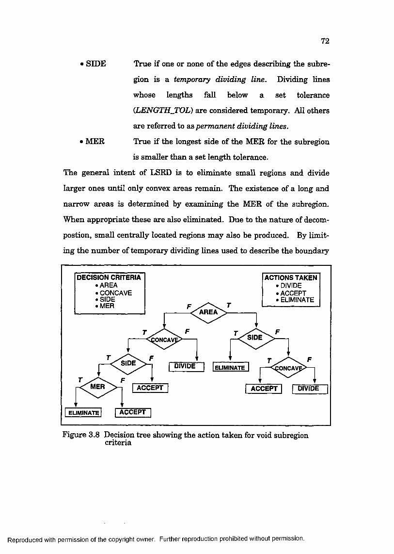
72

• SIDE True if one or none of the edges describing the subre

gion is a temporary dividing line. Dividing lines

whose lengths fall below a set tolerance

{LENGTHjrOL) are considered temporary. All others

are referred to as permanent dividing lines.

• MER True if the longest side of the MER for the subregion

is smaller than a set length tolerance.

The general intent of LSRD is to eliminate small regions and divide

larger ones until only convex areas remain. The existence of a long and

narrow areas is determined by examining the MER of the subregion.

When appropriate these are also eliminated. Due to the nature of decom-

postion, small centrally located regions may also be produced. By limit

ing the number of temporary dividing lines used to describe the boundary

DECISION CRITERIA ACTIONS TAKEN• AREA • DIVIDE• CONCAVE • ACCEPT• SIDE • ELIMINATE• MER p T

------------^^a r e a N -------------

T F

MER

SIDE

F

DIVIDE ELIMINATET F

ACCEPT ACCEPT DIVIDE

ELIMINATE ACCEPT

Figure 3.8 Decision tree showing the action taken for void subregion criteria


73

of the of subregions, their unnecessary elimination is prevented. Exam

ples of each condition can be found in the idealized profile of Figure 3.7.

The degree of simplification produced by LSRD is deter

mined by the values of AREAJTOL and LENGTHJTOL, which in practice

are adjusted to reflect the representative size and dim ension of the set of

remaining parts. To achieve this goal, each profile’s characteristic dimen

sions are represented by the height and width of its MER, while its area

is used to indicate size. Parts previously placed and those larger than the

current resource are eliminated. The distribution of these measures

across the part set is highly variable and unknown [HART851,

[SUMM87]. Consequently, an approximate description is generated by

sorting the remaining values, and tabulating the averages for the small

est, middle and largest third. The three tolerance pairs are generated to

produce the different levels of detail needed for nesting. Results achieved

by varying the two parameters are shown in Figure 3.9. After simplifica

tion what remains are the useful regions suitable for the profiles de

scribed by a tolerance pair.

The LSRD technique is implemented in a routine called

DIVIDE_REGION( ). The algorithm is structured to divide and simplify

the profile it receives until a permanent dividing line is encountered.

When this occurs, processing stops and the two separate subregions pro

duced are returned, along with any simplifications to their profiles accom

plished prior to this division. Otherwise processing continues until no

further simplifications can be made, and the resulting totally reduced pro

file is output. Structuring of this type allows integration with the previ

ously mentioned SCR routines.


74

Merged Profile (305 cm. x 1219 cm.)

AREAJTOL = 2580 cm." LENGTH_TOL = 25 cm.

AREA_TOL = 4516 cm.^ LENGTH_TOL = 51 cm.

AREA_TOL = 9677 cm.^ LENGTH TOL = 102 cm.

Figure 3.9 Different levels of detail produced by varying the area and division tolerances of the void simplification algorithm.


75

3.4 Void Sim plification

The SCR and LSRD techniques are combined, as shown in

Figure 3.10, to produce the profiles firom which void features are ex

tracted. Input to the algorithm is supplied by a queue of profiles, which

CHAMFER_RMV() -4-------------------

WHILE (Proff) CHANGED

SHALLOW_RMV() M-------------------

WHILE (Proff) CHANGED

±RIDGE_RMV()

WHILE (Prof j) CHANGED

D!VIDE_VOID( )2 Sub-Regions

Produced Sub-Prof,

Sub-Prof.

Single Reduced Profile Produced

CHAMFER_RMV( )

WHILE (Prof f) CHANGED

SHALLOW_RMV( ) ----------------------

WHILE (Prof,) CHANGED

RIDGE_RMV( )


Prof,TfoT,Prof,

InputQueueofProfiles

Figure 3.10 The void profile simplification algorithm


76

initially contains only the unsimplified remaining resource. Each profile

is originally processed using the SCR routines. The CHAMFER_RMV( )

routine is used first, and is called repeatedly until no further simplifica

tions can be made. The concave shallow and convex ridge routines follow

in a similar fashion. The resulting profile is then operated on by the DI-

VIDE_VOID( ) algorithm. If two subregions are produced, each is submit

ted to the input queue for further processing. When a single reduced pro

file results, it is subjected to the SCR routines one final time and the out

put stored. Processing continues in this way until the input queue is

emptied. As shown in Figure 3.9 multiple disjoint regions can result.

3.5 Part Sim plification

Unlike the remaining resource, approximations of the part

profiles are produced using only SCR methods. Several arrangements

were investigated, however the combination of routines shown in Figure

3.11 produced the best results over a wide range of shapes. Initially, the

part profile is simplified by executing SHALLOW_RMV( ) repeatedly

until no changes can be made. This is followed by a single run with the

chamfer and ridge removal algorithms. The entire sequence is then re

peated until no unacceptable irregularities remain. Differing levels of de

tail are achieved by varying the maximum allowable irregularity height,

SCR_HTOL. Since this differs depending on the size of the part, the tol

erance is set dynamically as a percentage of the profile's MER diagonal.

For the current application, 15%, 20% and 30% are used to produce pro

files of small, medium, and large detail. Sample results are shown in Fig

ure 3.12.


77

Profile f

SHALLOW_RMV()



CHAMFER_RMV()

Figure 3.11 The part profile simplification algorithm

3.6 F eature Extraction and Storage

To produce a descriptive set of features for a void, its profile

is first approximated at three levels of detail through profile simplifica

tion. A similar procedure is followed for parts, with the MER also added

to the normal collection of approximating profiles. Features are easily de

termined by searching the descriptions generated for the required cove

and peninsula shapes. For voids, a three sided feature coincides with each

pair of adjacent concave vertices, while for parts a pair of convex vertices

is needed. Other useful sections of the remaining resource are detected

by permitting a special two sided void feature. As shown in Figure 3.13,

these areas coincide with a single concave vertex bordered by a convex

vertex on both sides. With this exception, all other part and void features

are three sided.


78

A separate set of features is extracted from each, representa

tion generated through profile simplification. Although these profiles

Original Profile

High Detail

Medium Detail

Low Detail

Figure 3.12 Different levels of detail produced by the part profile simpH-Different levels of detailfication algorithm


79

correspond to different levels of detail, identical features can occur and

are eliminated. Those remaining are then combined to produce a single

set of unique features for each part or void.

Information used for the selection and placement of parts is

stored with each feature. With reference to the remaining resource, this

Two Sided — Feature Three Sided

I— Feature

• Convex Vertex o Concave Vertex

IV'IV

’2V3V 'FeatV

■2V

’B V

Figure 3.13 Information stored with each feature


80

includes the length of each side ( Zjy, ), and the two included

angles (0 jy , 8gy). Numerical labeling indicates the order of appearance

in the clockwise oriented void profile. The angle between sides one and

three of the feature is calculated (8gy), giving an indication of the "open"

(8gy > 0) or "closed" (8gy > O') nature of the profile segment (Figure 3.13).

The void feature's position with respect to the original (unsimplified) re

maining resource is maintained by storing its constituent vertices (

V^y, V^y, V^y) OS meusured in the stock plates local coordinate system.

Vertices 2 and 3 are referred to as interior, while 1 and 4 are exterior.

The feature orientation is specified by the angle between the hori

zontal and the middle, center, or second side (VgVg) of the feature. Two

sided features are treated as a special case of the three sided variety, with

either I jy and 8jy, or Igy and 8gy set to zero, and 8gy left undefined.

Similar information is stored with each part feature using

the same notation and a subscript "P"; however, the part’s local coordi

nate system is used. Although part profiles are oriented counterclock

wise, their feature information is labeled in a clockwise fashion for consis

tency when doing void feature comparisons.

With features constructed and stored, the basic information

required for a shape reasoning solution is available. As will be shown in

the next chapter, this information can be exploited to both generate and

select candidate part placements.


C hapter Four N estin g w ith Features4.1 Introduction

Building layouts through the sequential addition of parts to

a resource involves two primary tasks, part selection and part placement.

Each stage of the solution requires that a choice be made fi-om the infinite

number of locations and orientations possible for each of the unplaced

parts. The geometric information of the part and void features is ex

ploited to reduce the options fiom an infinite number to a workable set.

The use of features for the selection and placement of parts

is detailed in this chapter. Although selection would seem to logically

precede placement, in practice the decision strategies for both are inter

twined. Several precepts are common to both processes and are best un

derstood in the context of part placement. With this in mind, placement

is detailed first.

4.2 Part Placem ent

Placement of a part onto the resource requires establishing

both its orientation (0) and location (x,y). By "matching" complementary

void and part features key information is provided for determining both.

Positioning is achieved through a series of steps, with a part

orientation selected first. A desirable value is picked fiom those rotations

aligning the sides of the paired part and void feature. The part orienta

tion is then held fixed and its best location found.

The initial part position is establish by determining the way

in which the two involved features mesh or fit together. Each of the

81


82

different possible fits is referred to as an align type, and criteria deter

mining the existing case may be derived. The objective of these arrange

ments is to provide an initial non-overlapping placement of the part

which is immediately adjacent to a complementary void shape. Since

features are only an approximate representation of the actual void and

part profiles, the placement indicated by the align type is only an initial

estimate. If the part falls totally within the void, then its position is

further refined by shifting along the true void boundary until a final

placement is found. Each of these steps is detailed fiirther in the follow

ing sections.

4.2.1 O rientation

Potential part orientations are derived by matching features.

For a given pair, the developed method supplies three orientations corre

sponding to alignment of each part feature side with its complement on

the void (Figure 4.1). For alignment of side two of the part feature with

side two of the void feature, the required rotation of the part is

given as

^ R O T F e a t V ' ^ F e a t P . ^4.1]

Similarly, for side one ahgnment the rotation angle is

^ROT - ^FeatV ' ' ^FeatP + ®2P , 1 4.2]

and for side three

Qr Ot = ^FeatV + ' ^FeatP '

The aligned edges in each case are referred to as the primary sides of the

match.

Part rotations for matches between two sided void features

and three sided part features are also provided through side alignment.


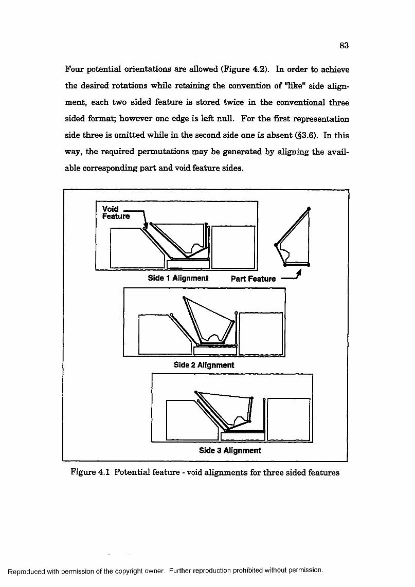
83

Four potential orientations are allowed (Figure 4.2). In order to achieve

the desired rotations while retaining the convention of "like" side align

ment, each two sided feature is stored twice in the conventional three

sided format; however one edge is left null. For the first representation

side three is omitted while in the second side one is absent (§3.6). In this

way, the required permutations may be generated by aligning the avail

able corresponding part and void feature sides.

Void _ Feature

_ /Side 1 Aiignment Part Feature

Side 2 Aiignment

Side 3 Alignment

Figure 4.1 Potential feature - void alignments for three sided features


84

‘2V

Part Feature

’’3V

1st Void Feature Representation

Side 1 Alignment

Side 2 Alignment

2nd Void Feature Representation

Side 2 Alignment

Side 3 Alignment

Figure 4.2 The four orientations provided for 2 sided void features

4.2.2 Align Types

Once the primary side of a match is selected, an align type or

the way in which the two features mesh or fit together is established.

Figure 4.3 shows a few of the many align types possible for each of the

primary side alignments. A complete list of all supported types is pro

vided in the Appendix A.I. Resolution of the align type determines the


85

relative location of the part feature with respect to its void complement.

Since part orientation and the location of each feature with respect

to the entity it describes are known, finding the relative positioning of the

two provides the remaining information necessary to initially place a part

(x,y).

Align Side 1 Aiign Side 2 Align Side 3

Type IB Type 21 Type 3J

Type II Type 2A Type3E

• Void Feature » Part Feature

Figure 4.3 Different fits or align types possible between two features

The arrangement of each align type is chosen such that the

part feature is shifted as far as possible into the void feature. The objec

tive of such positioning is to provide an initial placement of the part to

tally contained within the rem aining resource and adjacent to a comple

mentary shape. These align type positions are characterized by finding a

point of contact between the void and part features. Different interac

tions may occur, but all can be represented as either a part feature vertex

falling upon a void feature side, or a void feature vertex falling upon a

part feature side. Regardless of which case exists, these intersecting enti

ties are referred to as the align type reference vertex and the align type


86

reference edge, respectively. The location of the reference vertex upon the

reference edge is designated as the a l i ^ type reference distance

The correct elements for each align type are listed in Tables A.1 through

A.3.

For any match of two features, a series of calculations can be

performed to determine their relative positions. Although each match is

unique, commonalties between cases can be exploited to simplify the pro

cedure. Each align type represents a group of matches having the same

conditions for existence. In all cases these criteria can be expressed as a

system of linear equations and a set of inequalities constructed from the

feature data itself. Satisfaction of the criteria also determines the rela

tive position of the features themselves. This information is catalogued

for all supported types. Thus, the arrangement of a particular match may

be determined by comparisons to the required criteria stored for each

align type.

The set of supported align types are further organized into

two large groups or classes, based on similarities in their existence crite

ria. The touching class contains all cases where one or both interior ver

tices of the part feature contact the center edge of the void feature. The

second non-touching class contains all others. Physical similarities be

tween all matches in a class permit the analogous formulation of the in

equalities and equations needed for their existence. An example from

each class is described below. The defining criteria for all other align

types within each class may be derived using similar reasoning.

Align type 2C (Figure 4.4) represents the most general case

of the touching class. Shifting along the primary sides is possible once


87

the part feature has been translated its farthest extent into the void.

This extra degree of freedom is eliminated by shifring side two of the part

feature as far as possible toward one of the non aligned sides of the void.

The direction chosen is based on the absolute difference between the cor

responding angles of the two features. If

1 V - îp I < 102V ■ ®2P I [4.4]

is true, shifting is toward I^y, otherwise it is toward Zgy . The edge se

lected is designated the secondary side of the match, as it is the edge most

closely associated with the primary sides. Although variable when align

ing the middle side of two features, for alignment of sides one or three it

is always side two.

Regardless of the side chosen as secondary, the farthest ex

tent which the part may be moved in either direction must be calculated

to determine if type 2C exists. With reference to side one, two cases may

occur. The first edge of the part feature may be either "in" or "out" of the

void (Figure 4.4). Using the triangle formed by Zgy, and Z p , it can be

shown that if

Zjp* sin(Q2 p) Z sin(Q2 '} ^ 2V [4.5]

is true, Zjp is "in" and the location of the reference vertex (Vjp ) along the

reference edge is given as

^ÂT^siDE 1 ~ sin(Q2p ~ 0jy) " Zjp / sin(Q2y) • [4.6]

Otherwise side one is "out" and

^ÂT^siDE 1 ~ sin(Q2p * 0jy^ * Z^y / sZn(8jp) . [4.7]

A similar formulation can be made for side 3. Case 20 exists if

( ( s j ^ j ‘) s n 3 E i + ^â t ^ s i d e s ^ ^ 2 V • [4 .8]


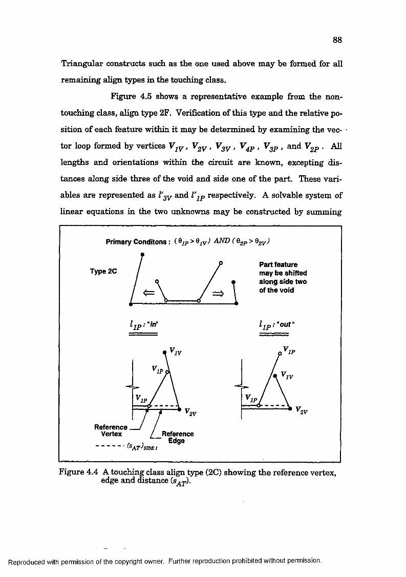
88

Triangular constructs such as the one used above may be formed for all

remaining align types in the touching class.

Figure 4.5 shows a representative example from the non

touching class, align type 2F. Verification of this type and the relative po

sition of each feature within it may be determined by examining the vec

tor loop formed by vertices V j y , , V ^ y , V^p , V^p , and • All

lengths and orientations within the circuit are known, excepting dis

tances along side three of the void and side one of the part. These vari

ables are represented as I'^y and respectively. A solvable system of

linear equations in the two unknowns may be constructed by summing

Primary Conditons : ( ip > ^ly) AND ( 8^^ > 8gy^

Part feature may be shifted aiong side two of the void

Type 2C

IP-

IPIV

IV

IPIP

2V2V

ReferenceVertex Reference

Edge

Figure 4.4 A touching class align type (2C) showing the reference vertex.Aedge and distance (s./r)


89

distances around the loop in the horizontal and vertical directions. The

following result is derived.

^2V~ ^1V‘ ^3P‘ - ^2P— 13V* cos(6g^ - 12 p ' cos(Q2 p) [4.9]

l^p' sin(Q2p) - I jv' sin^Qpy)— 13v' " / 2p' siîi(Q2p) [4.10]

Using these equations, the values of I'^y and I'jp may be calculated. The

following metric is then used to verify the type. If

(0<l '3y<l3y) AND (0<r2p<lgp) [4.11]

then type 2F exists. The relative location of the part is provided by set

ting equal to I ' ^y .

All non-touching align fypes contain a vector loop which may

be formulated in terms of two unknown edge lengths. By constructing the

necessary loop equations for each arrangement in advance, a simple and

quick method for determining align type is available for all arrangements

in this class.

Primary Conditons : ( Gjp > Q^v AM? ( 6gp >

IP2V

4P

IPAlign Type 2F IV3P 2P

Figure 4.5 Non-touching class align type 2F


90

4.2.3 In itia l Placem ent and Shifting

Using the information provided by the align type and pri

mary sides, an initial placement of the part onto the resource may be gen

erated. This placement is only an estimate of the part’s finsil location

however, as the void and part features used for its generation are only ap

proximate representations of the actual profiles involved. A final place

ment is produced by sliding the part along the actual boundary of the re

maining resource using the INFP technique discussed in chapter 2. To

guarantee construction of the INFP, the initial placement must be valid

(i.e. the part must be totally contained within the void). Conversely, an

invalid initial placement occurs when any portion of the part profile falls

outside of the remaining resource, usually at some distance away firom

the features.

An initial position is verified by checking for possible inter

sections between the two profiles involved. The computational expense

for this is substantially reduced by first applying a Cyrus-Beck clipping

algorithm to eliminate those void edges falling outside an approximate

boundary enclosing the part [HILL90]. The convex clipping window re

quired for this technique is provided in most cases by the simplified pro

files used during part feature extraction. Otherwise a part’s MER is

used. All void edges not eliminated must be checked for possible intersec

tions with the part using conventional methods.

All valid initial placements are further refined by shifting

the part as far as possible in an allowable shift direction derived firom the

part orientation and the angles of the void feature involved. Figure 4.6

shows the three possible cases. For side one alignment, a shift direction


91

toward the remaining resource is constructed by bisecting Bisection

of 8gy and Q^y are used for alignment of the third and center sides, re

spectively. The part is translated in this direction until it contacts the

void boundary. The contact vertices needed to initiate the INFP may

then be found. The part is moved along the void boundary in either a

clockwise or counter clockwise manner dependent upon which is consis

tent with the desired shift direction.

The IN FP proceeds in a fashion sim ilar to tha t described in

Chapter Two; however, its construction over the entire remaining

Align Side 1 Align Side 3 Align Side 2

Bisect 8Bisect 8Bisect &2V BV2V

Shift Direction

Figure 4.6 The three possible shift directions determined by the void fea-shift directions determinedture angles and the aligned sides of the match.


92

resource boundary is not required. As before, movement vectors (§2.2.1)

are provided by the edges of the void and part profiles. Shifting along the

remaining resource boundary is permitted until a translation which op

poses the allowable shift direction is detected by

S - S ^ < 0 , [4.12]

being true, where S is a movement vector and is the allowable shifi;

direction described above. When this occurs, construction of the INFP is

halted and the current part’s position set as its final placement.

Two additional restrictions are also imposed during the part

placement procedures. The first pertains to the amount of movement oc

curring between the initial to final placements. During INFP shifting, it

is possible for the part to migrate beyond the region of the resource in

tended (Figure 4.7). In these cases, the benefit of matching the comple

mentary shapes of the void and part features is often lost. These in

stances are detected and eliminated by limiting the total shift distance

permitted to a pre-set percentage of the length of the part’s MER.

The second restriction pertains to the allowable shift direc

tion used in placement. A natural affinity exists for part placements

along the long straight edges and square comers of the square resource

stock due to the complementary shape reasoning heuristics implemented.

Experience shows that this bias causes layout generation to proceed unfa-

vorablely inward firom the outer boundaries of the plate. To overcome

this tendency, restraints are placed on the use of those border features

containing elements coincident with the boundary of the original stock

material.


93

Void Feature —

Initial Placement

ShiftDirection

Final Placement

Part Feature

Figure 4.7 An example of the placement procedure where a part shifts beyond the intended region characterized by the void feature.

When such a border feature is involved, the allowable shift

direction must fall between two limits, otherwise the match is ignored.

These limits are referred to as the border feature shift directions and are

defined by two angles measured firom the horizontal, Qsmin Qsjîax •

For example, parts will favor the upper left hand comer of a rectangular

resource, when border feature shift directions are set between 90“ and

180“. In such an arrangement, placements proceed firom the left


94

downward in a more bene&dal manner. Additional control is also ob

tained by varying the acceptable shift direction range between part place

ments. The characteristics of the solution can be changed considerably

using the border feature shift directions as will be shown in the next

chapter.

To summarize, four steps are involved in placing a part (Fig

ure 4.8).

1) Choose a primary side to orient the part with respect to the

resource.

2) Determine the the align type for the selected features.

3) Locate the part using the align type and determine if it falls

totally within the rem aining resource.

4) Shift the part as far as possible within the void in the direc

tion specified by the aligned sides.

4.3 Part Selection

As indicated above, given a matched pair of features it is

possible to determine if a valid part placement or match exists. In prac

tice, it is not unusual for each part to have five to ten features while the

remaining resource may have more than twenty. The high volume of com

binations makes it impractical and expensive to examine all possible part

and void feature pairings. As a consequence a quick and computationally

efficient method for determ ining the quality of the match between two

features is needed. The strategy used is to calculate a single number

measure or matching index for each possible a lignm en t of a pair. The nu

merous matches can then be prioritized, and evaluations limited to those

selected as best.


95

The matching index for a pair is evaluated using three basic

geometric difference measures between the part and void features

involved. These measures are calculated separately using the information

stored with each feature, and are then combined to produce the single

matching index. Since complementary shapes are sought, smaller differ

ences are considered favorable. Consequently, the index is formulated

such tha t lower values indicate a better match.

The first diiBference calculated is that between the primary

angles of the match. The primary angle of each feature is included be

tween its primary and secondary sides. The measure is calculated as:

- 0 /(Primary V) (Primary P) [4,13]

Step 1

Void Feature Steps 2 & 3

Primary Side

Primary Side

Align Type & Initial Placement

Part Feature

Step 4

Shift Direction

Shifting for Final Placement

Figure 4,8 The four steps of part placement: 1) Select features and orient part, 2) Determine align type, 3) Initial placement, 4) Part shifting.


96

This difference is considered the most significant indicator of a good

match since it corresponds to the angle between the void and part secon

dary sides (Figure 4.9). The value of P must fall below a tolerance (P-joL »

otherwise no index is produced and the match discarded. The role of

matching index tolerances is discussed more fully in Chapter Five; how

ever, the general intent is to eliminate the unnecessary calculation of un

favorable indices.

Primary Side 1

Secondary Sides

Primary Side 2 Primary Side 3

Secondary SidesSecondary Sides — ^

Figure 4.9 Angle P, the difference between the primary angles of a match for the three primary side alignments

If the calculated value of P is acceptable, the align type of the

feature pair is determined. Only touching class align types are currently

accepted, based on the premise that these types are the most likely to pro

duce valid initial part placements. The arrangement of individual feature

elements within the align types of this class also allow the straightfor

ward calculation of meaningful difference measures. Similarities across

the class can be exploited in the formulation of the matching index, per

mitting more consistent comparisons between the different align types. If

the ahgn type is accepted, its positioning information is stored and used

for the calculation of the next difference measure.


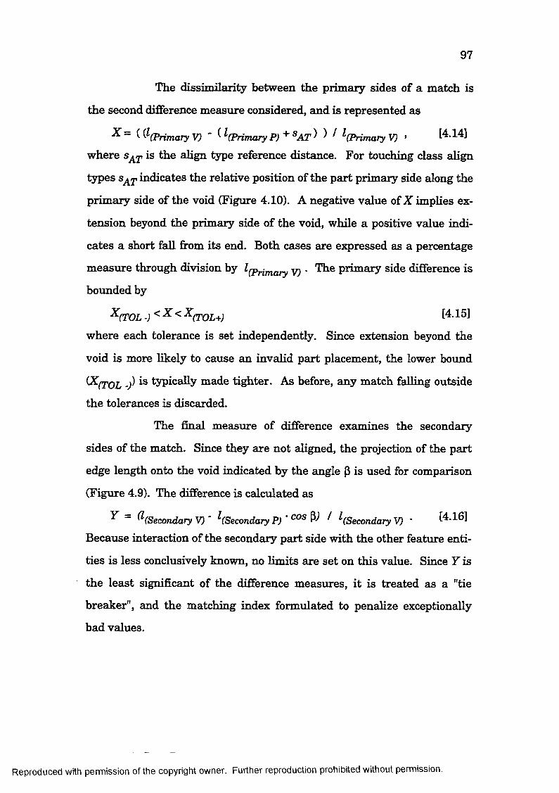
97

The dissimilarity between the primary sides of a match is

the second difference measure considered, and is represented as

^ - ( ^^(Pnmary V) ' ( ^(PHmary P)'^^AT^ ) ^(Primary V) > where is the align type reference distance. For touching class align

types indicates the relative position of the part primary side along the

primaiy side of the void (Figure 4,10). A negative value of X implies ex

tension beyond the primary side of the void, while a positive value indi

cates a short fall from its end. Both cases are expressed as a percentage

measure through division by l(primary V) ' primary side difference is

bounded by

^(TOL < ^(TOL+)

where each tolerance is set independently. Since extension beyond the

void is more likely to cause an invalid part placement, the lower bound

(X(tol typically made tighter. As before, any match falling outside

the tolerances is discarded.

The final measure of difference examines the secondary

sides of the match. Since they are not aligned, the projection of the part

edge length onto the void indicated by the angle P is used for comparison

(Figure 4.9). The difference is calculated as

Y — (^(Secondary V) ~ ^(Secondary P) ’ ^(Secondary V) ' [4.16]Because interaction of the secondary part side with the other feature enti

ties is less conclusively known, no limits are set on this value. Since Y is

the least significant of the difference measures, it is treated as a "tie

breaker", and the matching index formulated to penalize exceptionally

bad values.


98

The three raw difference measures are incorporated to form

a single matching index. Recalling tha t a smaller index should indicate a

better match, the measures are combined as follows.

MATCHINDEX (. [4.17]I TOL \^TOL-hJ " \^T O lJ

Within the formula, P and X are each normalized using their respective

maximum limits. Since X is considered a less significant measure, its in

fluence on the matching index is reduced by squaring its normalized

value. The secondary side measure is also adjusted through division with

YtoL’ ^ desired hmit set for that variable. Any Y values falling outside of

the tolerance are automatically penalized when its adjusted value is

squared ÇYIYj ,qj > 1). Otherwise squaring lessens the effect of this term,

as with X. The final change to Y s significance is made through a weight

ing factor of 0.2. In this way each difference measure is assigned its

proper importance within the matching index.

X > 0

Primary Sides —

'AT

X < 0

Primary - Sides

^AT. o \

Figure 4.10 The positive and negative cases of the primary side measure of difference.


99

Through the use of matching indices, the relative value of all

possible feature combinations can be quickly established. Part placement

techniques can then be exercised to validate any selected match. The two

basic tools for creating a layouts are now available. In the next chapter,

these techniques are integrated with those for feature generation, to pro

duce a comprehensive solution methodology to the bin packing problem.


C hapter 5 Im plem entation and R esu lts5.1 Introduction

In the first half of this chapter the overall solution strategy

for nesting a complete set of parts is presented. The fundamental steps of

the layout generation algorithm are outlined, demonstrating the integra

tion of the feature generation, part placement, and part selection tech

niques previously detailed. The techniques are then combined to produce

a comprehensive search algorithm which generates solutions through the

iterative placement of parts onto a resource. Procedures for dynamically

setting matching index tolerances, and the formulation of a waste fimc-

tion are then discussed. These two additional heuristics are required for

the practical implementation of the solution technique.

In the remainder of the chapter results for a set of industry

supplied part profiles are presented. A group of problems with diverse

characteristics was selected to demonstrate the nature of the solution for

various inputs. The resulting layouts are used to illustrate the robust

ness of the technique. By varying values, the influence of two key input

parameters was also investigated. A series of layouts was generated and

each parameter’s effect upon the performance of the algorithm studied.

Finally, the overall results for the feature based method were compared

with those of the INFP technique used in the pilot study.

5.2 Search Algorithm

Figure 5.1 shows a flow diagram of the primary steps in

volved in generating solution layouts. Part profiles are first

100


101

NoIntermediate Solutions ?

Yes

GenerateSolution

Select a Resource Material

Pre-Process Parts Extract Part Features

Simplify Remaining Resource Extract Void Features

Select Placement with Smallest Waste

Calculate Matching Indices Sort Matches by Index

Generate Intermediate Solutions for First N_SUCCESSOR Successful placements

Figure 5.1 Flow diagram of the primary steps in feature based nesting

pre-processed. At this stage, curves are replaced with piecewise linear

approximations, and if necessary for manufacturing, profiles are offset to

maintain a specified distance between parts on the final layout. The pri

mary role of preprocessing however, is to extract the features represent

ing the parts a t varying levels of detail. This extraction of part features is


102

performed only once as their properties are invariant over the course of

the solution. The geometric information associated with each feature is

stored in a data base which is accessed repeatedly during processing.

Following preprocessing, the stock material for the layout is

selected. The algorithm then advances into the main decision loop where

the majority of work is preformed. Each iteration of this loop represents

the addition of one part to the final solution.

The first step in placing the next part is the simplification of

the resource remaining fi*om the previous stage. Initially, this resource is

the entire stock material. To achieve the appropriate degree of simplifica

tion, a new set of LENGTH_TOL and AREA_TOL values are first calcu

lated based on those parts still eligible for placement. Recalling that

three tolerance pairs representing the smallest, middle and largest parts

are used (§3.3.2), the SCR and LSRD techniques are applied to produce

simplifications of the remaining resource a t varying levels of detail. The

current void features are then extracted and stored.

Matching indices for all possible feature combinations are

now generated firom the part and void data base. Progressing firom most

to least favorable indices, the placements indicated by each pairwise

match are examined and invalid placements due to overlap eliminated.

Each valid placement is called a successor of the current solution, and its

associated part orientation and location are saved. Matches are tested

until a preset number of successors (NJSUCCESSOR) are generated for

the intermediate solution. However, only one is used for further

expansion. Selection of this most favorable placement is based on the

waste function described in the next section.


103

Solution layouts are constructed through the repeated appli

cation of the three primary steps: void feature extraction, matching index

calculation, and part placement generation. Each intermediate stage is

initiated using the remaining resource of the most recently chosen succes

sor. If no successors exist, additional parts cannot be placed on the re

source. The current solution is then output and nesting started on a new

stock blank. The complete solution is realized when all parts have been

allocated.

5.3 W aste Function

At each intermediate stage of the solution a single successor

must be chosen for further expansion. The relative value of each part

placement is distinguished by calculating a waste function for each of the

successors generated. Allocations with smaller waste values are consid

ered more favorable. The appraisal of quality is based on two terms as

sessing the current waste and predicting the future waste of a solution.

Future waste is an estimate of the penalty incurred by allocating all re

maining parts, while current waste deals with the actual trim loss on the

existing layout. This distinction is similar to th a t made by Albano and

Sappupo, however, more intelligent heuristics are used to calculate each

term [ALBA80].

Future waste is calculated as a set percentage of the concave

and true (i.e. actual) areas of all unplaced parts. Each part’s concave area

is defined as the region between its exact and convex hull profile. For the

current application the individual future waste of a part is calculated as

(FUTURE WASTE)^ = 1.0-(True Area)^ + OA-(Concave Area) - . [5.1]


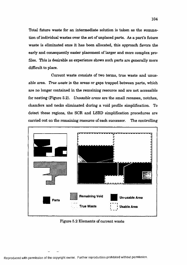
104

Total future waste for an intermediate solution is taken as the summa

tion of individual wastes over the set of unplaced parts. As a part’s future

waste is eliminated once it has been allocated, this approach favors the

early and consequently easier placement of larger and more complex pro

files. This is desirable as experience shows such parts are generally more

difficult to place.

Current waste consists of two terms, true waste and unus

able area. True waste is the areas or gaps trapped between parts, which

are no longer contained in the remaining resource and are not accessible

for nesting (Figure 5.2). Unusable areas are the small recesses, notches,

chamfers and necks eliminated during a void profile simplification. To

detect these regions, the SCR and LSRD simplification procedures are

carried out on the remaining resource of each successor. The controlling

n

PartsRemaining Void

True Waste

Un-usabie Area

J I Usable Area

Figure 5.2 Elements of current waste


105

LENGTH_TOL and AREA_TOL parameter pair required is calculated us

ing only the smallest third of remaining parts. This pohcy prevents the

unnecessary inclusion of waste from areas possibly usable by smaller

parts. Although technically contained within the remaining resource, un

usable area is considered inaccessible based on the size and shape of the

unplaced parts. The regions remaining after simplification are referred to

as usable areas.

The distinction between good and bad placements is often

unclear when based solely upon future waste, true waste, and unusable

area. For example. Figure 5.3 demonstrates two placements of varying

quality which generate equal waste measures. For this reason a perime

ter penalty is calculated to provide additional information for each

successor. Although this term is used to scale the unusable area, it is

e = 1 . 1 9 8 = 1.06

(A)

Un-Usable Area

(B)

Useful Area

Figure 5.3 Two placements of the same part generating equal amounts of un-usable and useful area. Case A has the higher perimeter penalty.


106

calculated by examining the size and shape of usable subregions produced

duing remaining resource simplification. The formulation is:

2-.TCA.)e =[5.2]

where

P- Perimeter of the ijk Usable Area,

A,- Area of the ijb. Usable Area,

^(x) Returns Perimeter of Square of Area x.

All summations are taken over the set of usable subregions.

The two ratios in the denominator are the key elements of

Equation 5.2. The first ratio, $(A^/P^ , is used to measure the "square

ness" of each individual subregion by comparing its perimeter to that of a

square of equal area. Each of these ratios is then weighted based on the

corresponding subregion’s area. By contrast, the second ratio,

^(IAf)/I.(Pj), examines the summation of all subregion perimeters. This

sum is compared to the perimeter of a single square equaling the area of

the combined usable regions. The remaining terms in this metric are

used to scale the penalty such that a value of unity is achieved for the op

timal case. The overall effect of this formulation is to favor a single rec

tangular region over several small irregular ones. Incorporating all

terms, the total waste is calculated as:

TOTAL WASTE = FUTURE WASTE

+ 1.5 • (TRUE WASTE)

+ e • {UN-USABLE AREA) . [5.3]


107

5.4 M atching Index Tolerances

During the solution process, the total number of potential

matches between part and void features can be very large. For sizable

problems, sets of five hundred or more part features and twenty or more

void features are common. Also recall that for each pair of void and part

features, there are three matches corresponding to the three allowed edge

orientations. Such a situation would require the calculation and storage

of thirty thousand matching indices. Since the majority of these repre

sent invalid placements and only a limited number of successors are pro

duced a t each stage of the solution, substantially fewer matching indices

need to be calculated. This is accomplished through matching index toler-

ancing.

A large portion of potential combinations are eliminated by

limiting the values of the difference measures P and X used to calculate

the matching index. As described earlier (§4.3) these value are restricted

as

P < ^crODi [5.4]

and

^(TOL-)i < ^ < ^(TOL+)i » [5-5]

where the subscript i refers to a tolerance level dynamically set through

out the solution. Table 5.1 shows the range of values available for the

current application including those for the parameter (Equation

4.17). For the initial allocation of each resource, tolerances are set to

their most restrictive values, as the pool of available part features is gen

erally large. After each stage of the solution, the number of successors

generated is examined. If the desired number was produced, the


108

tolerances are tightened while remaining in the range of tabulated val

ues. Otherwise they are relaxed to provide a larger pool of potential

matches.

If no vaHd placements can be produced from the set of gener

ated indices, all restrictions on matches are relaxed, and a new set of

matching indices calculated and investigated. This includes all matching

index tolerance values and any potential restriction imposed by the bor

der feature shift directions (§4.2.3). This insures that all possible place

ments are tested and sometimes permits additional allocations.

MoreRestrictive

1Less

Restrictive

Table 5.1 Matching Index Tolerance Values

ToleranceLevel

i ^CTODi ^(TOL+)i ^(TOL-)i ^croD i

1 0.1 0.80 -0.10 0.20

2 0.2 0.90 -0.15 0.40

3 0.4 0.95 -0.20 0.60

5.5 R esults

The shape reasoning methodology introduced has been im

plemented and tested extensively. All algorithms were coded in the C

programming language, and the application run on a VAX 4000-300

server under the VMS operating system. With the exception of input and

output file specification, the package is totally automated.

An industrial marine fabricator provided a diverse set of 42

actual problems to evaluate the robustness of the approach. Each prob

lem included a data file defining the geometry of all unique or master


109

parts and a list of their instances. Part descriptions consisted of straight

lines and circular segments which were approximated with the appropri

ate inscribed (voids) or circumscribed (parts) chords. To reduce the com

putational expense of all profile operations, each part was simplified us

ing the modified convex hull approach of the pilot study [LAM096] and

also offset a prescribed amount to account for flame-cutting fabrication.

Although original part boundaries are plotted in the solution layouts, only

these more practical approximate offset representations are used during

processing.

During preprocessing, the internal voids of larger parts are

extracted and ordered in decreasing size for possible use as irregular re

sources. These regions are nested first. All profiles rem aining are then

allocated to stock standard rectangular plates selected successively fi*om

a prioritized list of available materials provided for each problem by in

dustry. The voids and any associated nests are then re-inserted onto

their parent parts when generating output files.

To help quantify the characteristics of the individual prob

lems investigated, a series of criteria were developed. In addition to total

part count and number of masters, four measures describing the profiles

contained in the problem were defined. Illustrated graphically in Figure

5.4, these are:

Normalized Area =

Irregularity =

Concavity =

Area of Part Profile Area of Stock Resource

Area of Part MER Area of Part Profile

Area of Part Convex Hull Area of Part Profile


110

Complexity = Number of vertices in profile description

Normalized area gauges tiie size of a part relative to the selected re

source. Irregularity measures the non-rectangularity of a profile

[BRON83], while concavity indicates the degree of divergence firom its

convex hull. Complexity refers to the number of vertices in the simplified

profile used for processing.

Irregularity Concavity Complexity

1.00 1.00 4

1.40 1.00 4

1.51 1.36 5

Figure 5.4 Examples of the measures used to describe each part profile

For brevity, mean values of these measures for an entire pro

file set are usually presented. However, averages are sometimes not rep

resentative of the problem nature, particularly when distributions across

the part set are non-uniform. If prompted, the application will furnish a

more detailed problem description, including histograms to demonstrate

the precise distribution of profile characteristics. Additional information

pertaining to aspect ratios and part duplications are also provided. A

problem description of this type is displayed in Appendix A.2.


I l l

5.5.1 Param eter Study

The integral parameters and tolerances of the various tech

niques described throughout this document are the sole method for con

trolling the algorithm performance. When possible, these values are cal

culated by the application, and are allowed to change dynamically during

processing, while others are static and input at run time. In some re

spects, the method is very sensitive to these inputs. A change in parame

ter values may cause the placement of an initial part on a plate to alter

only slightly. This relatively minor change will cascade throughout all of

the remaining steps, making solutions for the same problem set often ap

pear totally unrelated. However, when examining results for an entire

set of problems, small changes do not substantially affect overall waste

and CPU times.

The parameter values currently used are those selected from

experience to produce good overall results for a broad range of problems.

Reasonable ranges for most parameters can be determined in a relatively,

short time through comparative runs of the program.

Two key parameters were selected to demonstrate the na

ture of the solution and the influence of input on the performance of the

algorithm. Two values for the number of successors and the range of bor

der feature shift directions were chosen. Several runs of the application

were conducted to investigate the four possible permutations. The two

cases for shift direction correspond to a constant range of 180“ to 360“ and

a case alternating between the ranges of 90“ to 180“ and 180“ to 270“.

The number of successors was set to 10 and 20. Experience has shown

these values produce reasonable results for rectangular resources.


112

To reduce the CPU time and analysis overhead, a meaning-

fiil and manageable subset of the original 42 industry problems was used

to conduct the parameter study. A heterogeneous group of profile sets

was selected to portray the full diversity associated with the bin packing

class of problem. Table 5.2 shows the characteristics of these problems.

Tables 5.3 and 5.4 summarize the results firom the four cases, including

total CPU time and the number of stock plates used.

For the majority of problems, cumulative waste is identical

in each of the four cases, since nesting the total part set requires the

same number of stock plates. A better indication of quality is obtained by

examining the percent usage for the last plate. A lower value here indi

cates fewer profiles on the final plate, implying better initial packing.

Also, more material remains for nesting of additional parts should they

Table 5.2 Problem set overall characteristics

Prob.Set

Numberof

Parts

Numberof

Masters

AvengeNormaltzed

A naxlOO

TotalNonnalbed

A naxlOO

AverageIrregularity

AverageConcavity

AverageComplexity

StockHeight(cm)

StockWidth(cm)

A 70 50 7.55 528 1.33 1.00 12.2 307 1280B 109 70 19.48 2124 1.15 1.00 11.0 307 1402C 206 70 1.84 378 1.18 1.00 6.6 183 914D 103 60 3.57 368 1.40 1.11 8.3 305 1219E 295 197 2.41 711 1.05 1.03 6.0 305 1219F 52 31 5.05 263 1.21 1.12 6.6 305 1219G 84 49 2.95 247 1.00 1.00 5.5 305 1219H 56 35 6.37 357 1.39 1.18 12.1 305 12191 107 57 6.65 711 1.25 1.08 8.3 305 1219J 111 50 5.21 578 1.18 1.10 8.2 305 1219K 37 21 2.85 106 1.08 1.01 5.7 305 1219L 52 35 7.42 386 1.17 1.05 7.6 305 1219M 68 32 2.60 177 1.13 1.07 6.6 305 1219


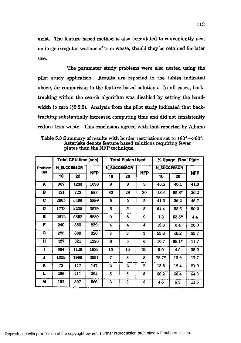
113

exist. The feature based method is also formulated to conveniently nest

on large irregular sections of trim waste, should they be retained for later

use.

The parameter study problems were also nested using the

pilot study application. Results are reported in the tables indicated

above, for comparison to the feature based solutions. In all cases, back

tracking within the search algorithm was disabled by setting the band

width to zero (§2.2.2). Analysis from the pilot study indicated tha t back

tracking substantially increased computing time and did not consistently

reduce trim waste. This conclusion agreed with that reported by Albano

Table 5.3 Summary of results with border restrictions set to 180“—>360°. Asterisks denote feature based solutions requiring fewer plates than the NFP technique.

ProblemSet

Total CPU time (sec) Total Plates Used % Usage Final Plate

N.SUCCESSORNFP

N.SUCCESSORNFP

N.SUCCESSORNFP

10 20 10 20 10 20

A 967 1283 1698 9 9 9 40.5 40.1 41.0

B 451 723 993 30 29 30 18.4 65.8* 26.2

C 2665 5406 5899 5 5 5 41.3 36.2 45.7

D 1773 2235 3579 5 5 5 54.4 53.6 50.2

E 2912 5852 8889 9 8 9 1.3 53.6* 4.4

F 240 380 239 4 4 4 13.3 6.4 20.0

G 285 388 320 3 3 3 53.8 46.2 55.7

H 407 821 1296 6 5 6 10.7 68.1* 11.7

1 664 1128 1629 10 10 10 9.0 4.0 38.0

J 1058 1999 3691 7 8 8 78.7* 12.9 17.7

K 73 117 147 2 2 2 13.5 12.4 21.0

L 266 411 394 5 5 5 60.2 60.4 64.9

M 192 397 586 3 3 3 4.6 5.9 11.6


114

and Sapuppo [ÂLBA80]. Elimination of the backtracking component also

permitted a more straightforward comparison of the two methods, based

on the merits of the NFP and shape based techniques.

Several observations can be made from Table 5.5, which

shows normalized CPU times for all cases of the study. Computation

times for the feature based solutions are lower than those of the NFP

technique. When using an NFP approach, a tentative placement for each

of the remaining available parts must be generated at every stage of the

solution. In theory, CPU time increases quadratically as a function of the

Table 5.4 Summary of results with border restrictions alternating between 90“-^ 180° and 180°-»270°. Asterisks denote feature based solutions requiring fewer plates than the NFP technique.

ProblemSet


N.SUCCESSORNFP

N.SUCCESSORNFP

N.SUCCESSORNFP

10 20 10 20 10 20

A 459 1000 1698 9 9 9 40.5 40.5 41.0

B 462 674 993 29 29 30 65.8* 65.8* 26.2

C 2062 3040 5899 5 5 5 31.2 34.1 45.7

D 977 1880 3579 5 5 5 54.6 37.1 50.2

E 1337 3339 8889 8 8 9 56.2* 45.8* 4.4

F 139 225 239 4 4 4 9.7 6.4 20.0

G 159 323 320 3 3 3 51.1 47.9 55.7

H 279 440 1296 6 5 6 2.7 61.9* 11.7

I 453 814 1629 10 9 10 10.7 62.3* 38.0

J 603 1999 3691 8 8 8 12.2 12.9 17.7

K 43 117 147 2 2 2 12.6 12.4 21.0

L 185 411 394 5 5 5 60.2 60.4 64.9

M 173 397 586 3 3 3 10.1 5.9 11.6


115

total number of profiles nested (§2.4). Over the course of a solution, a de

crease in CPU time firom plate to plate is evident, as a decreasing number

of parts are available. This trend is seen in Tables 5.6 and 5.7 where

CPU times per part are shown for each plate in the NFP solution for two

representative problems. The corresponding layouts are depicted in Fig

ures 5.5 and 5.6.

For the shape based heuristic an increase in parts corre

sponds to an increased number of matching indices. Calculating indices

accounts for a small percentage (5% to 10%) of total CPU time. For the

Table 5.5 Summary of CPU time per part reslut for the parameter study

ProblemSet

CPU Time Per Part (sec)

Numberof

Parts

N_SUCCESSOR = 10 N.SUCCESSOR = 20NFP180°

- »360°

90°-»180°<=>

180°-»270°

180°- »

360°

90°-*180°<=>

180°-+270°

A 13.81 6.56 18.33 14.29 24.26 70

B 4.14 4.24 6.63 6.18 9.11 109

C 12.94 10.01 26.24 14.76 28.64 206

D 17.21 9.49 21.70 18.25 34.77 103

E 9.87 4.53 19.84 11.32 30.13 295

F 4.62 2.67 7.31 4.33 4.60 52

G 3.39 1.90 4.62 3.85 3.81 84

H 7.27 4.98 14.66 7.86 23.14 56

1 6.21 4.23 10.54 7.61 15.22 107

J 9.53 5.43 18.01 18.01 33.25 111

K 1.97 1.16 3.16 3.16 3.97 37

L 5.12 3.56 7.90 7.90 7.58 52

M 2.82 2.54 5.84 5.84 8.62 68

TOTALS 8.85 5.43 15.66 10.86 21.75 1350


116

current application, evaluation of the successor waste functions represent

the largest portion of computation time (60%-80%). However, since at

each stage these calculations are capped by the total number of allowed

successors (NJSUCCESSOR), solution times are less adversely effected

by the number of parts. CPU times per part remain relatively equal over

the course of a solution, while total CPU time roughly doubles as the

number of successors varies from 10 to 20.

Table 5.6 Individual plate results for problem set C (Figure 5.5).N.SUCCESSOR equals 20.

PlateNumber

CPU Time Per Part Number of Parts % Trim Loss180“->

360”

90° 180“180®- 27(r NFP

180”

360”

90» 180"o

180''-»270° NFP180” —»

360”

90°-»180°CO

180*-»270 NFP

1 29.0 12.4 45.8 53 57 64 20.29 21.74 23.91

2 16.6 27.2 31.0 49 57 66 18.12 21.74 26.81

3 38.2 8.8 26.7 56 51 26 28.99 26.81 34.06

4 21.4 9.2 6.5 33 27 25 34.78 29.71 26.81

5 14.3 6.1 2.6 15 14 25 63.77 65.94 54.35

Table 5.7 Individual plate results for problem set H (Figure 5.6). N.SUCCESSOR equals 20.

P la teN um ber

CPU Time Per Part Number of Parts %Trim Loss180”->

360”

90°-»180*o

180'-»270” NFP180”-»

360”

g0'>-»i80»«»

180°-»270° NFP180”-»

3 6 0 ”

90°-+180”CO

180**-»270* NFP

1 18.1 8.0 30.9 10 15 12 40.1 31.37 28.98

2 16.0 6.0 33.0 13 10 14 38.3 35.73 37.47

3 12.3 10.8 24.5 11 12 11 30.8 26.36 37.15

4 15.9 6.0 10.7 10 10 11 23.1 32.68 35.62

5 11.6 7.8 12.6 12 9 6 31.9 38.13 36.71

6 N/A N/A 0.3 N/A N/A 2 N/A N/A 88.34


CD■DOQ.C

gQ.

■DCD

C/)

o'3O

8"O( O '3"i3CD

3.3"CD

CD■DOQ.CaO3

"Oo

CDQ.

(A) (B)

R

(C)

Q 0—0 O

Q—O__0__0

JX

"DCD

(/)(/)

Figure 5.5 Solutions for Problem C. Case (A): N_SUCCESSOR = 20, Border Restrictions 180“->360“. Case (B): N_SUCCESSOR = 20, Border Restrictions alternate between 90“—>180“ & 180“—>270“. Case (C); Pilot study results.

73CD■DOQ.C

gQ.

■DCD

C/)C/)

CD

8

3.3"CD

CD■DOQ.CaO3"OO

CDQ.

■DCD

C/)C/)

(B) (C)

0 ^ !

y

F\rC 'i ^ o _ o -)

% ;— ^

Figure 5.6 Solutions for Problem H. Case (A): N_SUCCESSOR = 20, Border Restrictions 180°-^360°. Case (B):N_SUCCESSOR = 20, Border Restrictions alternate between 90°—>180° & 180°—>270°. Case (C): Pilot {lî study results.

119

As seen in Tables 5.2 and 5,3, reducing the number of suc

cessors will sometimes adversely affect the solution. Placements are gen

erated in order from most to least favorable matching index. However,

since the indices are only an estimate of the quality of fit between the

part and void, there is no guarantee that the initial placements indicated

will be best. Consequently, an adequate pool of valid placements from

which to choose must be generated. Extra successors raise the probabil

ity of finding a better solution, however the additional benefit diminishes

with each new placement. In practice the value of N_SUCCESSOR is set

to produce a balance between the required quahty of nest and the desired

computation time.

Interestingly, the increased computation time associated

with more successors does not always produce improved layouts. An ex

ample is shown in Figure 5.7, where one less stock plate is needed by the

solution accessing ten fewer successors at each stage of the solution.

Such inconsistencies are related to the difficulty of predicting the future

effect of each successor. The waste function must forecast each place

ment’s influence on fiiture allocations, based solely upon the shape of the

current remaining resource. As a result, the generation of additional suc

cessors will occasionally allow the selection and expansion a less favor

able solution.

Another trend seen in the parameter study data were

smaller CPU times for cases where border shift restrictions alternated be

tween 90°to 180° and 180° to 270°. This result can be explained in part

by the effect of the restrictions on the formation of the remaining re

source. A single range of 180° to 360° forces parts to migrate toward the


120

ü

n n

CD

IIÏÏlrx-QJ

m

ün

T7û

o r-L

m

b-Tzrcrm

&Ha-crcrm

ôTo

0

oo

S

OQ 0

G

II

iCQ8

I

Iü01s if H CQ

i|OJ 04

|s'B g

| SCD

. OH? CQ

IIII,155

I m

II

d) enœ oc-U5

Ik


121

lower comers of the stock (Figure 5.5 case A). By contrast, the alternat

ing case causes parts to favor the left side of the plate (Figure 5.5 case B).

In the former situation, the leading edge of the solution tends to extend

along the length (longer side) of the plate, while for the later it spans the

height (shorter side). Remaining voids for the 180° to 360° case are gen

erally more complex and require larger CPU times for evaluation of their

waste functions.

5.5.2 Analysis o f All Cases

Based on the result of the parameter study a complete run of

the 42 industry problems was conducted with 20 successors and alternat

ing shift restrictions as above. Number of parts, computation time, total

resources required, and percent usage on the final plate are shown for

each problem in Table 5.8, along with values firom the pilot study applica

tion.

Total CPU time to place the 3,014 parts was 8.06 hours for

the feature based method, while the NFP technique required 11.46. For

35 of the problems, both methods required the same number of stock

plates. In six of the remaining seven problems, the feature based tech

nique required one less resource. The NFP technique used fewer stock

plates (1) in only one of the 42 problems. Representative examples of the

feature based solutions are plotted in Appendix A.3, with corresponding

examples of the NFP method found in A.4.

Material usage on final plates for both methods was also in

vestigated. Data firom both techniques was adjusted to produce a valid

comparison. When either method required one less resource, percent us

age on the final plate for that technique was considered zero. This is a


122

conservative measure as it ignores the available material remaining on

tha t solution’s true last plate. Solutions requiring one plate were ignored,

as material usage is identical for both methods and does not indicate the

quahty of packing achieved. Using these analysis criteria an average ma

terial savings of 4 percent was reahzed on the final plate of feature based

solutions.

Table 5.8 Results for all cases. N.SUCCESSOR equals 20. Border restrictions alternate between 90“ 180 '’ and 180°—>270°.

ProblemSet

Numberof

Parts


SHAPEBased

NFPBased

SHAPEBased

NFPBased

SHAPEBased

NFPBased

1-A 70 1300 992 9 9 40.5 41.0

2-B 109 694 993 29 30 65.8* 26.23 411 2355 751 56 55 26.9 26.9*

4 10 35 6 3 3 2.8 1.35 42 347 101 2 3 81.9* 9.4

6-C 206 3080 5899 5 5 34.1 45.7

7 6 50 1 1 1 8.0 8.0

8 15 65 8 2 2 42.8 39.1

9 156 1580 864 6 6 49.3 38.4

10 1 1 1 1 1 45.7 45.7

11 344 2602 4107 14 15 63.0* 11.412 4 7 1 4 4 44.0 44.0

13-D 103 1837 3577 5 5 37.1 50.214 34 376 269 3 3 8.7 8.815 3 14 1 1 1 9.5 9.516 76 887 778 2 2 60.8 63.6

17-E 295 4915 8889 8 9 45.8* 4.418 4 38 1 1 1 9.8 9.819 76 831 1226 5 5 61.2 55.0

* Required one less plate than other corresponding solution

(table con’d.)


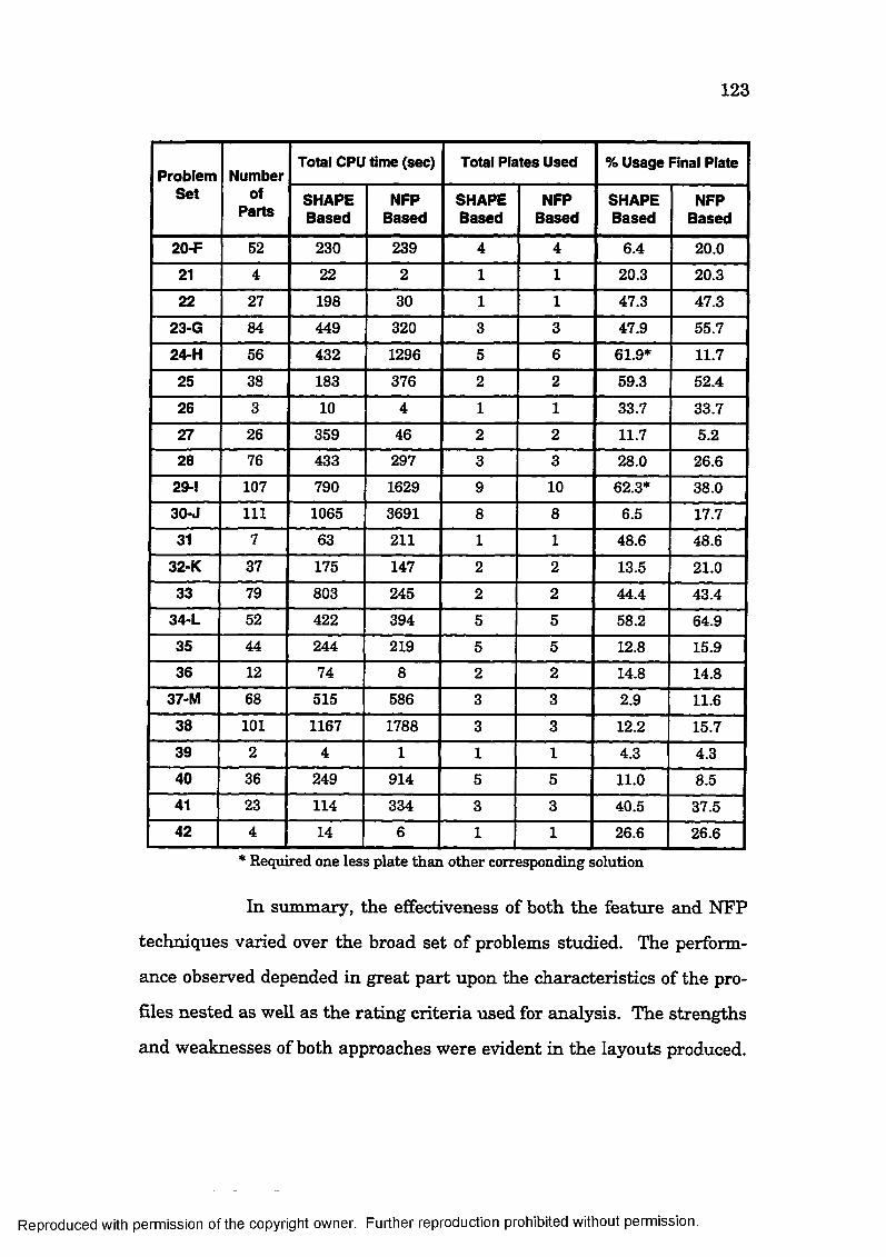
123

ProblemSet

Numberof

Parts


SHAPEBased

NFPBased

SHAPEBased

NFPBased

SHAPEBased

NFPBased

20-F 52 230 239 4 4 6.4 20.021 4 22 2 1 1 20.3 20.322 27 198 30 1 1 47.3 47.3

23-G 84 449 320 3 3 47.9 55.724-H 56 432 1296 5 6 61.9* 11.725 38 183 376 2 2 59.3 52.426 3 10 4 1 1 33.7 33.727 26 359 46 2 2 11.7 5.228 76 433 297 3 3 28.0 26.6

29-1 107 790 1629 9 10 62.3* 38.030-J 111 1065 3691 8 8 6.5 17.731 7 63 211 1 1 48.6 48.6

32-K 37 175 147 2 2 13.5 21.033 79 803 245 2 2 44.4 43.4

34-L 52 422 394 5 5 58.2 64.935 44 244 219 5 5 12.8 15.936 12 74 8 2 2 14.8 14.8

37-M 68 515 586 3 3 2.9 11.638 101 1167 1788 3 3 12.2 15.739 2 4 1 1 1 4.3 4.340 36 249 914 5 5 11.0 8.541 23 114 334 3 3 40.5 37.542 4 14 6 1 1 26.6 26.6

* Required one less plate than other corresponding solution

In summary, the effectiveness of both the feature and NFP

techniques varied over the broad set of problems studied. The perform

ance observed depended in great part upon the characteristics of the pro

files nested as well as the rating criteria used for analysis. The strengths

and weaknesses of both approaches were evident in the layouts produced.


124

However, results generally indicate shorter computation times and better

packing from the proposed shape reasoning approach. Additional com

mentary is deferred to the next chapter where concluding remarks and

suggestions for further investigation are discussed.


C hapter 6 C onclusions and F uture Work6.1 Summary

The research presented in this manuscript confirms the fun

damental premise that an effective solution to the irregular profile bin

packing problem can be formulated using information about the configu

ration and shape of a layout’s parts. This shape information is stored in

the form of features, geometric constructs of two and three sides, which

are extracted firom both the unallocated part profiles and the region of the

stock resource remaining available for use. A series of simplification

techniques are applied to these entities, permitting the characterization

of shape at the various scales of detail required for solution reasoning.

Layouts are generated in an iterative fashion. At each stage

of nesting, all possible matches between the part and resource features

are examined for the possible existence of complementary forms. Using

the extracted shape information, a matching index is calculated to quan

tify the quality of fit achieved by each pair. Based on this measure, a set

of intermediate allocations is generated using those parts most likely to

produce efficient placements. The orientation and initial position of each

of the chosen parts is provided by the designated align type, a description

of the way in which two features mesh. A single layout for expansion in

the next stage of the solution is then selected using a waste function

which predicts the current and future trim loss associated with each ar

rangement.

125


126

The utility of the technique described has been demon

strated through testing on a diverse set of industry supplied problems. A

comprehensive inspection of the feature based layouts generated indi

cates nests of comparable waste which are commonly superior to those of

the NFP method. Individual nests within the feature base results will

often exhibit exceptionally low wastes previously un-achieved using the

NFP approach. However, the comparison of two techniques through the

examination of individual plates is often misleading, as the parts found

on each plate differ from solution to solution. Overall results from the

complete set of resources used must also be considered.

Furthermore, no standard data sets exist on which to per

form benchmark runs. Such issues complicate the appraisal of any nest

ing technique’s merits. However, based on results from the total run of

42 problems, the relative merits of this technique are evident. On aver

age, solutions requiring less stock material were produced at less compu

tational expense.

6.2 Shape R easoning Advantages and L im itations

An integral part of all packing problem solution algorithms

is an ability to deal with the infinite number of placement possibilities oc

curring throughout the generation of a layout. Many researchers have

coped with this task by limiting the available options at the outset. Al

though effective, this approach automatically restricts the number and

type of solutions capable of being produced. The current method provides

additional flexibility by avoiding the restrictions commonly used to yield

computationally tractable solutions.


127

The most striking difference between the proposed method

and previous reported techniques, is the abihty to dynamically select opti

mal part orientations. This differs from the majority of techniques, such

as the NFP, which restrict profiles to a distinct set of normally orthogo

nal rotations. Furthermore, a t each stage of the solution the current for

mulation permits the selection and placement of any available part. This

contrasts with other approaches which either allocate in a specific prede

termined order or break the complete profile set into smaller more work

able problems.

As is common with many heuristic methods, the documented

shape reasoning approach mimics tha t of a human nester. The skilled

eye of a technician can quickly scan a large set of profiles and easily de

tect the complementary shapes which exist between the parts and re

maining resource. The success of the proposed algorithm stems from its

ability to imitate this manual technique. Detection of the underlying pro

file shapes is made possible through elimination of unnecessary and con

fusing detail. With this accompUshed all information can easily be stored

in a basic feature format. Determination of the plausible part orienta

tions and locations are then made quickly using matching indexes and

align types. This avoids the brute force approach of the NFP technique,

whereby a series of placements must be generated for all parts regardless

of their merit. The finer details of parts are also retained however, and

exploited during final placement. Here, the removal of any unnecessary

space is made possible through the shifting and abutting of the complex

original profiles.


128

One trend observed in both the NFP and feature based re

sults was a noticeable increase in trim waste as solutions progressed from

one plate to the next for a selected set of profiles. This can be attributed

to the early depletion of smaller more easily placed parts which can fill

gaps or recesses. For later plates what remains are usually large and

highly irregular profiles. As parts become larger relative to the resource,

much of the flexibility associated with feature based placement cannot be

exploited, as the restrictions imposed by the boundary of the stock become

more pronounced. As a concequence, a substantial improvement over pre

vious methods for these later plates is sometimes not observed.

The efficient nesting of larger profiles often requires infor

mation about the future interaction of the parts to be allocated. Consid

erations must be made to combine multiple parts such that they conform

to or exploit the dimension of the resourse involved. The iterative place

ment of individual parts does not permit this. At each stage of the cur

rent method, the next placement is resolved based upon interactions be

tween single parts and the current configuration. Consequently predict

ing future effects is difficult. This limitation, however, is inherent in

most iterative placment techniques. Possible avenues of improvement are

suggested in the next section.

6.3 Future Work

In many cases the nests produced by the automated applica

tion can be improved through slight manual alteration, however the

waste recovered by such operations is often minimal. Any gains made

through manual interaction must be weighed against the increased costs

in man hours. In industry, nesting involves the optimization of both


129

material and labor used, as well as other issues including states of cutting

equipment, stock availability and scheduling. If the advantages of man

ual layout were merited, productivity could be gained by incorporating

the proposed techniques into a hybrid manual-automatic system. In such

an application, feature matching heuristics would be employed to quickly

provide a palate of suggested placements. Rather than depend upon a

calculated waste function, the full experience and intuition of the techni

cian could be exploited to select, and if necessary adjust the most promis

ing layout for expansion. The capability to manually generate placements

could also be integating into the application. Albano provides a detailed

outline of such a pseudo automatic system [ALBA77].

Throughout the evolution of this research, a constant objec

tive has been the development of a robust system capable of solving a di

verse set of "real world" problems. Experiments have verified the stabil

ity of the algorithms implemented for a broad set of complex inputs. As

with all system of this nature, tradeoffs must be made to accommodate

the broad range of cases which can occur. Specializing for a specific set of

characteristics is usually unwise, as such procedures invariably degrade

algorithm performance on other sets. As a consequence, the resulting ap

plication is optimal for fewer problems although competent for all. From

a practical viewpoint a dependable method is ofiæn preferable to a supe

rior one which sometimes fails.

Beyond the need to solve a spectrum of problems, other fac

tors prohibit the development of specialized optimum values for the toler

ances and parameters controlling algorithm performance. As the sim

plest of industry problems often contain non-uniform distributions of


130

profile characteristics, catering to the needs of even a single problem can

be difficult. Opportunities for such improvements might exist however, if

diverse and hard to manage problems could be transformed into sets with

a narrower assortment of properties. This task might be accomplished

through the clustering of complementary parts prior to nesting, assuming

such matching profiles exist. With problems converted to a simpler form,

investigation of optimal tolerance settings might be justified. Values for

those parameters controlling part feature generation, rem ain ing resource

simplification and matching index calculations could be determ in ed

through comparative runs of the application.

Another issue deserving additional study is determination of

the best successor for expansion. Although information firom the set of re

maining parts is used to dynamically control the waste fimction, it is still

inherently limited to examining only the current solution. Unfortunately,

the detrimental effect of certain placements can only be seen in successive

steps. One solution to such problems is to adopt a less deterministic

search algorithm which explores several potential paths at each stage of

the solution process. Unfortunately, results firom the backtracking tech

nique implemented in the pilot study indicated a substantial increase in

solution time without a consistent reduction in waste.

The potential benefits firom a new search method must be

weighed against the extra computational expense of evaluating any addi

tional part placements required. If the present formulation of the waste

function is to be used for such calculations, algorithms for determ in ing

the useful and un-usable areas of a layout must be optimized, as these

currently account for 60 to 80 percent of run times. An alternative would


131

be the use of a less rigorous waste function coupled with more exacting

m atching indexes. The additional information needed for new index for

mulations might be provided by further exploiting the geometry associ

ated with each aHgn type. Such an approach could be effective at elimi

nating less favorable placements.

The allocation of irregular shapes is a strongly domain de

pendent problem. As such, it is difficult if not impossible to develop ge

neric solution strategies which are optimal when applied to all cases. To

varying degrees, expert systems overcome this issue by addressing only

specific problem types. These solutions are effective but limited in appli

cation. Unfortunately in many industry no single approach is appropriate

for the full range of problems encountered. For this reason, the methods

presented throughout this document have attempted to deal with profile

allocation a t the most fundamental of levels, using the individual shape of

parts. However, by ignoring the overall character of the problem studied,

potential clues to the best method may be lost. In the future, intelligent

systems will qualify the nature of a problem during processing, permit

ting apphcation of the most appropriate method available. The shape

reasoning heuristics developed will provide usefiil tools for accomplishing

this task, adding to the arsenal of methods available for solving this com

plex problem.


B ibliography[ADAM76] Âdamowicz, M., Albano, A. "A Solution to the Rectangular

Cutting-Stock Problem", IEEE Transactions on Systems, Man & Cybernetics, April 1976, pp. 302-310.

[ADAM791 Adamowicz, M., Albano, A. "Nesting Two-dimensional Shapes in Rectangular Modules", Computer Aided Design, No. 2, Vol. 8, April 1979, pp. 27-33.

[ALBA77] Albano, A., "A Method to Improve Two-dimensional Layout", Computer Aided Design, Vol. 9, No. 1, January 1977, pp. 48-52.

[ALBA80] Albano, A., Sapuppo, Giuseppe, "Optimal Allocation of Two-Dimensinal Inregiilar Shapes Using Heuristic Search Methods", IEEE Transactions on Systems, Man & Cybernetics, May 1980, pp. 242-248.

[ARBE93] Arbel, Ami, "Large -Scale Optimization Methods Applied to the Cutting Stock Problem of Irregular Shapes", International Journal o f Production Research, Vol. 31, No. 2, 1993, pp. 483-500.

[BENG82] Bengtsson, Bengt-Erik, "Packing Rectangular Pieces - A Heuristic Approach", The Computer Journal, Vol. 25, No. 3, 1982, pp. 353-357.

[BOWY93] Bowyer, Adrian, & Woodwork, John, Introduction to Computing with Geometry, Information Geometers Ltd., Winchester UK, 1993.

[BRON83] Bronsoiler, A., Sanders, J.L., "Performance Testing ofIrregular Parts Nesting Systems for Flame Cutting and Other Industrial Applications", 1983~SME ManufacturingEngineering Transactions 11th NAMRC North AmericanManufacturing Research Conference Proceedings, pp. 434-440.

[CAME86] Cameron, S.A., CuUey, R. K., "Determining the Minimum Translational Distance Between Two Convex Polyhedra", CH2282-2/86/0000/05911986 IEEE, pp. 591-596.

[CAVI89] Caviglia, Daniele D., Bisio, Giacomo M., Curatelli,Francesco, Giovannacci, Luca, & Raffo, Luigi, "NeuralAlgorithms for Cell Placement in VLSI Design", Proceedingso f International Joint Conference on Neural Networks, 1989,IEEE Catalog Number 89CH2765-6, pp. 1573 - 1580.

132


133

[CHE091] Cheok, B.T., and Nee, Y.C., "Algorithms for Nesting of Ship/Ofifehore Structural Plates", Advances in Design Automation -1991-, DE-Vol. 32.-2, ASME, pp. 221-226.

[CHEI77] Christofides, Nicos, & Whitlock, Charles, "An Algorithm for Two-Dimensional Cutting Problems", Operations Research, Vol. 25, No. 1, Januaiy-February 1977, pp. 30-44.

[CHUN89] Chung, Jason, & Hillman, Danald J., "Object Oriented Nesting System on Two-dimentional Highly Irregular Resoruces", Intelligent Robots and Computer Vision VIII: Systems and Applications, SPEE Vol. 1193, 1989, pp. 54-63.

[COFF90] CoiB&nan, E.G., & Shor, P. W., "Average-case Analysis of Cutting and Packing in Two Dimensions", European Journal of Operational Research, Vol. 44, No. 2, January 25, 1990, pp. 134-144.

[DAGL83] Dagli, Cihan H., & Totoglu, M. Yalcin, "A Computer Package for Solving Cutting Stock Problems", 7th International Conference on Production Research, Windsor, Ontario, Canada, Vol. 1,1983, pp. 480-486.

[DAGL87] Dagli, Cihan, & Tatoglu, M. Yalcin, "An approach to Two-Dimensional Cutting Stock Problems", International Journal o f Production Research, Vol. 25, No. 2, 1987, pp. 175-190.

[DAGL88] Dagh, Cihan, "Cutting Stock Problem: Combined Use ofHeuristics and Optimization Methods", Recent Developments in Production Research, A. Mital editor, Elsevier Science Publishers B.V., Amsterdam, 1988, pp. 500-506.

[DAGL90a] Dagli, Cihan, Hajakbari, Alireza, "Parallel Architecture for Stock Cutting Problem", PARABASE 90 Int Conf Databases Parallel Archit Appl PARABASE 90: InternationalConference on Databases, Parallel Architectures, and Their Applications, Miami Beach, FL, USA, Mar 7-9 1990 (IEEE cat n 90CH2728-4) CH2728-4/90/0000/0534 1990 IEEE, p. 534.

[DAGL90b] Dagli, Cihan H., & Hajakbari, Alireza, "Simulated Annealing Approach for Solving Stock Cutting Problems", Proceedings of IEEE International Conference on Systems, Man, and Cybernetics, 1990, IEEE Catalog Number 90CH2930-6, pp. 221-223;


134

[DAVI77] Davis, Larry S., "Understanding Shape: Angles and Sides", IEEE Transactions on Computers, Vol. c-26. No. 3, March 1977, pp. 236-242.

[DECA78] DeCani, Phillip, "A Note on the Two-dimensional R e c ta n ^ a r Cutting-stock Problem", Journal o f the Operational Research Society, Vol. 29, No. 7, 1978, pp. 703-706.

[DDET91] Dietrich, Robert D., & Yakowitz, Sidney J., "A Rule-Based Approach to the Trim-Loss Problem", International Journal of Production Research, Vol. 29, No. 2,1991, pp. 401-415.

[DYCK90] Dyckhoff, Harald, "A Typology of Cutting and Packing Problems", European Journal o f Operational Research, Vol. 44, No. 2, January 25,1990, pp. 145-159.

[DYCK92] Dyckhoff, Harald, & Finke, Ute, Cutting and Packing in Production and Distribution A Typology and Bibliography, Physica-Verlag, A Springer-Verlag Company, Heidelberg, 1992.

[FARL90] Farley, Alan A., "The Cutting Stock Problem in the Canvas Industry", European Journal o f Operational Research, Vol. 44, No. 2, January 25,1990, pp. 247-255.

[FOLE84] Foley, James D., & Van Dam, Andries, Fundmentals o f Interactive Compter Graphics, Addison Wesley Publishing Company, Reading, Massachusetts, 1984.

[FREE64] Freeman, H., & Carder, L., "Apictorial Jigsaw Puzzles: The Computer Solution of a Problem in Pattern Recognition", IEEE Transactions on Electronic Computers, Vol. 13, 1964, pp. 118-127.

[FREE74] Freeman, Herbert, "Computer Processing of Line-Drawing Images", Computing Surveys, Vol. 6, No. 1, March 1974, pp. 57-97.

[FREE75a] Freeman, H., & Shapira, R., "Determining theMinimum-Area Encasing Rectangle for an Arbitrary Closed Curve", Communications o f the ACM, Vol. 18, No. 7, July 1975, pp. 409-413.

[FREE75b] Freeman, Herbert, "On the packing of Arbitrary-Shaped Templates", Second USA-JAPAN Computer Conference, 1975, pp. 102-107.


135

[FREE78] Freeman, Herbert, "Shape Description Via the Use of Critical Points", Patem Recognition, Vol. 10, 1978, pp.159-166.

[FUJI93] Fujita, Kikuo, Akagi, Shinsuke, & Hirokawa, Noriyasu,"Hybrid Approach for Optimal Nesting Using a Genetic Algorithm and a Local Minimization Algorithm", Advances in Design Automation, Vol. 1, ASMS 1993, pp. 477-484.

[GANT93] Ganter, MA., & Skoglund, P A , "Feature Extraction forCasting Core Development", ASME Journal o f Mechanical Design, Vol. 115, December 1993, pp. 744-750.

[GARE79] Garey, Michael R., & Johnson, David S., Computers and Intractability, W.H. Freeman and Company, San Francisco, 1979.

[GEMM92] Gemmill, Douglas D., "Solution to the Assortment Problem Via the Genetic Algorithm", Mathematical and Computer Modeling, Vol. 16, No. 1,1992, pp. 89-94.

[GnJL65] Gilmore, P.C., & Gomory, R.E., "Multi-Stage Cutting StockProblems of Two and More Dimensions", Operations Research, Vol. 13,1965, pp. 94-120.

[GONZ78] Gonzalez, Rafael C., & Thomason, Michael G., SyntacticPattern Recognition an Introduction, Addison-Wesley, London, 1978. Chapter 6, Pavlidis, T., & Feng, H.Y.F., "Shape Discrimination", pp 125-144.

[HAES91] Haessler, Robert W., & Sweeney, Paul E., "Cutting StockProblems and Solution Procedures", European Journal o f Operational Research, Vol. 54,1991, pp. 141-150.

[HAHN68] Hahn, Susan G., "On the Optimal Cutting of DefectiveSheets", Operations Research, Vol. 16, No. 8, 1968, pp. 1100-1114.

[HAIM70] Haims, Murray J., Freeman, Herbert, "A Multistage Solutionto the Template-Layout Problem", IEEE Transactions on Systems Science & Cybernetics, April 1970, pp. 145-151.

[HART85] Hartigan, P.M., "Computation of the Dip Statistict Test forUnimodality", Applied Statistics, Vol. 34,1985, pp. 320-325.

[HXLL90] Hill, Fransis S., Computer Graphics, Macm illan PublishingCompany, New York, 1990.


136

[BŒNX80] Hinxman, A.I., "The Trim-loss and Assorment Problems: A Survey", European Journal o f Operational Research, 5 (1980), pp. 8-18.

[H0R075] Horowitz, Steven L., "A Syntactic Algorithm for PeakDetection in Waveforms with Applications to Cardiography", Communications o f the ACM, Vol. 18, No. 5, May 1975, pp. 281-285.

[ILLI89] niiev, V.I., Popov, G.S., Ivanov, M., "A System forComputer-aided Technical Preparation in the Production of Plane Parts by Stamping", Journal o f Mechanical Working Technology, 18 (1989), pp. 283-292.

[ISRA82] Israni, Sharat, Sanders, Jerry, "Two-dimensional CuttingStock Problem Research: a Review and a New Rectangular Layout Algorithm", Journal o f Manufacturing Systems, Vol. 1, No. 2, pp. 169-182.

[ISRA85] Israni, Sharat S., Sanders, Jerry L . , "Performance Testing ofRectangular Parts-nesting Heuristics", International Journal o f Production Research, 1985, Vol. 23, No. 3, pp. 437-456.

[JAIN92] Jain, P., Fenyes, P., Richter R., "Optimal Blank NestingUsing Simulated Annealing", Journal o f Mechanical Design (Transactions of the ASlVffi ), March 1992, Vol. 114, pp.160-165.

[KAMP88] Kampke, Thomas, "Simulated Annealing: Use of a New Toolin Bin Packing", Annals o f Operations Research, Vol 16., 1988, pp. 327-332.

[KERK83] Kirkpatrick, S., Gelatt, C D., & Vecchi, M.P., "Optimizationby Simulated Annealing", Science, Vol. 220, No. 4598, May 13, 1983, pp. 671-680.

[LAM086] Lamousin, H.J., Waggenspack, W.N., & Dobson, G.T."Nesting of (Complex 2-D Parts Within Irregular Boundaries", Journal o f Manufacturing Science and Engineering, August 6,1986

[LOZA83] Lozano-Perez, Tomas, "Spatial P lanning: A ConfigurationSpace Approach", IEEE Transactions on Computers, Vol. C-32, No. 2, February 1983, pp. 108-120.


137

[LUTF92] Lutfîyya, Hanan, McMillin, Bruce, Poshyananda, Pipatpong, & Dagli, Cihan, "Composite Stock Cutting Through Simulated Annealing", Mathematical and Computer Modeling, Vol. 16, No. 1,1992, pp. 57-74.

[NEE86] Nee, A.Y.C., Seow, K.W., Long, S.L. "Designmg Algorithm for Nesting Irregular Shapes With and Without Boundary Constraints", Annals o f the CIRP, Vol. 35/1/1986, pp. 107-110.

[NEE88] Nee, A.Y.C., Long, S.L., "Microcomputer-aided MaterialManagement in a Furniture Factory", Computers in Industry, 10 (1988), pp. 221-229.

[NIEV82] Nievergelt, J, Preparata, F.P., "Plane-Sweep Algorithms forIntersectin Geometric Figures", Communications o f the ACM, October 1982, Vol. 25, Number 10, pp. 739-747.

[N0AK91] Noaker, Paula, "Software tha t Packs a Punch. CAD/CAM tools allow fabrication parts ju st in time". Manufacturing Engineering, Vol. 107, No. 5, November 1991, pp. 93-96.

[OLIV90I Oliveira, Jose Fernando, Ferreira, Jose Soeiro, "AnImproved Version of Wan^s Algorithm for Two-Dimensional Cutting Problems", European Journal o f Operational Research, Vol. 44, No. 2, January 25,1990, pp. 256-266.

[PAVL73] Pavlidis, Theodosios, 'Waveform Segmentation ThroughFunctional Approximation", IEEE Transactions on Computers, Vol. c-22. No. 7, July 1973, pp. 689-697.

[PAVL74] Pavlidis, Theodosios, & Horowitz, Steven L., "Segmentationof Plane Curves", IEEE Transactions on Computers, Vol. c-23. No. 8, August 1974, pp. 860-870.

[PAVL78] Pavlidis, Theodosios, "Survey A Review of Algorithms forShape Analysis", Computer Graphics and Image Processing, Vol. 7,1978, pp. 243-258.

[PAVL80] Pavlidis, T., Structural Pattern Recognition, Springer VerlagSeries in Electrophysics, Springer Verlag, Berlin, Heidleberg, New York, 1980.

[POSH90] Poshyanonda, Pipatpong, Bahrami, Ali, & Dagli, Cihan H.,"Two Dimensional Nesting Problem: Artificial NeuralNetwork and Optimization Approach", Proceedings o f 1990 IEEE International Confemce on Systems, Man, and Cybernetics, November 4-7, 1990, IEEE Catalog Number 90CH2930-6, ISBN 0-87942-597-0, pp. IV 572 - IV 577.


138

[PRAS91] Prasad, Y.K.D.V., Somasundaram, S. "CASNS - A Heuistic Algorithm for the Nesting of Irregular-Shaped Sheet Metal Blanks", Computer Aided Engineering Journal, Vol. 8, No. 2, April 1991, pp. 69-73.

[PRAS94] Prasad, Y.K.D.V., "A Set of Heuristic Algorithms for Optimal Nesting of Two-Dimensional Irregularly Shaped Sheet-Metal Blanks", Computers in Industry, 24 (1994), pp. 55-70.

[PREP85] Preparata, Franco P., & Shamos, Michael Ian,Computational Geometry an Introduction, Springer-Verlag, New York, Berlin, 1985.

[QU87] Qu, Weishuang, Sanders, Jerry, "A Nesting Algorithm forIrregular Parts and Factors Affecting Trim Losses", Interanational Journal o f Production Research, 1987, Vol. 25, No. 3, pp. 381-397.

[QU89] Qu, Weishuang, Sanders, Jerry L., "Sequence Selection ofStock in Two-Dimensional Layout Problems", International Journal o f Production Research, 1989, Vol. 27, No. 9, pp. 1553-1571.

[RADA82] Radack, Gerald M. & Badler, Norman I., "Jigsaw PuzzleMatching Using A Boundary-Centered Polar Encoding", Computer Graphics and Image Processing, Vol. 19, 1982, pp. 1-17.

[RINN87] Rinnooy Kan, A.H.G., DeWit, J.R., and Wijmenga, R.Th.,"Nonorthogonal Two-Dimensional Cutting Patterns", Management Science, Vol. 33, No. 5, May 1987, pp. 670-684.

[ROSE73] Rosenfeld, Azriel, & Johnston, Emily, "Angle Detection onDigital Curves", IEEE Transactions on Computers, September 1973, pp. 875-878.

[ROSE75] Rosenfeld, Azriel, & Weszka, Joan, "An Improved Method ofAngle Detection on Digital Curves", IEEE Transactions on Computers, September 1975, pp 940-941.

[SAND88] Sandgren, E., Dworak, T., "Part Layout Optimization using aQuadtree Representation", Proceedings o f the 1988 Design Automation Conference, Kissimmee, Florida, pp. 211-219.

[SARI83] Sarin, S.C., "Two-Dimensional Stock Cutting Problems andSolutions Methodologies", Journal o f Engineering for Industry (Trans, of the ASME), August 1983, Vol. 105, pp. 155-160.


139

[SCHA78] Schachter, Bruce, "Decomposition of Polygons into Convex Sets", ŒEE Transactions on Computers, Vol. C-27, No. 11, November 1978, pp. 1078-1082.

[SERR82] Serra, J.Q. Image Analysis and Mathematic Morphology, Adison Wesley, New York, 1982.

[SHAH95] Shah, Jami, & Mantyla, Martti, Parametric and Feature Based CAD/CAM Concepts, Techniques, and Application, John Wiley & Sons Inc., New York, 1995.

[SHAM76] Shamos, Michael I., & Hoey, Dan, "Geometric IntersectionProblems", 17th Annual Symposium on Foundations o f Computer Science, Houston, 1976, pp. 208-215.

[SPER79] Sperling, B. "Nesting Is More Than a Layout Problem",Computer Applications in the Automation o f Shipyard Operation and Ship Design III, 1979, pp. 287-294.

[STAL83] Staley, S. M., Henderson, M.R., & Anderson, D. C., "UsingSyntactic Pattern Recognition to Extract Feature Information From a Solid Geometric Data Base", Computers in Mechanical Engineering, September 1983, pp. 61-66.

[SUMM87] Summer, Charles J., & McNamara, James N., "PowerConsiderations for the Dip Test of Unimodality Using Mixtures of Normal and Uniform Distributions", American Statistical Association 1987 Proceedings o f the Statistical Computing Section, 1987, pp. 186-191.

[SZYK95] Szykman, S. & Cagan, J., "A Simulated Annealing-BasedApproach to Three-Dimensional Component Packing", Journal o f Mechanical Design, June 1995, Vol. 117, pp. 308-314.

[YUZU87] Yuzu, Cai, Lujim, Liu, Wangwei, "An Expert System forAutomatic Allocation of 2D Iiregiilar Shapes", Proceedings o f Expert Systems in Computer Aided Design Conference, International Federation for Information Processing 1987, pp. 407-423.


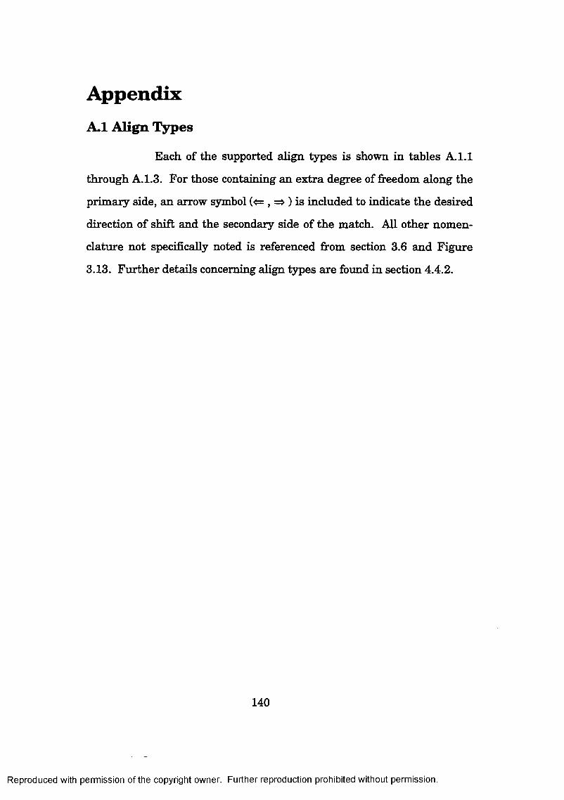
A ppendixA.1 A lign Types

Each of the supported align types is shown in tables A. 1.1

through A.1.3. For those containing an extra degree of freedom along the

primary side, an arrow symbol (<= , => ) is included to indicate the desired

direction of shift and the secondary side of the match. All other nomen

clature not specifically noted is referenced from section 3.6 and Figure

3.13. Further details concerning align types are found in section 4.4.2.

140


141

Table A.1.1 Align l^p es for Side One Alignment

AlignType

{ Q^p < Q^y) Class ReferenceVertex

ReferenceEdge

OtherConditions

lA '2P E IV <^BV

IB '2P 'IV ^B P ^ ®BV

1C NT 2P 'IV

fi m

ID NT '2P E IV

IE NT '2P E IV 0Bv> 0

IF '2P E IV 1 3 V - 0

"T" = Touching "NT" = Non T ou ch in g

(table con’d.)


142

ReferenceEdge

OtherConditions

ReferenceVertex

AlignType

Class

IG 2P 'BVIV

IH 'EY2P IV

NT 2P IV

NT 2P IV

IK NT 2P IV

IL 2P IV

"T" = Touching "NT" = Non Touching


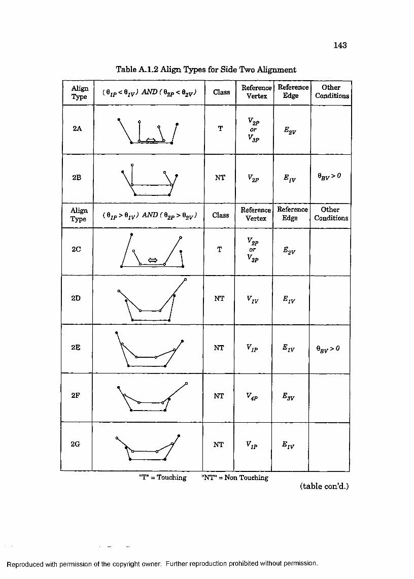
143

Table A. 1.2 Align Types for Side Two Alignment

AlignType ( ^ AND ( 2p ^ Class Reference

VertexReference

EdgeOther

Conditions

2A*'2Por3P

E.2V

2B NT 2P EIVQ g v > 0

AlignType Class

ReferenceVertex

Reference Edge

OtherConditions

2C*2Por E.

V.2V

3P

2D NT VIV EIV

2E NT 'IP nv 0gV-> 0

2F NT '4P E.3V

20 NT IP EIV

"T" = Touching "NT" = Non Touching(table con’d.)


144

AlignType ( ^ GjyJ AND ( 2P ^ ®2V- Class Reference

VertexReference

EdgeOther

Conditions

2H IP E.2V

21 NT '3P E3V

2J NT IP 'IV

AlignType Class

ReferenceVertex

ReferenceEdge

OtherConditions

2K '3P E.'2V

2L NT '2P EIV

2M NT '2P EIV 8^y > 0

"T" = Touching "NT" = Non Touching(table con’d.)


145

ReferenceEdge

OtherConditions

ReferenceVertex

AlignType

( Qjp < e^y) Class

2N 2P '2V

20 '2V2P

2P '2V3P

3P '2V



146

Table A.1.3 Align Types for Side Three Alignment

AlignType ( 8gp < Class Reference

VertexReference

EdgeOther

Conditions

3A '3P E3V

3B V,3P E.3V

3C

3----- »NT '3P E.3V

3D NT '3P E.3V

3E NT '3P 8jgy.>0

3F=5-*

'3P ■‘3V h v ~ 0


(table con’d.)


147

ReferenceEdge

OtherConditions

ReferenceVertex

AlignType

3G 3P 'BV'3V

3H 'BV'3V3P

NT 3P '3V

NT 3P '3V

NT3K 3P '3V

3L 3P '3V



148

A.2 A Sam ple Problem D escription

Figures A.2.1 through A.2.4 show a sample of the detailed

problem description output by the feature based application. The exam

ple depicted is for Problem I. Individual values within the distribution

are indicated by the black dots contained in each histogram bar. Futher

information concerning the subjects for each figure may be found in sec

tion 5.5.


149

Normalized Area Distribution

■2 5£

_a_5 10 15

Martnallzed P a rt Area x 100 56 Total P arts Average Normalize Area = 6.4

N orm alized Area Sum D istribution

20

£

£

£

10 15Normalized P art Area x 100

357 Total Normalized P art Area x 100

20

Figure A.2.1 The Normalized Area and Normalized Area Sum histograms.The height of each bar in the lower graph represents the sum of area values from corresponding range in the distribution above.


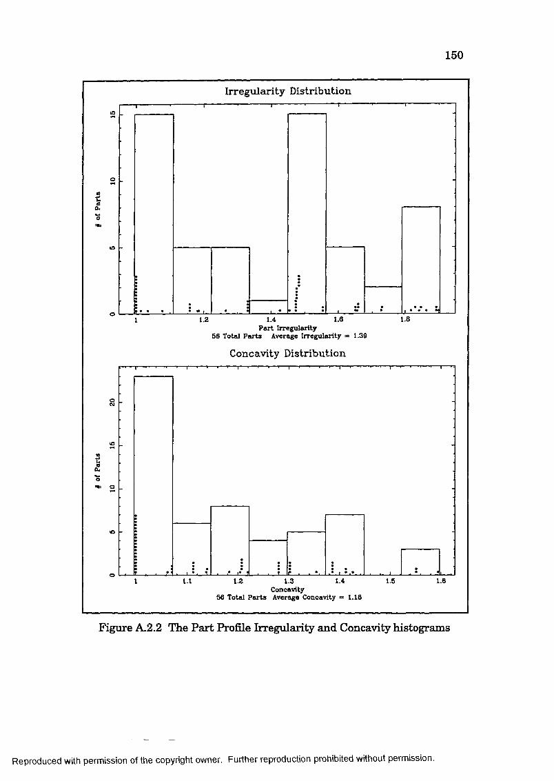
•o .

ao.

Irregu larity D istribution

1.2 1.4 1.6P a rt Irregularity

56 Total P arts Average Irregularity = 1.39

Concavity Distribution

t*. I

150

1.8

1.1 1.2 1.41.3 Concavity

56 Total P arts Average Concavity = 1.18

1.5 1.6

Figure A.2.2 The Part Profile Irregularity and Concavity histograms


<£

£ o

Aspect Ratio D istribution

_ u _1.5 2.5

Aspect Ratio 56 Total Parts

Part Complexity D istribution

? ? T10 15 20Number of Profile Vertices

56 Total Parts Average Complexity = 12.1

151

3.5

25

Figure A.2.3 The Aspect Ratio and Part Complexity histograms


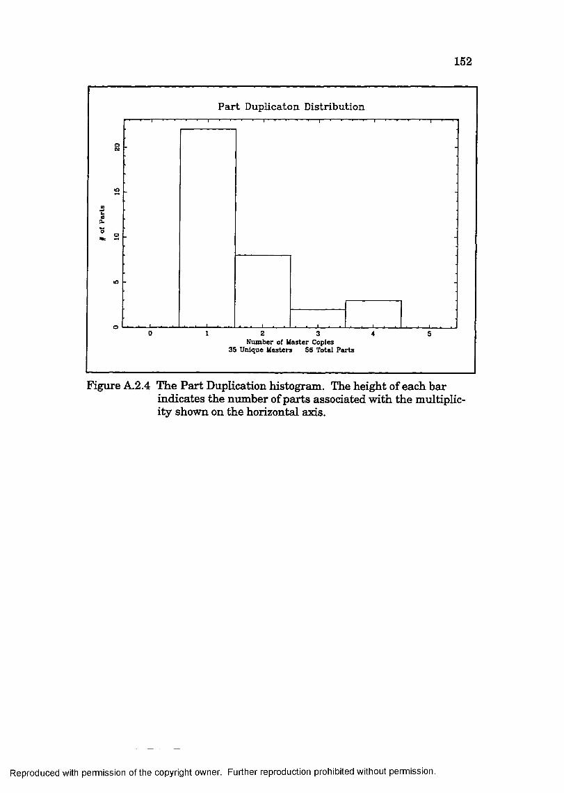
152

P art D uplicaton D istribution

OCV}

j2£

o

0 1 2 3 4 5Number of Waster Copies

35 Unique Wasters 56 Total Parts

Figure A.2.4 The Part Duplication histogram. The height of each barindicates the number of parts associated with the multiplicity shown on the horizontal axis.


153

A.3 F eature Based Solution Layouts

Figures A.3.1 through A.3.13 show feature based solutions

for the problems of the parameter study. Layouts are plotted in the order

of their creation from left to right across each row. N_SUCCESSOR is 20

with border restrictions alternating between 90“->180° and 180°-»270°.

Additional information for each problem concerning the profile character

istics, CPU times, and trim waste can be found in Tables 5.2, 5.4, and 5.5.


154

r i

<

iCO<

I


J L J L

O

155

?8to

pqÎ

IIMCO

<(1)

0


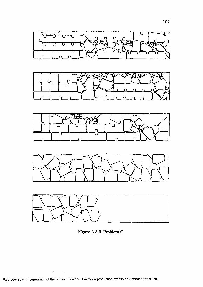
157

Figure A.3.3 Problem C


158

Figure A.3.4 Problem D


159

0

0

e

0

□

u-Hoo

o OOO

©__

o t Oo o

1 oo o(D o

) cDoeo Oo 0o

o

0

o o oo o o

C o oo o o

o o o

o0 0

oo

ooo

ooooo

oooooo

o

0 0

0o0

MI1£l£)co<

Is


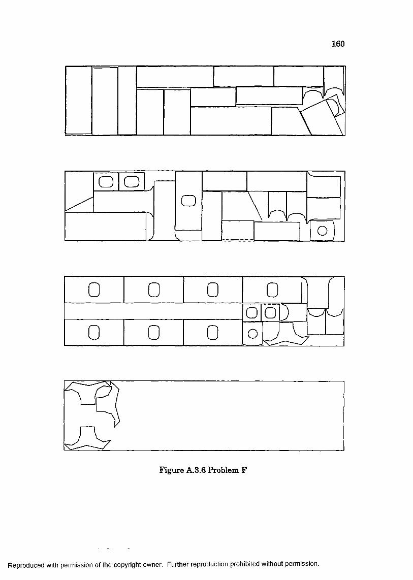
160

o o

Figure A.3.6 Problem F


161

^ 10 (o

o

0 0G

O

O

0 1 0o o

Figure A.3.7 Problem G


162

Figure A.3.8 Problem H


163

G

J

e

105CO

I


164

c r - C T T

O

kL—

Jd_CL

J Z lJZL 3

crcr-D

\

B L .

"-5i

ICO<

I


165

i " — —Y0 n.o 1 " 1 o

o—------ o : — — 1

Figure A.3.11 Problem K


166

r:o o

)

o o

Figure A.3.12 Problem L


167

O

1 .C1C10 0 _G[fn

-(OMO Gu ou c) Q O O O U"o o o U

Figure A.3.13 Problem M


168

A.4 NFP B ased Solution Layouts

Figures A.4.1 through A.4.13 show NFP based solutions for

the problems of the parameter study. Layouts are plotted in the order of

their creation from left to right across each row. Backtracking is disabled

for all runs by setting the bandwidth to zero. Additional information for

each problem concerning the profile characteristics, CPU times, and trim

waste can be found in Tables 5.2, 5.4, and 5.5.


169

ig&k


170

"inr

UL-L

O

o

o

o

c o

o

1â

o

o

o

o

oI

I(Nrjî<■

I


172

I - ■ n n , .n n , jmn n n n

0 ü 0__0

[

Figure A.4.3 Problem C


173

J V_

w r

u t !M------ -

sY

—T

Figure A.4.4 Problem D


174

0

0 0

0

0

0a

0 .

0

00

000000

0 TO 0

0000

oo u

0

o u 00 u 0

u 00 o 0

0 0

\0m l

o oo_qo_o_oo

oCl

Cl2o

oG

ooooooo

o

o po

ooGGG0

0G

G

G0000

00

0G

HiIlO

<

Ik


175

T

□ 0G

Figure A.4.6 Problem F


176

-I\! ........................)______________________

) o

o---

on

oo o O

/—\o o o&----- ^ o o o l u Ocjo

o o o o o o o O

Figure A.4.7 Problem G


177

T

Figure A.4.8 Problem H


179

O I

i0r4

<

1


180

ü□

Œ)

□O

O

iz.

O

O

Figure A.4.11 Problem K


181

O

o O

O O

Figure A.4.12 Problem L


182

O

oG

3 :G

1G

mG

■o------oG

T3------aGY ■ n

G■a------a

G■CT — - A

G ü%--p

cG

(n

C :

n '

L

G G G G 0 G G G c] (r— -U

0G

GG

Figure A.4.13 Problem M


V itaHenry was bom on June 6, 1965 in New Orleans, Louisiana,

to Rosemary and Henry Lamousin. He attended Brother Martin High

School and graduated as the 1983 class valedictorian. Henry was

awarded a Bachelors of Science in Mechanical Engineering from the Uni

versity of New Orleans in 1987. After serving briefly as a project engi

neer a t the U.S. Gypsum Company in Jacksonville Florida, he returned to

Louisiana in 1989 to pursue a graduate degree. While at Louisiana State

University he was the recipient of a Dean’s Board of Regents Fellowship.

His areas of concentration were design and computer aided geometric

modeling. Henry completed his doctoral research in September 1996.

183


DOCTORAL EXAMINATION AND DISSERTATION REPORT

Candidate:

Major Field:

Henry J. Lamousin III

Mechanical Engineering

Tltie of Dissertation: Allocation of Two Dimensional PartsUsing a Shape Reasoning Heuristic

Approved:

Ma]or Professo

Dean of the Graduate School

EXAMINING COMMITTEE :

A Sy/O

Date of Examination:

September 12. 1996


allocation of two dimensional parts using a shape

Documents