POLICY RESEARCH WORKING PAPER 2193

Children's Growth and Research confirms that poorchild growth outcomes in

Poverty in Rural Guatemala Guatemala are the result of

widespread poverty. The

Michele Gragnolati better the parents' educationand household income, the

less likely children are to suffer

from mainutrition. Children

also fare better where

community infrastructure

(such as piped water and

garbage disposal) and health

Pub

lic D

iscl

osur

e A

utho

rized

Pub

lic D

iscl

osur

e A

utho

rized

Pub

lic D

iscl

osur

e A

utho

rized

Pub

lic D

iscl

osur

e A

utho

rized

I POLICY RESEARCH WORKING PAPER 2193

Summary findings

Gragnolati investigates the extent and determinants of fits multilevel models to hierarchically clustered data topoor child health and nutrition in rural Guatemala, as control for family and community heterogeneity.reflected in attained height. His results confirm findings from previous research

Exploiting a rich data set on relevant social, economic, suggesting that poor child growth outcomes inethnic, and geographic characteristics, he estimates the Guatemala are the result of widespread poverty.role played by exogenous individual, household, and He finds that height-for-age differentials betweencommunity covariates in shaping differentials in children of ladino mothers and children of indigenouschildren's height. mothers who do not speak Spanish are larger among

Then he addresses empirical questions ignored in children of more educated parents and among childrenprevious anthropometric research, such as the living in communities with better health care facilities.distribution of child stunting across communities and the Estimates derived from multilevel models reveal muchmagnitude of intrafamily correlation of height-for-age clustering of child height-for-age outcomes withinoutcomes, before and after controlling for observed families and communities. The models account for mostcovariates. of the community-level variation in child growth patterns

His estimates are guided by the economic model of the but explain only half of the overall intrafamilyfamily and the proximate determinants framework. He correlation.

This paper - a product of the Human Development Sector Unit, Latin America and the Caribbean Region - is part of alarger effort in the region to study poverty and human development indicators. Copies of the paper are available free fromthe World Bank, 1818 HStreetNW,Washington, DC 20433. Please contactMichele Gragnolati, room 17-040, telephone202-458-5287, fax 202-522-0050, Internet address mgragnolati@worldbank.org. Policy Research Working Papers arealso posted on the Web at http://www.worldbank.org/html/dec/Publications/Workpapers/home.html. September 1999.(49 pages)

The Policy Research Working Paper Series disseminates the findings of work in progress to encourage the exchange of ideas about

development issues. An objective of the series is to get the findings out quickly, even if the presentations are less than fully polished. Thepapers carry the names of the authors and should be cited accordingly. The findings, interpretations, and conclusions expressed in this

paper are entirely those of the authors. They do not necessarily represent the view of the World Bank, its Executive Directors, or thecountries they represent.

Produced by the Policy Research Dissemination Center

CHILDREN'S GROWTH AND POVERTY IN RURAL GUATEMALA

Michele Gragnolati'Latin America and the Caribbean Region

Human Development Sector UnitThe World Bank

I am grateful to Noreen Goldman, German Rodriguez and Anne Pebley for generous support and invaluableguidance throughout all stages of this research. Important suggestions from Narayan Sastry are also acknowledgedand greatly appreciated. Most of this work was carried out as a doctoral student at the Office of PopulationResearch of Princeton University. Partial support was received from the National Institute of Child Health andHuman Development (NICHD grant ROI HD31327).

I

I. INTRODUCTION

Some progress has been made towards developing an understanding of the causes and

consequences of child malnutrition in the development process of poorer countries, but substantial gaps

remain in our knowledge about the size and distribution of health and nutrition problems, the

determninants of health and nutrient status, the impact of health and nutrition on socioeconomic

development, and appropriate nutritional policy design. This paper focuses on the first two issues, namely

the extent and the determinants of poor child health and nutritional status as reflected by attained height,

in the context of a socially, economically, ethnically, and geographically diverse developing country such

as Guatemala.

Special attention is paid to the impact of community factors, which, in recent studies, have been

found to affect a number of demographic behaviors and outcomes such as contraceptive use (Entwisle,

Casterline and Sayed 1989; Entwisle et al. 1996), poverty (Tienda 1991), the use of modem health

services (Pebley, Goldman and Rodriguez 1996), and child survival (Sastry 1996). We also investigate

empirical questions that have been ignored in previous anthropometric research, such as the distribution

of child stunting across communities and the magnitude of intra-family correlation of height-for-age

outcomes, before and after controlling for observed covariates.

Guatemala is among the poorest countries in Latin America. According to the National Socio-

Demographic Survey, 65.6% of Guatemalan people lived below the poverty line in 1989. Among these,

38.1% were below the extreme poverty line. These two figures are higher for the indigenous sub-

population: 86.6% and 61.0% respectively (Steele 1993). The poverty of Guatemalans is revealed

indirectly by the anthropometric outcomes of their children. The WHO Global Database on Child Growth,

based on nationally representative cross-sectional data gathered between 1980 and 1992, covers 87% of

the total population under age five in developing countries (de Onis et al. 1993). It reveals that the

prevalence of stunting (low height-for-age) among Guatemalan children below age three in 1987 (57.9%)

was the highest in Latin America. Moreover, among all 79 countries for which there is reliable

information available, only Bangladesh, E]thiopia, and India have a higher prevalence of stunting: 64.6%,

64.2%, and 62.1% respectively. In addition, the prevalence of underweight (low weight-for-age) children

in Guatemala was 33.5%, the second highest in Latin America after Haiti. The prevalence of wasting (low

weight-for-height), however, was very low (1.4%).

The paper is structured as follows. Section 2 outlines the issues involved in using anthropometric

outcomes as a measure of child health status. Section 3 describes the main features of the Encuesta

Guatemalteca de Salud Familiar (EGSF), which provided the data for our empirical work. In Section 4,

we present the results of a descriptive analysis of the EGSF data. Section 5 presents the conceptual

framework, the analytical strategy and the statistical methods that we have adopted to model the process

1

of children's growth. In Section 6, we describe the variables that were selected to be included in

regression analyses of child anthropometry on the basis of theory, previous results and data availability.

In Sections 7 and 8 we present and comment on the results of our modeling of child growth in rural

Guatemala. Finally, in the conclusions section we summarize the main findings and discuss their policy

implications.

II. CHILD ANTHROPOMETRY

2.1 Measurement of Child Health Status with Anthropometric Data

Among anthropometric measures, weight-for-height, height-for-age and weight-for-age indicators

have been utilized extensively. Height-for-age, weight-for-height and weight-for-age deficits are

commonly interpreted as indicative of chronic, acute and total malnutrition respectively. It is very

important, however, to recognize that height and weight are measures of growth attainment rather than

nutritional status per se (Martorell 1982; WHO Working Group 1986).

The focus of this research is on children's height-for-age outcomes. We use the term malnutrition

to refer to the cumulative consequences of inadequate intake of protein energy and micronutrients and

frequent infection, as reflected in children's reduced skeletal growth. Given the cumulative nature of the

human height process, other information beyond that obtained in a one-time measurement is needed to

separate the effects of nutrition from those of genetic factors, past infections and other factors which

affect the growth attainment of an individual child. Nevertheless, from a large sample of cross-sectional

measurements it is possible to draw meaningful conclusions at the population level about the prevalence

and the determinants of children's stunting.

2.2 The International Reference Population

The evaluation of growth attainment requires the use of a reference population that allows for

normal variation at any age. Although there are obvious ethnic differences between adults, children of

different ethnicity have the potential to achieve similar levels of growth attainment in the first few years

of life. Many comparative empirical studies have demonstrated the greater importance of socioeconomic

factors as opposed to race and ethnicity in determining children's height. Data from India (Rao and Sastry

1977) and Guatemala (Johnston, Borden and MacVean 1973) suggest that ethnic differences in growth

potential are minor prior to puberty and that it is during this stage that major differentiation between

ethnic groups takes place. Clear differences surfaced during the adolescence period for both sexes:

See Martorell and Habicht (1986) for an excellent review of the main research findings on the characteristics ofchildren's anthropometry in developing countries.

2

Guatemalan and Indian children who were near the 50 ' percentile of the reference growth charts prior to

puberty, ended up near the 25th percentile by the end of adolescence.

The World Health Organization has long recommended the use of a reference population for the

assessment of the nutritional status of children (Waterlow et al. 1977; WHO 1979; WHO 1983; WHO

Working Group 1986). The emergence of ethnic differences in growth attainment during adolescence

justifies the upper limit of 10 years fixed by the WHO on the age for appropriate comparisons with the

WHO/NCHS/CDC growth charts.

2.3 Standard Deviations Scores

In order to be able to compare the growth attainment of children of different ages by sex, we

converted the EGSF anthropometric measurements into three indexes: height-for-age, weight-for-age, and

weight-for-height. Using the WHO/NCHS/CDC curves we then expressed the growth attainment of each

as standard deviations from the median (z-scores) (Waterlow et al. 1977; WHO Working Group 1986).

The standardizing calculations were made with ANTHRO (Software for Calculating Pediatric

Anthropometry), Version 1.01, provided by the Division of Nutrition of the Centers for Disease Control

and the Nutrition Unit of the World Health Organization.

The z-score measures the degree to which a child's measurements deviate from what is expected

for that child, based on a reference population. The formula for the calculation of the height-for-age z-

score is:

Z, = (yis,a - H s,a)/,s,a

where zi is the z-score for child i; y.S,a is the measured height (in cm) for child i of sex s and age a; H sa iS

the median height (in cm) for children of sex s and age a in the reference population; and as7a is the

standard deviation in height (in cm) for children of sex s and age a in the reference population.

III. DATA THE GUATEMALAN SURVEY OF FAMILY HEALTH

The data for the empirical analysis come from the Guatemalan Survey of Family Health (EGSF)

conducted in Guatemala between May and October 1995.2 The survey focused on a large set of

determinants of the health treatment process including the family's economic situation and social support

network and women's health beliefs on the nature and causation of illness. The data collection process

comprised an ethnographic study of four rural communities, an individual survey of 2872 women of ages

2 See Peterson, Goldman and Pebley (1995) for a thorough description of the EGSF.

3

18-35, and a set of community surveys, in a sample of 60 rural3 communities distributed evenly among 4

departments. The rural population of these departments is highly heterogeneous with regard to ethnicity,

language group, economic and social structure, climate and topography.

The individual questionnaire collected information on household composition, background data,

birth history, prenatal care and assistance at delivery, infants' and children's health status, contraceptive

knowledge and use, marital history, social support, health beliefs, community structure, and economic

status.

An extensive community questionnaire obtained information on the presence of various types of

health care providers in or near the community, as well as on food prices, infrastfucture, social and

religious organizations, and social and political structure of the community. In each community three

knowledgeable village informants, one staff/member in the health post or clinic, a private physician, a

midwife, and one or two other health providers (including traditional/folk practitioners) were interviewed

in Spanish.

Height and weight of children under 5 years of age and the height and weight of the mothers were

also collected using standard anthropometric procedures.

IV.DESCRIPTIVE ANALYSIS OF ANTHROPOMETRIC DATA: LEVELS AND

DIFFERENTIALS

4.1 Prevalence of Stunting, Wasting and Underweight

Following usual practice in nutritional and epidemiological research, we classify a child as

wasted, stunted, or underweight when his or her weight-for-height, height-for-age, or weight-for-age

respectively are two or more standard deviations below the WHO/NCHS/CDC reference median.

The prevalence rates of wasting, stunting, and underweight for the entire EGSF sample were

0.7%, 61.6%, and 32.2% respectively. We decided to limit the analysis of the EGSF anthropometric data

to height-for-age for two reasons: (1) since weight-for-age is a composite of weight-for-height and height-

for-age, deficits in weight-for-age in Guatemalan children almost entirely reflect deficits in height-for-

age;4 and (2) since the prevalence of low weight-for-height is rare in Guatemala, much larger samples

would be needed to explore the correlates of this condition.

3A community was defined as rural if it contained less than 1800 households. Because the sample entailed selectingan average of 50 women of the specified ages within each community, communities with less than 100households were replaced with communities from an alternate list.

4Keller (1983) used correlation analysis to show that weight-for-height and height-for-age are virtually independentof each other (that is they represent different processes of malnutrition). Regressing weight-for-age on weight-for-height and height-for-age (all expressed in term of standard deviations scores) in several populations with varyingprevalence of malnutrition, Keller also found very high coefficients of determination (between 0.95 and 0.98).Combining both findings, he concluded that (1) deficits in weight-for-age are a composite of deficits in weight-

4

The prevalence of stunting among all children in the EGSF survey (61.6%) is slightly higher than

in the 1987 DHS survey and quite a bit higher than in the 1995 DHS survey (57.9% and 49.7%

respectively). This higher prevalence reflects the EGSF restriction on rural areas. The prevalence of

stunting in rural areas of Guatemala is 62.1 % and 56.6% respectively in the 1987 and 1995 DHS surveys.5

More than half (50.4%) of the stunted children in the EGSF are extremely malnourished (as determined

by height-for-age z-scores below -3.0).

4.2 Age Pattern of Height-for-Age

Figure 1 shows the mean z-scores for height-for-age by age group and sex in the EGSF sample.

The height-for-age pattern does not seem to vary significantly by sex, a usual finding in Latin America.

Following the typical age-pattem observed in developing countries, the average z-score decreases up to

age 24 months and then tends to level off (Martorell and Habicht 1986). The negative z-scores observed

for children at birth indicate that the malnutrition process leading to deficits in height-for-age is likely to

have begun prenatally, when inadequately nourished pregnant mothers failed to provide a satisfactory

nutritional intake to their fetuses.

4.3 Ethnic, Education and Income Differentials in Height-for-Age

Table 1 displays the mean height-for-age and the percentage of children stunted among children

of different ethnic, education and income categories in the EGSF sample. The figures confirmn the

existence of a very marked socioeconomic gradient in child health and nutrition, which was found in

previous research in Guatemala (Pebley and Goldman 1995). Note that the prevalence of stunting of

children of ladino mothers is less than 50% while it is almost 80% among children of indigenous mothers

who do not speak Spanish. Differentials are also very important in terms of both mothers' and husbands'

education. Note the very low prevalence of stunting (8%) among children whose fathers have post-

secondary education. The mean z-score in height-for-age increases monotonically across the quartiles of

the sample distribution of expenditure peir capita.

4.4 Geographical Variation of Stunting in Rural Guatemala

Table 2 shows the mean z-score for height-for-age and the prevalence of stunting by age of the

child at the time of interview for both sexes combined, for the complete sample and each of the surveyed

for-height and height-for-age; and (2) studying weight-for-age does not add any additional information to thatprovided by studying the other two indicators, weight-for-height and height-for-age.

1995 DHS data also indicate that the prevalence of stunting in the rural conmnunities of the four departmentssurveyed by the EGSF is 63.1%.

5

departments separately. Children living in Totonicapan are the most disadvantaged at any age. The overall

mean z-score in this department is -3.0 indicating that the average child is severely malnourished.

Table 3 reports the mean z-score and the prevalence of stunting in each of the 60 surveyed

communities. There is great variability across communities with the prevalence of stunted children

ranging from 20% (observed in one community in Suchitepequez) to 88% (observed in one community in

Jalapa).

The variation in height-for-age outcomes across communities is best represented in a box-and-

whisker plot (Figure 2). Mean z-scores vary between -1.1 to -3.5. The overall median is

-2.6 and the overall interquartile range extends between -2.8 and -1.8. The average z-scores in all

communities of Totonicapan lie below the overall median. Conversely, the average z-scores in 13 of the

15 communities surveyed in Suchitepequez are above the overall median. Communities in Chimaltenango

and especially Jalapa exhibit the largest variability.

V. CONCEPTUAL FRAMEWORK AND STATISTICAL METHODOLOGY

During the last two decades, two major frameworks have been proposed in the social sciences to

study the determinants of child health and survival. The first is the Mosley-Chen framework (Mosley and

Chen 1984), which has proved very useful for identifying the proximate determinants through which

household and community variables operate to affect child health and survival in developing countries.

However, the Mosley-Chen framework remains a conceptual model and does not provide any analytical

strategy for empirical research to estimate the impact of either the proximate determinants or the

socioeconomic variables on child health. The second is the basic microeconomic model of the family

(Becker 1981; Singh, Squire and Strauss 1986), which has proved very useful for guiding the choice of

explanatory variables in a systematic manner and for interpreting the empirical results (Behrman and

Deolalikar 1988).

5.1 The Mosley-Chen Framework and the Economic Model of the Family

In their classic analytical framework, Mosley and Chen (1984) identify five categories of

proximate deterninants of child health and survival in developing countries: (1) maternal fertility (age at

childbearing, parity, birth interval, which are affected by reproductive practices); (2) environmental

contamination with infectious agents (contamination of air, water and food, skin and soil, and insect

6Each community is represented by its average z-score. The line in the middle of the box represents the median ofthe data. The box extends from the 25th percentile (x[2 5 ]) to the 75h (x[75]) percentile. IQ is the interquartile rangedefined as the difference between X[75] and x[251 (StataCorp. 1997).The lines emerging from the box extend to theupper and lower adjacent values. The upper adjacent value is defined as the largest data point less than or equal tox[751+I.5xIQ. The lower adjacent value is defined as the smallest data point greater than or equal to x1251-l.5xQ.

6

vectors, which are influenced by hygienic practices); (3) nutrient deficiency (calories, protein, micro-

nutrients, affected by feeding practices); (4) injuries (accidents and intentional injury, which are affected

by care); (5) personal illness control (preventive measures and curative treatment, affected by health care

practices). All social and economic determinants must operate through the proximate determinants to

affect child health and survival.

In the basic microeconomic model of the family, the overall wellbeing of the household depends

on the consumption of goods, services and leisure, and on the health of family members. Households

maximize their utility function under several constraints: a time constraint for each household member, a

budget constraint for the entire household, and a health production function. The health production

function relates the health of child to his F-ast health status and the proximate determinants, as outlined in

the Mosley-Chen framework. It is a complex relationship that cannot be captured easily by regression

analysis based on cross-sectional survey data. Only a series of measurements over time can provide

sufficient information to allow reliable judgements on the relative importance of different proximate

determinants on growth attainment at the individual level. Health production functions are therefore best

estimated with longitudinal data.7 The estimation of health production functions is further complicated by

the fact that proximate determinants are subject to individual/household choice. Correct estimation of

their causal effect relies on controls for simultaneity bias that require information not available in most

demographic and health surveys.

5.2 Reduced-Form Estimation

The exogenous variables in the niicroeconomic model are the same as the socioeconomic

variables in the Mosley-Chen franework, and the choice variables that appear as covariates in the health

production function are the same as the Mosley-Chen proximate determinants (Schultz 1984).

The economic model of the family can be solved to yield a reduced-form equation for health

outcomes in which child anthropometry depends only on exogenous individual, household and

community characteristics:

z; = h(Ci, Ch, C., Si), (Equation 1)

where z; is the height-for-age z-score for child i; C, are individual characteristics of the child; Ch are

household characteristics; C, are community characteristics; and si is an individual specific random

disturbance associated with the anthropometric outcome of child i.

7 See Cebu Study Team (1991 and 1992) for a description of the conceptual and methodological issues involved inthe integration of socioeconomic, behavioral and biomedical variables for studying child health with longitudinaldata.

7

Estimation of the reduced-form anthropometry function h in Equation 1 does not provide

information on the biological mechanisms responsible for children's growth deficits, but it does provide a

consistent statistical framework within which to estimate the impact on children's health and nutrition of

household and community exogenous variables that are generally open to policy intervention. The

parameter estimates of the coefficients in the reduced-form equation can be interpreted as thefiull effects

of exogenous covariates, that is their effects not mediated by the proximate determinants (Casterline,

Cooksey and Ismail 1989; DaVanzo and Gertler 1991).

Our model specification (Equation 1) ignores the dynamics of child growth. Because of the

cumulative nature of the height attainment process, the determinants of current height should include both

their current and lagged values (dating back at least to the birth of the child). In using only current

information, we are implicitly assuming that household and community characteristics have not changed

during the five years preceding the survey and that the relative prices of various food items have remained

stable.

5.3 Methodological Issues

5.3.1 Endogeneity

In a reduced-form estimation framework, caution must be exercised in treating both household

resource availability and community endowment of services and infrastructure, especially the

concentration of health facilities, as exogenous.

Household resource availability, specifically the component derived from the earnings of the

mother, may be endogenous since consumption, leisure and time allocation decisions are jointly

deterrnined with child health. For example, if women with more vulnerable children devote more time to

take care of their children and less time to work and bring in additional income, the line of causation is

not only from household resources to child health, but also the reverse. If this is the case, failure to control

for simultaneity will generate biased estimates of the effect of both income and all other covariates that

are correlated with income.

Since parents may decide to have fewer and healthier children, household size may also be

endogenous (Becker 1981). We control partially for household size by measuring resource availability

with household per capita expenditure.

8

To determine whether expenditure per capita should be treated as endogenous, we performed a

Hausman specification test using the amount of land owned and husband's earnings as instruments. We

failed to reject the hypothesis of no endogeneity of expenditure per capita.8

The community endowment of services and infrastructure, especially the concentration of health

facilities and providers, may also be nonrandom.9 Three theories provide insight into how public

programs are allocated across population groups: (1) according to altruism theories, public resources are

allocated more heavily towards more disadvantaged areas; (2) pressure group theories suggest an

allocation pattern of public resources that is directed towards areas with higher demand and more

lobbying power; (3) efficiency criteria and externalities may also influence the allocation of government

programs so that public resources are placed in order to maximize the overall well-being of the population

(Pitt, Rosenzweig and Gibbons 1994). Hausman specification tests for endogeneity in a recent analysis of

health care choices in Guatemala suggest that the placement of government health posts and centers in

Guatemala is likely to be exogenous (Pebley, Goldman and Rodriguez 1996). However, access to private

health facilities and providers may be endogenous since private facilities and providers may concentrate

in wealthier areas where children tend to lie healthier.

Nevertheless, in our analysis, we treat the placement of all (public and private) community health

care facilities and providers as exogenous to child health. Failing to control for the nonrandomness of

community services may lead to biased emnpirical results and erroneous conclusions about the

effectiveness of such programs. In theory, the problem of endogeneity with cross-sectional data can be

dealt with by the use of instrumental variables techniques. The use of appropriate instruments, that is new

variables that are correlated with the endogenous covariates but are not correlated with the error term,

would purge the parameter estimates of simultaneity bias. However, in the case of placement of

community services, a valid set of instruments is not available from the EGSF data.'0

s In the first stage regression, husband's earnmings and owned land are significant at the 10% level and 5%levelrespectively. The R2 is 0.20. The EGSF collected no infonnation on either unearned income or the value ofhousehold assets, which would be other valid instruments for household resource availability.

For instance, Frankenberg (1995) notes thal several studies of health policies in Indonesia suggest that thedistribution of health facilities, both public and private, is related to factors such as population density, level ofsocioeconomic development, integration into transport networks, and administrative rank, all of which may berelated to morbidity and mortality.

0 If we had data for more than one point in time, we could use fixed-effects estimates to control for the endogenousplacement of community services by estirrating how the change in local programs affects the change in children'sgrowth. Note that the panel data should not be too closely spaced because short-term program changes are likelyto be small and their effect not significant. Rosenzweig and Wolpin (1986) and Pitt, Rosenzweig and Gibbons(1994) have adopted the fixed effects methodology to control for the nonrandom spatial distribution ofgovernment programs in the Philippines and Indonesia. Because governments allocated schools and health andfamily planning programs in more disadvantaged areas first, OLS estimates based on the assumption ofexogenous program placement indicate a negative impact of such services on children's growth. Conversely,estimates that control for endogenous program placement by differencing across the two time periods reveal asubstantial and significant effect of %vernment programs.

9

5.3.2 Migration

Even if services and infrastructure across communities are distributed randomly, individuals may

choose to migrate to communities that offer the preferred set of services. In particular, disadvantaged

households with unhealthy children may decide to move to areas with better infrastructure and

community services, a choice process likely to be reinforced by the fact that better employment

opportunities are usually found in the same areas. In the absence of a valid set of instruments to explain

migration decisions, we treat the households' place of residence as exogenous to child health. Moreover,

since in rural Guatemala there is little migration of families with small children (96% of the children in

the EGSF sample have spent all their life in the villages where they were born), community

characteristics are likely to reflect the environment in which children grew up.

5.3.3 Clustering

The multistage clustered sampling design adopted in the EGSF is typical of many demographic

and health surveys conducted in developing countries, including the World Fertility Surveys and the

Demographic and Health Surveys. In the first stage of sampling, 15 rural communities were randomly

selected in each of the four chosen departments. The second stage involved random selection of about 100

households within each community."

The data that we use for our empirical analysis are thus characterized by two levels of clustering:

children are grouped within families and families are grouped within communities. The 2963 children for

which we have complete information on all the variables that we use in regression analyses come from

1658 families distributed across 60 communities.12 In our sample, the number of children per community

ranges from 10 to 87 (mean = 49.4). The number of families per community ranges from 11 to 44 (mean

27.6) and the number of children per family ranges from I to 4 (mean = 1.8).

While the growth experience of children in different communities may be independent of one

another, the anthropometric outcomes of children in the same community, especially if they belong to the

same family, are likely to be similar since these children share many characteristics when growing up.

Thus, a consequence of clustering is that observations in the same group may be more homogeneous than

l The actual number of households selected in each community varied between 92 and 109.

12 The structure of the data is slightly more complex since more than one woman was interviewed in a fewhouseholds. In such cases, children of different families (mothers) belong to the same household. The totalnumber of households for the anthropometry sub-sample is 1636 (in contrast to 1658 families). For the sake ofsimplicity in modeling, in our statistical framework we treat children of different families (mothers) as if theybelonged to different households. In the analysis that follows, family and household are used interchangeably.

10

observations chosen at random, thus violating the assumption of independent observations that underlies

classical statistical analysis.

5.4 Multilevel Linear Models for Hierarchically-Clustered Data

The multilevel framework provides statistical techniques specifically designed to account for the

data hierarchies that we have just described. Two types of multilevel models are available, variance-

components models and random-coefficients models, the first being a special case of the second. We

estimate both types of models with MLn, a. multilevel statistical package developed by the Institute of

Education at the University of London (Rasbash et al. 1995). Maximum likelihood estimates (MLE) and

restricted maximum likelihood estimates (REML) are obtained via a restricted iterative generalized least

squares (RIGLS) algorithm. See Goldstein and Rasbash (1992) for details on the computational

procedures.

5.4.1 Variance-Components Models

The greater homogeneity of observations in the same group can be modeled by a positive within-

cluster correlation among anthropometric outcomes of children in the same family and in the same

community. Variance-components models correct for the problem of correlated observations by

introducing a random effect at each cluster:13

Zijk 3 Xijk + 5, + iyj + 8 ijk, (Equation 2)

where Zik is the height-for-age z-score for the kth child of the jth family in the ith community; 3 is a

vector of regression coefficients corresponding to the effects of fixed covariates Xijk, which represent

observed characteristics of the child, the family and the community; 5i is a random community effect that

represents the deviation of community i's mean z-score from the grand mean; hij1 is a random family

effect that represents the deviation of family U's mean z-score from the mean of community i; and Euk is

an individual error term that represents the deviation of child ijk's z-score from the mean of family Uj.

The random effects hij and 5i represent unobserved family and community factors shared between

siblings and between children living in the same community respectively. Anthropometric outcomes of

children living in the same community (but not in the same family) are correlated because they share the

random effect 8i, and anthropometric outcomes in the same family are correlated because they share the

random effects 5i and pyj. The error terms 8i, pL, and e,k are assumed to be normally distributed with mean

zero and variances cc, 52f, and i2 respectively. If &c, is zero, observations in the same community (but

13 This class of multilevel models has been termed variance-components models because the total variance for eachresponse is constant and equal to the sum of the individual, family and community variances.

11

not necessarily in the same family) are independent. If of is also zero, observations belonging to the same

family are also independent. If o2 and a2f are not zero, the observations are correlated and the Ordinary

Least Squares (OLS) assumption of independence does not hold. The variances of the random terms are

the additional parameters estimated by variance-components models as compared to OLS linear

regression models. To the extent that the greater homogeneity of within-cluster observations is not

explained by the observed covariates, a2 and c.2f will be larger.

We can use the resulting estimates to assess the extent to which child health is correlated within

families and within communities, before and after we have taken into account the effect of the observed

covariates X1jk. The correlations between the anthropometric outcomes of children in the same community

and in the same family are respectively

Pca nd c /(6 2 c + a f + a 2 i) (Equation 3)

and

pf = (a 2c + y2 f )/( 2 c+ + 2 f+ +C

2 ) (Equation 4)

The total variability in individual anthropometric scores can be partitioned into its three

components, i.e. variance among: children within families, families within communities, and

communities. By including covariates measured at the individual-, household-, and community-level,

variance-components models enable us to explore the extent to which community differences in average

height-for-age z-scores are accountable for by factors operating at each level.

5.4.2 Random-Coefficients Models

The variance-components models described above allow the level of the response to vary across

families and communities (for this reason variance-components models are also referred to as random-

intercept models). If we allow the effect of some covariates to vary across families and communities, we

obtain a more general class of models called random-coefficients models. For example, we can think of

the effect of maternal education on child anthropometry as varying from community to community

instead of being fixed across communities. This is equivalent to assuming that the slope of maternal

education is a random effect Pi3, which we assume normally distributed with mean ,3 and variance a2,

where ,B is now the average effect of maternal education across the surveyed communities.

Under these assumptions, the covariance of the disturbances, and therefore also the total variance

at each level, depend on the values of the predictors. The estimator for each group is a weighed composite

of the information from that group and the relationship that exists in the overall sample.

12

VI. INDIVIDUAL, HOUSEHOLD AND COMMUNITY EXOGENOUS COVARIATES

The variables included in our analysis have been chosen on the basis of theoretical significance,

previous research and data availability. Table 4 provides a list of the variables used in reduced-form

estimation, together with their means and standard deviations (for the continuous variables) or the

percentage in each group (for the categorical variables) both for the full sample and by department.

6.1 Individual and Household Characteristics

Individual-level and household-level covariates in the reduced-form equation described in Section

5.2 (Equation 1) consist of the child's age and sex, mother's ethnicity, mother's height, mother's education,

husband's education and household per capita expenditure in the month preceding the interview.

The child's age is included in the model to control for the cumulative nature of the height-for-age

variable. Older children's negative z-scores may be larger just because the process of growth retardation

has been going on for a longer time (WEHO 1986). We include both a linear term and its product with a

dummy variable (indicating an age below 24 months) in order to reproduce the observed age pattern of

height-for-age outcomes, which decrease over time from birth up to age 24 months and then show a

tendency to level off (see Figure 1). The rmean age of children in the sample is about 46 months, ranging

from 0 to 68 months. We include sex as a covariate in our model to test the hypothesis of no sex

differentials in child growth patterns. Children in our sample are equally distributed by sex.

We compare the growth outcomes of children whose mothers belong to three different

ethnic/language groups: ladinos (who, by definition, speak Spanish), indigenous who speak Spanish, and

indigenous who do not speak Spanish. Previous research indicates that, not only are indigenous people

disadvantaged in terms of access to financial and health care resources with respect to ladinos, but also

that, within the indigenous population, inability to speak Spanish is a major obstacle towards social and

economic mobility. In particular, it is documented that indigenous people who do not speak Spanish are

more likely to receive discriminatory treatment by health providers, who rarely speak indigenous

languages (Cosminsky 1987; Pebley, Goldman and Rodriguez 1996). Note that 78% and 39% of the

children in Totonicapan and Chimaltenango respectively were born to mothers who do not speak Spanish.

Previous anthropometric research in Guatemala shows that ethnic differences in attained height are

reduced considerably when social class and economic status are taken into account (Bogin and McVean

1982; Bogin and McVean 1983; Pebley aLnd Goldman 1995).

Mother's height is used as a proxy both for her genetic traits and health endowment and for

unobserved family background characteristics. It also has a direct influence on child height through its

association with birthweight (Mueller 1986). Previous research has shown a very strong association

between parental and child height in many different countries, the effect of mother's height being

13

consistently larger than that of father's height (Barrera 1990, Thomas and Strauss 1992, Lavy et al. 1996).

Note that the average height of mothers is highest in Jalapa and lowest in Totonicapan, probably

reflecting the poorer living conditions found in the latter department.

Since the mother plays the central role in household domestic activities pertaining to childrearing,

maternal education has usually been considered among the most important determinants of child health in

developing countries. Mothers of children in the EGSF sample have on average 2.3 years of education.

Note that half of the women in Totonicapan have no education.

Husband' s education is also likely to affect child anthropometry through the allocation of

resources and the ability to use different types of health services more effectively. The majority of

husbands in the EGSF sample have attended primary school, although few of them have completed the

full six-year cycle. They have on average 3.1 years of schooling. As with mothers' education, average

husbands' education is lowest in Totonicapan and highest in Chimaltenango.

Per capita expenditure (measured in quetzals per month) is highest and most variable among

communities in Jalapa and lowest and least dispersed among communities in Totonicapan and

Chimaltenango.

6.2 Community Characteristics

We used two classes of variables to represent the community environment in which children grew

up. First, global variables are community indicators collected separately from the main individual

questionnaire (Bilsborrow and Guilkey 1987). The global variables we use in our analysis come from the

community questionnaire.]4' 1 5 Second, contextual variables are obtained by aggregating data collected

from the individual questionnaire (Bilsborrow and Guilkey 1987; Goldstein 1995). The EGSF design was

such that households were selected randomly in each community. Surveyed households are therefore

scattered randomly across the community so that contextual variables are likely to be representative of the

whole community and not only of selected areas.

The community-level covariates in our study are divided into six groups that aim to capture the

different mechanisms through which the community environment can influence child growth: (1) public

14 The only exception is the data on altitude of municipality capitals that were coded from information supplied bythe Guatemalan Military Geographic Institute and the National Statistical Institute (Pebley and Goldman 1995).

15 The EGSF collected information from three key informants in each community. When there was lack ofagreement among the answers given by the three key informants, we reconciled the responses as follows. Forcontinuous variables, such as distances and prices, we computed the median value. For ordinal and categoricalvariables, when possible, we selected the answer on which two informants agreed. When all responses weredistinct, we chose the value which fell between the other two in the first case and the answer given by the mayorin the second case.

14

health infrastructure; (2) modernization; (3) economic structure; (4) food prices; (5) ecological

characteristics; and (6) availability of health care facilities and providers.

Covariates related to public health infrastructure in the community include indicators of the

prevalence of water connections, sanitation facilities and the presence of infrastructure for garbage

disposal. With respect to the first two, we consider as covariates the proportion of households in the

community with piped water connections and flush toilets. Most studies have treated water and toilet

facilities as household variables. Since we do not have information to test whether these inputs are

simultaneously determined with choices about the health of children in the household, we decided to

include them first as community-level variables and therefore as exogenous to the attainment of child

height.16 With respect to the third, a dummy variable indicates whether there is a public dumpsite in the

community.'7 Communities in Suchitepequ&z and Totonicapan are the best and the worst equipped

respectively (in the latter department only one per thousand of the surveyed households have tap water,

only one percent have flush toilets, and only one of the 15 surveyed communities provides a public

dumpsite for garbage disposal).

Measures of modernization include the percentage of households in the community with a

television and the proportion of women in the community who have had either formal schooling or adult

literacy classes. These variables aim to capture ideational effects on norms and behavior about modern

feeding and child care practices.

The economic structure of the community is represented by a set of five variables that capture the

degree of accessibility to the local economy, of regular employment opportunities in the agricultural

sector, and of accessibility to credit institutions. Overall, communities in Chimaltenango and Totonicapan

are the least equipped and communities in Suchitep6quez the best equipped. Another indicator of the

economic structure of the community is represented by the total number of people living there as of the

1994 Census. The average community has 2587 inhabitants, the range being between 507 and 9928.

Communities in Totonicapan tend to be bigger and communities in Jalapa tend to be smaller than the

remaining communities.

Evidence related to the effects of market prices on child height-for-age is ambiguous. Barrera

(1990) found no effect of the price of rice, cooking oil, kerosene or milk on child height in the

Philippines. Foster (1990) finds that child height is negatively correlated with changes in rice prices in

Bangladesh. Thomas and Strauss (1992) found that, taken together, prices have a significant effect on

16 In the analysis of the proximate determinants, we will add the availability of piped water and flush toilets ashousehold-level covariates.

'7 The presence of a public dumpsite in the community is meant to capture a conscious public health effort by thelocal authorities.

15

child height in Brazil. In our analysis we have information on the price of five food items: rice, beans,

corn, sugar and salt.

Ecological characteristics include the geographical altitude of the capital of the municipality in

which the community is located. Communities in Suchitepequdz and Totonicapan are located at the

lowest and highest altitude respectively (410 and 2,708 meters on average), a factor that helps to explain

why 14 out of 15 communities in the former department have a farm/plantation in their neighborhood and

none of the communities in the latter department have any.

The final set of community covariates describes the availability of health care facilities and

providers in the community. Our indicators distinguish between the availability of private and public

health facilities in the community, the former including hospitals,"8 clinics and pharmacies, the latter

including health posts and centers and IGSS clinics. We also include the total number of doctors reported

to work within 20 kilometers of the community.

No variables representing access to educational facilities are included in our analysis because all

surveyed communities contain a primary school. No other information on educational facilities was

elicited.

VII. REDUCED-FORM ESTIMATION: THE ROLE OF INDIVIDUAL, HOUSEHOLD AND

COMMUNITY CHARACTERISTICS

7.1 Modeling Strategy

In order to better understand the effects of individual, household and community exogenous

variables, we have fitted several models. Model 1 presents the estimates of univariate models in which

height-for-age is regressed against each variable one at a time. The coefficients represent the gross effect

of each covariate. Models 2, 3, and 4 include all individual, household, and community covariates

respectively. Model 5 includes individual and household covariates only. Finally, Model 6 includes all

exogenous variables specified in the reduced-form equation. The data suggest that both mother's and

husband's education have a non-linear effect on child anthropometry. To capture the non-linear impact,

we model these covariates as categorical variables.19 However, in order to further simplify the modeling

process, to compare our results with previous empirical work, and to estimate the sensitivity of our results

to different model specifications, Model 7 displays the main effects of individual, household and

18 Information from the community questionnaire reveals that while a government hospital is located in theneighborhood of half of the surveyed communities, none of them is actually in the community.

19 Mother's education is represented in three categories: (I) no education, (2) some primary education, (3) somesecondary or higher education. Only three mothers in the sample have higher than secondary education andtherefore, for statistical purposes, they cannot be treated as a separate category. Husband's education consists offour categories: (1) no education, (2) some primary education, (3) some secondary education, (3) some post-secondary education.

16

community covariates when both education variables are treated as continuous variables.20 The

coefficients in Models 6 and 7 are of special interest since they estimate the correlation between the

exogenous covariates and child height-for-age net of many confounding socioeconomic factors.

7.2 Fixed Coefficients

The parameter estimates are shown in Table 5.

7.2.1 Individual and Household Covariates

The parameter estimates confirm both the cumulative nature of stunting and the age pattern

described in Figure 1: relative to the reference charts, height-for-age z-scores decline with age until

around two years and then tend to level off. Consistent with previous findings in Guatemala, and Latin

America in general, there is no evidence that child growth patterns vary significantly by sex.

Ethnic/language differentials in height are very large when no controls are included in the

analysis. Consistent with the figures shown in Table 1, Model 1 indicates that children of indigenous

mothers are significantly shorter than children of ladino mothers, the difference being amplified if the

mothers do not speak Spanish. The differentials are about halved when we control for household

characteristics (Model 3) or for both individual and household characteristics (Model 5). They are,

however, still highly significant. They are further halved when we also control for community

characteristics (Models 6 and 7). In addition, the difference in height between children of indigenous

mothers who speak Spanish and children of ladino mothers is no-longer significant at the 5% level.

Children of indigenous mothers who clo not speak Spanish, however, are still significantly shorter than

those of ladino mothers. These findings suggest that the worse growth patterns of children of indigenous

mothers are for the most part accounted for by the poorer household and community conditions in which

they live and that the ability to speak Spanish provides Guatemalan mothers with means of improving

their children's heath and nutritional status.

The effect of mother's height on child height is highly significant across all model specifications

(P-value < 0.01). The change in the size of the coefficient between Model 1 and Model 3 (from 0.068 to

0.057) suggests that mother's height serves as a proxy for unobserved family background characteristics.21

20 To see how the effects of parents' education change across model specifications, the estimates based oncontinuous representation of these variables are also reported in the corresponding columns (within boxes).

21 Results (not shown here) indicate that the coefficient for matemal education differentials decline by 90% (primaryeducation) and 20% (secondary or higher education) after we control for mothers' height. Similarly, thecoefficients for paternal education differentials decrease by 160% (primary education), 35% (secondaryeducation), and 34% (post-secondary education). The coefficient for expenditure per capita declines by 20%.

17

There is strong evidence that children of better educated parents in developing countries are

healthier and our results are consistent with this evidence. Although a reduced-form framework does not

permit us to infer the mechanisms through which parental education affects child anthropometry, our

findings show that these effects are robust to the inclusion of potentially confounding factors at both

household and community levels.22 Model 1 shows the strong correlation between mother's education and

child height observed in the EGSF sample. Roughly, one additional year of formal education is associated

with a one-tenth standard deviation increase in anthropometric score. However, a non-linear pattern

emerges. In the univariate regression, children of mothers with secondary or higher education are one

standard deviation taller than children of mothers with no education (a huge difference). The differential

remains substantial and significant when we control for all exogenous covariates. On the other hand, the

effect of primary education is reduced by more than three-quarters and is no longer significant when all

the variables are included as covariates (Models 6 and 7). The effect of father's education on children's

height-for-age outcomes is similar to that of mother's education, although generally smaller in magnitude.

One exception is the huge differential in height observed between children of fathers with no education

and children of fathers with post-secondary education (1.7 and 0.8 standard deviations in the z-score

respectively, before and after controlling for all other factors).

There is some uncertainty in the literature about the size and significance of effects of household

resource availability on child anthropometry (Thomas and Strauss 1992; Lavy et al. 1996). Our findings

indicate that, when measured in terms of expenditure per capita, household resource availability has a

substantial and highly significant effect in Guatemala. Models 6 and 7 indicate that, other variables being

equal, children living in families with a per capita monthly expenditure at the 90th percentile (52.5

quetzals) are 0.3 standard deviations taller than children living in families with a per capita monthly

expenditure at the 1 O'h percentile (9.5 quetzals).23

7.2.1 Community Covariates

The public health variables are all significantly (individually and jointly ) associated with child

anthropometry. Improved water and sanitation are expected to be associated with reduced exposure to

22 Since Caldwell's early work in Nigeria (1979), explanations for the independent effect of parents' education onchild health and survival have focused on the nature of health beliefs and health care norms and practices,reactions to illness and decision making during illness. Caldwell argues that the schooling process produces a lessfatalistic attitude towards life and eventually results in parents' more conscious and more effective efforts towardcombating their children's illness. More educated parents are more capable of manipulating the resources thatmodem medicine makes available. Not only does education provide skills and knowledge to the parents, but italso reinforces their self-confidence and initiative towards modem health care practices. Specifically, parents withadditional years of schooling are more likely to know where modem health care facilities and providers can befound, to visit them more frequently and to control the child health care process more effectively.

23 Such a difference is 43 Guatemalan quetzals, about 8.5 US dollars.

18

pathogens and better health status. The proportion of households with piped water connections is indeed

positively associated with children's health and nutritional status. The effect is reduced when other

community variables and/or householdl variables are included in the model. However, the coefficient

remains highly significant. In contrast, the height of Guatemalan children is inversely associated with the

proportion of households in the community with flush toilets, after controlling for individual, household

and community characteristics. The same unexpected finding has been reported in previous analyses of

the determinants of child anthropometry and survival in developing countries (Barrera 1990; Sastry

1996). Reverse causation (e.g. the choice of parents with shorter children to install a flush toilet in the

household) and measurement errors have been suggested as possible explanations. The presence of a

public dumpsite for garbage disposal in the community is associated with significantly better child growth

patterns.

Our measures of community modernization are (jointly) significantly associated with height-for-

age. However, the effect of the proportion of women in the community who are literate is not significant

in Models 6 and 7. The robustness of the effect of the proportion of households with a television

underscores the existence of a diffusion process. Better access to the media is likely to influence norms,

attitudes and behaviors regarding child care in the community. Note, however, that a higher percentage of

households with a television may also reflect a higher socioeconomic status of the community not

captured by the other community indicators included in the models.

Community-level economic variables do not significantly affect child anthropometry, with the

exception of the size of the population in the community, which is negatively associated with growth

outcomes in Models 4, 6 and 7. Apparently, a 'crowding' phenomenon occurs in rural Guatemala: for a

given set of community characteristics, as more people have access to limited local infrastructure and

services, children's health and nutritional outcomes appear to worsen. The association between the

distance to the nearest market and the opportunity of regular employment in agricultural activities

(measured by the presence of local farms and plantations within 20 kilometers of the community)

becomes insignificant when individual and household covariates are also included in the analysis (Models

6 and 7). None of the coefficients for the prices of rice, beans, corn, sugar and salt is statistically

significant.

Altitude is strongly and inversely associated with child height. Although the differentials in

anthropometric outcomes are halved when socioeconomic characteristics of the households and the

communities are controlled for, they r emain substantial and highly significant. This finding is consistent

with previous results (Pebley and Goldman 1995). Altitudes in Guatemala are too low to reflect the

biological consequences of hypoxia and oxygen scarcity. Although the variables included in our analysis

provide comprehensive controls for both household and community characteristics, including the

19

remoteness of the community and the presence of labor opportunities in agriculture, they may not fully

capture the poorer living conditions found at higher altitudes, including disadvantaged agricultural

conditions and socioeconomic isolation.

Finally, the effects of health care facilities are jointly significant (P-value < 0.01). In particular, it

is the availability of government health facilities, which provide services at a nominal fee, that is

associated with better growth patterns. A unidirectional interpretation of the effect of government health

care facilities on children's health and nutritional status relies on the assumption that the government

program allocation is exogenous to child health. The presence of private health care facilities in the

community is not significantly associated with children's attained height-for-age.

The coefficient associated with the number of doctors within 20 kilometers from the community

is statistically significant. This result is consistent with previous research in Ghana indicating that

children tend to be taller in communities with more doctors (Lavy et al. 1996). Two possible explanations

are plausible. First, more doctors may provide better services as a result of better equipment and

infrastructure or some other quality not reflected in the various characteristics included in the study.

Second, private doctors may tend to locate in wealthier and better off communities where people can

afford their services more easily. Unfortunately, we are not aware at this time of any studies on the

placement of private health care providers in Guatemala.

Since the inclusion of endogenous variables biases the estimates of the effects of all the

covariates with which they are correlated, we re-fitted Models 4, 6 and 7 excluding the number of private

doctors from the list of covariates. None of the parameter estimates changed substantively (results not

shown).

7.3 Random Coefficients and Intra-Cluster Correlation

Table 6 reports the estimates of the community, family and individual random effects as well as

estimates of intra-cluster correlations associated with each model. Larger variances of the community and

family random terms imply greater heterogeneity in anthropometric outcomes across groups and greater

correlation among observations belonging to the same group. Because all children of the same mother live

in the same community, intra-family correlations must be at least as large as intra-community

correlations. Both correlations are constrained to lie between zero and one.

The bottom of Table 6 shows how the residual variance is distributed across communities,

families and individual children. Estimates from the null model, which contains no observed covariates,

indicate that the variation in height-for-age has substantial group-level components. The total variance is

20

1.721,24 of which 42.8% is attributed to family- and community-level variation in anthropometric scores.

It is worth observing that the variation at the individual level is more than twice as great as the variations

at the family and community level. Part of the individual variation is likely to be due to measurement

errors originating from two possible sources: (1) errors in measurement of children's height and (2)

misreporting of children's age. Intra-community correlation and intra-family correlation are both

substantial, 0.21 and 0.43 respectively. Since age and sex are the only individual-level variables, we

expect that the overall individual-level variation would be accounted for only slightly in reduced-form

regressions. We limit the discussion below to changes in the community and family random effects across

model specifications.

Estimates of the family randcm effect indicate that family heterogeneity is accounted for only

partially by the observed covariates in our models. Only 44. 1%25 of the overall variation in child height-

for-age between families within comrnunities is accounted for by the covariates in Model 6.

Consequently, the intra-family correlation remains as large as 0.195, suggesting that the height outcomes

of two children belonging to the same family are more homogeneous that those of two children chosen at

random, even after adjusting for other, observed covariates.

Results from Models 3 and 4 reveal that the community random effect is reduced considerably

when either household or community characteristics are included as covariates (67.1% and 89.0% of the

initial community-level variation is accounted for respectively). The model with all exogenous covariates

(Model 6) explains 93.2%26 of the overall community-level variation. However, the community random

effect is still highly significant.27 The intra-community correlation is reduced to a modest 0.021 in Model

6, indicating that the clustering of height outcomes of children within communities is almost completely

explained by the observed covariates.

Figure 3 conveys the same information by displaying the box-plots of the community-level

residuals corresponding to the different models. Note again how the community-level variation,

represented by the height of the boxes, is greatly reduced when either household covariates or community

covariates or both are included in the regression models. Children living in communities lying above and

below the horizontal line are, on average, shorter and taller respectively than predicted by the model. It is

24 0.365+0.372+0.984

25 (0.372-0.208)/0.372

26 (0.365-0.025)/0.365

27 Since variance estimates do not have a normal distribution, in order to test for the significance of both family andcommunity random effects it is generally preferable to carry out a likelihood ratio test by estimating the deviancefor the current model and the model omitting the random effects (see McCullagh and Nelder 1989). The test must,however, be modified to allow for the fact that the estimates are constrained to be nonnegative (Self and Liang1987). The critical value for a chi-square test on one degree of freedom at the five percent level becomes 2.706.

21

possible to identify communities that are highly atypical. Figure 3 also shows the identification code for

the two communities lying at the extreme of the distribution of Model 6 community-level residuals. These

can be selected for further intensive qualitative examination, thus forming a link between the

quantitatively-based multilevel analysis and a more qualitatively-based investigation.28

7.4 Factors Accounting for Community-Level Variation

We now look at the role of each factor in accounting for the variation in height-for-age z-scores

across the 60 surveyed communities. To do so we proceed in two steps. First, we examine how the

variance of the community random effect is reduced when we add each covariate alone to a reference

model with only age and sex. Second, we look at how the variance is increased when we remove each

covariate in turn from the full model.

Table 7 displays the parameter estimates. Altitude accounts for the largest proportion of the initial

community-level variation. This finding holds both when we include altitude in the model with only age

and sex (o2, is reduced by 42%) and when we omit it from the full model (a2c is increased by 64%). The

high percentage increase in community-level variation resulting from removing altitude from the full

model gives further credence to the idea that the observed covariates fail to capture in full the poorer

living conditions that affect the growth of children living in communities at higher altitudes. Mother's

height is the second most important covariate. Ethnicity and the presence of farms or plantations within

28 We first examined the household characteristics in the two 'outlier' communities (i.e. the communities with thelargest and smallest community-level residuals). Households in the community with the worst growth outcomes ascompared to the model's predictions (identification code 21_2_7) are, on average, better off than households inthe community with the best growth outcomes (identification code _8_6_1). In the former community, the averageproportion of indigenous people is 0.02, the average height of mothers is 144.5 centimeters, the average level ofmothers' education is 1.1 years, the average level of husbands' education is 1.9 years, and the average per capitahousehold expenditure is 22.8 quetzals. In the latter community, all mothers are indigenous, the average height ofmothers is 142.7 centimeters, the average level of mothers' education is 0.6 years, the average level of husbands'education is 0.7 years, and the average per capita household expenditure is 22.9 quetzals. However, the average z-score is -3.2 for children in the former community and -2.8 for children in the latter community.

We then compared the information collected by the EGSF community questionnaire in the two communities toinvestigate the reasons for their deviation from the predicted outcomes. These two communities are very similar interms of the infrastructure and services that they provide to their residents. They do, however, differ with respectto migration patterns. Specifically, the key informants report that men living in comnmunity 21_2_7 commonlymigrate outside the community to work in plantations and farms. Conversely, men in the community _8_6_1 seemto remain, and work, in the community. Three factors help explain why children who depend on fathers'migration to work on plantations may be disadvantaged: (1) these children are generally of poorer families thathave less land; (2) they often have long periods without income because their fathers are not able to start eamingand sending money home immediately after they leave; and (3) they may receive little financial help, if any,because some of their fathers may spend their eamings in other activities. Although this argument remainsspeculative, we also postulate that children in community 21_2_7 suffer disproportionately from the absence oftheir fathers, as fathers' education is a key factor in their children's growth process in rural Guatemala. Onaverage, the fathers in this community have more than twice as many years of education as the fathers incommunity _8_6_1(1.9 years and 0.7 years respectively). As a result of their absence, however, they may notalways be able to fully contribute to their children's health and nutritional needs.

22

20 kilometers of the community also have a substantial effect in the null model but not in the full model,

suggesting that much of their effect is accounted for by the other covariates that appear in the full model.

7.5 Intra-Family Correlation

We have shown that, when no observed covariates are included in the model, the height-for-age

outcomes of children living in the same family are more similar to each other than those of children

chosen at random. We now investigate the specific covariates that link siblings' height-for-age outcomes.

To look at this issue we follow the same two-step procedure that we used in the previous section. Since

children who live in the same family also live in the same community, we focus on the intra-family

correlation coefficient pf, which depends on both the community and family random effects.

Intra-family correlation declines from 0.33 8 to 0.195 when all exogenous covariates are included

in the full model (see Table 8). The greater homogeneity of growth patterns observed among siblings is

for the most part accounted for by those shared family background characteristics captured by mother's

height, which may have affected uterine growth, lactation performance, exposure and susceptibility to

infectious diseases, and perhaps child care. Specifically, the intra-family correlation is reduced by 24.9%

when mother's height is included in the null model and is increased by 35.4% when it is excluded from

the full model. Although parental education and household expenditure do have an effect on intra-family

correlation, they are not nearly as important as mother's height. Note how ethnicity is associated with the

smallest percentage changes, a finding that suggests a modest effect of ethnicity in accounting for the

observed homogeneity of height-for-age outcomes among siblings.

VIII. A CLOSER LOOK AT THE E,FFECTS OF EDUCATION, INCOME AND ETHNICITY

8.1 Random-Coefficients Models

We would like to test whether or not the effects of mother's education, husband's education, and

household income are fixed across communities. To do so, we fit three random-coefficients models,

which allow the effects of mother's education, husband's education and household per capita expenditure

to vary randomly one at a time across communities. This involves introducing two additional random

parameters at the community level in addition to the random intercept (the only random parameter in

variance-components models): (1) a random slope representing the variation of the coefficient of

education or income across the 60 communities, and (2) the covariance between the random slope and the

random intercept.

Twice the difference of the log-likelihoods of the variance-components model and the random-

coefficients model is distributed as a chi-square statistic with two degrees of freedom and can be used to

test the hypothesis regarding the randomness of the effects of each of the three variables of interest

23

(mother's education, husband's education and household per capita expenditure). Table 9 reports the

values of the resulting test statistics. In each one of the three cases the test fails to reject the null

hypothesis that the effect is fixed across communities. The chi-square statistic for husband's education is

the largest (P-value < 0.10), suggesting some variation of the effect of husband's education on children's

attained height from community to community. With respect to husband's education, in order to obtain a

test based on fewer degrees of freedom, we also fitted a random-coefficients model in which the

covariance between the random slope and the random intercept was constrained to be zero.29 The

corresponding chi-square statistic with one degree of freedom (0.25), however, is still insignificant (P-

value = 0.617).

8.2 Cross-Level Interactions between Mother's Education, Husband's Education, Expenditure Per

Capita and Community Services

Table 1O shows the impact of interactions between parental education and household per capita

expenditure and community services on child growth. The first, second and third models include

interaction terms between all community characteristics (except for altitude) and mother's education,

husband's education, and expenditure per capita respectively. The interactions between community

services and either maternal education or per capita expenditure are not jointly significant.30 Moreover,

none of the interactions is individually significant at the 5% confidence level. Apparently, the benefits of

improved community services on child height are independent of maternal education and household

resource availability or, rephrased, the effects of maternal education and household resource availability

do not depend on the community environment.

The interaction terms between husband's education and community services are jointly

significant, suggesting that the effect of husband's education varies across communities.31 We limit the

discussion to the two significant interactions between husband's education and community services. The

presence of government health facilities is more beneficial for children of fathers with more education,

suggesting that father's education acts as a complement to publicly provided health services. Similarly,

the relationship between father's education and the number of doctors in the neighborhood of the

community is complementary. This result suggest that parents need some knowledge and skill to take

advantage of existing medical facilities. Apparently, in order to be beneficial for children's health and

29 We did not perform the equivalent test for maternal education and household per capita expenditure because theeffects of these variables showed very little variation across communities in the likelihood-ratio tests based on twodegrees of freedom.

30 The chi-square statistics on 17 degrees of freedom are 23.5 and 17.6 for maternal education and expenditure percapita respectively. The associated P-values are 0.133 and 0.435.

3' The chi-square statistic on 17 degrees of freedom is 49.7. The associated P-value is less than 0.00 1.

24

nutritional status, both sets of health care facilities require knowledge, skills, attitudes and confidence that

are provided to fathers at school through either formal education or both impersonal and interpersonal

contacts.

8.3 Interactions with Ethnicity

In order to estimate parsimoniously how ethnic differentials in child growth are affected by

household and community characteristics, we used a mixture of forward and backward model selection.

First, we added to the reduced-form rmodel the interaction terms between ethnicity (represented by a

dummy variable that takes the-value one if the mother of the child is indigenous) and selected household

and community characteristics one at a time (Step 1). 32 Then, we fitted a model including all interaction

terms that were individually statistically significant in Step 1 (Step 2). Finally, we ran likelihood ratio

tests on combinations of those interaction terms that became insignificant in Step 2 (Step 3). The results

are shown in Table 11.

Note that none of the interaction terms with the variable denoting "Indigenous/Speaks Spanish" is

significant. In Section 7.2 we noticecl how differentials in growth between children of ladino mothers and

children of indigenous mothers who speak Spanish became small and not significant when we controlled

for all individual, household and community characteristics. We can now add that the magnitude of this

differential does not depend on other characteristics of the household and the community.

On the other hand, some of ihe interaction terms with the variable "Indigenous/Does not Speak

Spanish" are highly significant. Note also that all of these interaction terms have a negative sign, which

suggests that the height differentials with children of ladino mothers grow even larger if the household or

the community possesses the attribute under study. In particular, ethnic differentials in height-for-age

increase with the level of both mother's and husband's education, suggesting that parents' education is

more beneficial to children's health and nutrition when it is coupled with the mother's capacity to speak

Spanish. Similarly, ethnic differentials are larger in communities that provide government health care

facilities and have more private doctors in their neighborhood. This result is consistent with previous

findings on the access to formal health services in Guatemala: as mentioned in Section 6.1, indigenous

people who do not speak Spanish are more likely to have limited access to modern medical facilities then

Spanish speakers and to experience more discrimination at the facilities that they attend.

32 Household characteristics include mother's education, husband's education and expenditure per capita.Community characteristics include public health infrastructure, altitude and health care facilities and providers.

25

IX. CONCLUSIONS

Modeling children's height attainment in developing countries is a complex process that requires

a conceptual and analytical framework, appropriate statistical tools, and a comprehensive data set. In this

research, we used both the economic model of the family to guide the selection of the covariates and the

interpretation of the parameter estimates of our models. We also fitted multilevel models to hierarchically

clustered data in order to control for both family and community heterogeneity. Finally, a comprehensive

data set provided the necessary information to model the impact of the multiple forces that affect

children's growth differentials in such a diverse socioeconomic, cultural, ethnic and environmental

context as rural Guatemala.

Our results confirm findings from previous research suggesting that poor child growth outcomes

in Guatemala are the consequence of widespread poverty. In particular, we note that the large ethnic

differentials in attained height between children of indigenous and children of ladino mothers are greatly

reduced when we control for household and community characteristics. Moreover, ethnic differentials are

no longer significant if the indigenous mother can speak Spanish. Children of educated parents experience

significantly better growth outcomes: education differentials, although reduced substantially, remain large

and significant when we control for all exogenous household and community covariates.

The results also reveal that the family background characteristics captured by mothers' height are

highly correlated with children's height-for-age, a finding that underscores the existence of a vicious

cycle of poor nutrition that perpetuates itself across generations. In 1985, 500 million women of

reproductive age in developing countries were estimated to be stunted as a result of protein-energy

malnutrition during childhood (Leslie 1991). Stunted women suffer higher risks of mortality during

childbirth and of poor birth outcomes such as low birthweight and high infant mortality (Habicht et al.

1973, Martorell and Ho 1984). On the basis of this relationship, growth impairment in children can be

seen as only one stage of the intergenerational process that affects the well-being of a population. Support

is needed for good nutrition at all stages - infancy, childhood, adolescence and adulthood - and especially

for girls and women. From a development perspective, our results confirm that children's chronic

malnutrition is likely to be influenced by general changes at the family-level, such as improvements in

household income and parents' education.

Community characteristics, such as public health infrastructure and health care facilities, are also

important determinants of children's height-for-age outcomes. In particular, we found that Guatemalan

children in rural areas would benefit greatly from improvements of the community piped water

connections and garbage disposal facilities. We postulated that the robustness of the effect of the

proportion of households in the community with a television underscores the existence of a diffusion

process of norms, attitudes and behaviors related to child health care. We found that the availability of

26

government health care facilities, which provide medical services at a nominal fee, is significantly

associated with better child health and nutrition outcomes, as is a higher number of doctors within 20

kilometers of the community. Finally, we observed that altitude differentials in anthropometric outcomes

remain large and significant when we control for all exogenous covariates. Since altitudes in Guatemala

are too low to produce hypoxia effects on growth, we hypothesized that this relationship reflects the

poorer living conditions found at higher altitudes.

Random-coefficients models and variance-components models with cross-level interactions

suggest that the effects of maternal education and expenditure per capita do not depend on the community

environment, but that the effect of husband's education varies across communities. In particular, we found

that both the presence of government health care facilities in the community and the number of private

doctors in its neighborhood act as a complement to husband's education. This result has important

distributional consequences since it indicates that children of more educated fathers would benefit

disproportionately from a public policy directed to augmenting the provision of such medical services.

We also found that ethnic differentials in height-for-age outcomes between children of ladino

mothers and children of indigenous mothers who do not speak Spanish are larger among children of more

educated parents and among children living in communities with better health care facilities. Again, if the

equity consequences of development policies are important, policy makers need to address the fact that

the poorest children (that is the children of indigenous mothers who do not speak Spanish) are likely to

benefit the least from the provision of both educational and medical infrastructure.

The results reveal that there is great variability in children's height-for-age outcomes across the

60 surveyed communities: the prevalence of stunting among children ranges from 20% to 88%. Two

important findings emerge from our analysis of the community-level random effects: (1) more than 90%

of the overall community-level variation is explained by the exogenous household and community

variables; and (2) altitude accounts fer the largest proportion of the overall variation. Our models,

however, fail to explain most of the initial intra-family correlation of height-for-age z-scores, which

remains substantial even after controlling for observed individual, household and community covariates.

The greater homogeneity of growth patterns among siblings is for the most part accounted for by those

shared family genetic and background characteristics captured by mother's height.

27

REFERENCES

ANTHRO. Software for Calculating Pediatric Anthropometry. Version 1.01. December 1990. U.S.Department of Health and Human Services, Atlanta, GA, and Nutritional Unit, World HealthOrganization, Geneva.

Barrera, A. 1990. The Role of Maternal Schooling and its Interaction with Public Health Programs inChild Health Production. Journal of Development Economics 32:69-91.

Becker, G. 1981. A Treatise on the Family. Cambridge: Harvard University Press.

Behrman, J.R. and A.B. Deolalikar. 1988. Health and Nutrition. Chapter 14 in Handbook of DevelopmentEconomics, Volume I, eds: H. Chenery and T.N. Srinivasan. Amsterdam: Elsever Science Publishers.

Bilsborrow R.E. and D.K. Guilkey. 1987. Community and Institutional Influence on Fertility: AnalyticalIssues. Population and Labour Policies Programme Working Paper No. 157.

Bogin , B. and R.B. MacVean. 1982. Ethnic and Secular Influences on the Size and Maturity of SevenYear Old Children in Guatemala City. American Journal of PhysicalAnthropology 9:393-398.

Bogin, B. and R.B. MacVean. 1983. The Relationship of Socioeconomic Status and Sex to Body Size,Skeletal Maturation, and Cognitive Status of Guatemala City Schoolchildren. Child Development54:115-128.

Burkhalter, B.R., R.I. Miller, L. Silva, and E. Burleigh. 1995. Variations in Estimates of GuatemalanInfant Mortality, Vaccination Coverage, and ORS Use Reported by Different Sources. Bulletin ofPAHO 29(1): 1-24.

Caldwell, J.C. 1979. Education as a Factor for Mortality Decline: An Examination of Nigerian Data.Population Studies 33:395-413.

Casterline, J.B., E.C. Cooksey and A.F. Ismail. 1989. Household Income and Child Survival in Egypt.Demography 26(1):15-34.

Cebu Study Team. 1992. A Child Health Production Function Estimated from Longitudinal Data. Journalof Development Economics 38(2):323-35 1.

Cebu Study Team. 1991. Underlying and Proximate Determinants of Child Health: The CEBULongitudinal Health and Nutrition Study. American Journal of Epidemiology 133(2):185-201.

Cosminsky, S. 1987. Women and Health Care on a Guatemalan Plantation. Social Science and Medicine25:1163-73.

DaVanzo, J., and P. Gertler. 1991. Household Production of Health: A Micro-Economic Perspective onHealth Transitions. Pp. 85-101 in The Health Transition: Methods and Measures, eds. J. Cleland andA.G. Hill. Canberra: The Australian National University Press.

de Onis, M., C. Monteiro, J. Akre, and G. Glugstone. 1993. The Worldwide Magnitude of Protein-EnergyMalnutrition: an Overview from the WHO Global Database on Child Growth. Bull. World HealthOrgan. 71,6:703-712.

Entwisle, B., J.B. Casterline and U.A.-A. Sayed. 1989. Villages as Contexts for Contraceptive Behaviorin Rural Egypt. American Sociological Review 54, Dec: 1019-1034.

Foster, A. 1990. Rice Prices, Credit Markets and Child Growth in Rural Bangladesh. Mimeo. (Universityof Pennsylvania, Philadelphia, PA).

28

Frankenberg, E. 1995. The Effects of Access to Health Care on Infant Mortality in Indonesia. HealthTransition and Review 5:143-163.

Goldman N. and A.R. Pebley. 1994. Health Cards, Maternal Reports and the Measurement ofImmunization Coverage: The Example of Guatemala. Social Science and Medicine 38(8): 1075-1089.

Habicht, J.-P., C. Yarbrough, A. Lechtig, R.E. Klein. 1973. Relationship of Birth Weight, MaternalNutrition and Infant Mortality. Nutr. Repr. Int. 7: 533-546.

Hausman, J.A. 1978. Specification Test in Econometrics. Econometrica 46:1251-71.

Johnston, F.E., M. Borden. and R.B. MacVean. 1973. Height, Weight and Their Growth Velocities inGuatemalan Private School Children of High Socioeconomic Class. Human.Biology 45:627-641.

Keller W. 1983. Choice of Indicators of Nutritional Status. In Evaluation of Nutrition Education in ThirdWorld Communities. Ed. B. Schurch. Nestle' Foundation Publication Series. Bern: Hans HuberPublishers.

Lavy V., J. Strauss, D. Thomas, and P. de Vreyer. 1996. Quality of Health Care, Survival and HealthOutcomes in Ghana. Journal of Health Economics 15:333-357.

Leslie, J. 1991. Women's Nutrition: The Key to Improving Family Health in Developing Countries.Health Policy Plan 6:1-19.

Martorell, R. 1982. Nutrition and Health Status Indicators: Suggestions for Surveys of the Standard ofLiving in Developing Countries. ISMS Working Paper 13. The World Bank. Washington, DC.

Martorell, R. and J.-P. Habicht. 1986. Growth in Early Childhood in Developing Countries. Pp. 241-262in Human Growth: A Comprehensive Treatise, eds. F. Falkner and J.M. Tanner, Volume 3. NewYork: Plenum Press.

Martorell, R. and T.J. Ho. 1984. Malnutrition, Morbidity and Mortality. Pp. 49-68 in Child Survival:Strategies for Research, eds. WN.H. Mosley and L.C. Chen. Supplement to Population andDevelopment Review 10.

McCullagh, P. and J.A. Nelder 1989. Generalized Linear Models. London: Chapman and Hall.

Mosley, W.H. and L. Chen .1984. An Analytical Framework for the Study of Child Survival inDeveloping Countries. Pp. 25-48 in Child Survival: Strategies for Research, eds. W.H. Mosley andL.C. Chen. Supplement to Population and Development Review 10.

Mueller, W. 1986. The Genetics of Size and Shape in Children and Adults. Pp. 241-262 in HumanGrowth: A Comprehensive Treatise, eds. F. Falkner and J.M. Tanner, Volume 3. New York: PlenumPress.

Pebley A.R., N. Goldman and G. Rodriguez. 1996. Prenatal and Delivery Care and ChildhoodImmunization in Guatemala: Do family and Community Matter? Demography 33(2): 1-18.

Pebley, A.R. and N. Goldman. 1995. Social Inequality and Children's Growth in Guatemala. HealthTransition Review 5:1-20.

Peterson, C., N. Goldman and A. Pebley. 1997. The 1995 Guatemalan Survey of Family Health (EGSF):Overview and Codebook. RAND, Santa Monica CA

Pitt, M., M.R. Rosenzweig and D.M. Gibbons. 1994. The Determinants and Consequences of thePlacement of Government Programs in Indonesia. World Bank Economic Review 7:319-348.

Rao, D.H. and J.G. Sastry. 1977. Growth Pattern of Well-to-Do Indian Adolescents and Young Children.Indian J; Med Res. 66:950-956.

29

Rasbash, J., M. Yang, G. Woodhouse, and H. Goldstein. 1995. Mln: Command Reference Guide: London:Institute of Education.

Rosenzweig, M. And K. Wolpin. 1986. Evaluating the Effects of Optimally Distributed Public Programs:Child Health and Family Planning Interventions. American Economic Review 76:470-82.

Sastry, N. 1996. Community Characteristics, Individual and Household Attributes, and Child Survival inBrazil. Demography 33(2):211-229.

Schultz T.P. 1984. Studying the Impact of Household Economic Variables on Child Mortality. Pp. 215-235 in Child Survival: Strategies for Research, eds. W.H. Mosley and L.C. Chen. Supplement toPopulation and Development Review 10.

Singh I., L. Squire and J. Strauss. 1986. Agricultural Household Models: Extensions, Applications andPolicy. Baltimore: The Johns Hopkins University Press.

StataCorp. 1997. Stata Statistical Software. Release 5. College Station, TX: Stata Corporation.

Steele, D. 1993. Guatemala. Pp. 105-140 in Indigenous People and Poverty in Latin America: AnEmpirical Analysis, eds. G. Psacharopoulos and H. Patrinos. Washington DC: World Bank.

Thomas, D. and J. Strauss. 1992. Prices, Infrastructure, Household Characteristics and Child Height.Journal of Development Economics 39:301-331.

Tienda, M. 1991. Poor People and Poor Places: Deciphering Neighborhood Effects on Poverty Outcomes.Pp. 244-262 in Macro-Micro Linkages in Sociology, ed. J. Haber. Newbury Park, CA: Sage.

UNICEF. 1998. The State of the World's Children. Oxford University Press.

Waterlow, J.R., W. Buzina, W. Keller, J. Lane, M. Nichaman, and J. Tanner. 1977. The Presentation andUse of Height and Weight Data for Comparing the Nutritional Status of Groups of Children under theAge of 10 Years. Bulletin of the World Health Organization 55(4):489-498.

World Health Organization. 1983. Measuring Change in Nutritional Status. WHO, Geneva.

World Health Organization. 1979. Measurement of Nutritional Impact. WHO, Geneva.

WHO Working Group. 1986. Use and Interpretation of Anthropometric Indicators of Nutritional Status.Bulletin of the World Health Organization 64:924-941.

30

FIGURE 1: AVERAGE Z - SCORE'S FOR HEIGHT-FOR-AGE BY AGE AND SEX INGUATEMALAN CHILDREN

[ [*- Males Females

0.5 -Age (Months)

-2

-23

-. 5

3 1

TABLE 1: MEAN Z-SCORES FOR HEIGHT-FOR-AGE, STANDARD DEVIATIONS ANDPREVALENCE OF STUNTING BY ETHNICITY/ LANGUAGE, PARENTAL EDUCATIONAND HOUSEHOLD EXPENDITURE PER CAPITA

Mean SD % Stunted

Ethinity/languageLadino -1.99 1.34 48.8

Indigenous and Spanish -2.27 1.19 60.1

Indigenous and No Spanish -2.87 1.19 77.0

Mother's Education

None -2.64 1.29 69.0

Primary -2.28 1.21 59.1

Secondary + -1.17 1.45 26.5

Husband's Education

None -2.62 1.26 70.5

Primnary -2.34 1.25 60.3

Secondary -1.62 1.37 37.4

Higher -0.44 1.41 8.0

Expenditure per Capita

First Quartile -2.67 1.21 72.7

Second Quartile -2.50 1.24 66.9

Third Quartile -2.32 1.26 59.0

Fourth Quartile -1.90 1.36 45.3

32

TABLE 2: MEAN Z-SCORES FOR 'HEIGHT-FOR-AGE AND PREVALENCE OF STUNTINGBY AGE GROUP AND DEPARTMENT

- All Departments Chimaltenango Totonicap.an Suchitepequez Jalapa

Age Mean Z- % Mean Z- % Mean Z- % Mean Z- % Mean Z- %group Score Stunted Score Stunted Score Stunted Score Stunted Score Stunted

(months)

0-2 -1.2 20 -1.4 25 -1.8 36 -0.6 5 -1.0 15

3-5 -1.5 33 -1.7 36 -2.2 59 -0.8 5 -1.5 32

6-8 -1.8 42 -1.7 42 -2.4 62 -1.3 22 -1.9 40

9-11 -2.4 62 -2.2 53 -3.0 79 -1.9 43 -2.4 73

12-14 -2.5 64 -2.7 78 -3.1 78 -2.0 48 -2.2 56

15-17 -2.9 74 -2.6 72 -3.7 80 -2.4 68 -2.7 78

18-20 -2.8 72 -2.9 76 -3.6 81 -2.1 56 -2.6 73

21-23 -2.9 78 -2.8 77 -3.4 79 -2.7 80 -2.7 75

24-26 -2.3 56 -2.7 66 -2.8 68 -1.6 38 -2.2 51

27-29 -2.4 62 -2.3 66 -3.0 74 -1.8 39 -2.3 65

30-32 -2.5 63 -2.3 52 -3.0 74 -2.3 63 -2.4 59

33-35 -2.4 59 -2.7 69 -3.2 62 -2.1 57 -2.2 53

36-38 -2.4 60 -2.9 79 -2.8 70 -1.9 46 -2.0 49

39-41 -2.6 63 -2.7 70 -2.9 67 -2.2 52 -2.5 66

42-44 -2.4 57 -2.8 64 -3.3 77 -1.9 45 -1.7 43

45-47 -2.8 71 -2.7 67 -3.4 88 -2.3 61 -2.5 67

48-50 -2.4 65 -2.5 68 -3.0 81 -2.0 55 -2.4 63

51-53 -2.3 59 -2.3 66 -2.8 73 -1.9 46 -2.1 43

54-56 -2.3 52 -2.2 50 -3.0 61 -2.0 47 -2.2 51

57-60 -2.8 67 -2.9 73 -3.2 77 -2.5 54 -2.5 64

61-68 -2.5 65 -2.4 63 -3.2 80 -2.1 57 -2.5 59

0-68 -2.4 62 -2.5 62 -3.0 72 -1.9 47 -2.2 57

33

TABLE 3: PREVALENCE OF STUNTING AND MEAN Z-SCORE FOR HEIGHT-FOR-AGE BYCOMMUNITY WITHIN DEPARTMENT

Chimaltenango Totonicapan Suchitepequez JalapaMean Z- % Mean Z- % Mean Z- % Mean Z- %

; commlilunity Score Stunted Score Stunted Score Stunted Score Stunted

1 -2.3 64 -2.6 67 -1.1 24 -2.7 712 -2.7 72 -2.8 74 -1.8 42 -2.7 703 -2.1 55 -2.6 75 -1.5 29 -3.3 884 -2.0 38 -2.7 67 -2.1 45 -3.2 825 -3.0 79 -3.3 80 -1.3 24 -2.2 616 -3.3 79 -3.0 72 -2.0 59 -1.7 397 -2.4 56 -3.2 82 -1.8 45 -1.5 278 -2.9 75 -2.9 69 -1.9 43 -1.6 409 -2.8 73 -2.7 71 -2.5 68 -2.7 7810 -2.4 70 -3.1 77 -2.1 60 -1.6 3511 -2.7 76 -3.4 69 -2.4 66 -1.3 3312 -2.4 68 -3.1 69 -2.4 53 -2.3 5113 -1.9 34 -3.2 71 -2.3 59 -1.4 2214 -2.1 47 -3.5 73 -1.7 35 -2.0 5515 -1.9 50 -2.8 68 -1.1 20 -1.7 42

All -2.5 62 -3.0 72 -1.9 47 -2.2 57

34

FIGURE 2: DISTRIBUTION OF AVERAGE Z-SCORES FOR HEIGHT-FOR-AGE ACROSSCOMMUNITIES WITHIN DEPARTMENTS

t Community Mean Z-Scores;-1

-1.5T

-2

-2.5

-3.5Chimaltenango Totonicapan Suchitepequez Jalapa Total

35

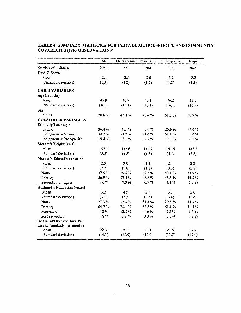
TABLE 4: SUMMARY STATISTICS FOR INDIVIDUAL, HOUSEHOLD, AND COMMUNITYCOVARIATES (2963 OBSERVATIONS)

All Chimaltenango TotonicapAn Suchitepiquez Jalapa

Number of Children 2963 727 784 853 862HI/A Z-Score

Mean -2.4 -2.5 -3.0 -1.9 -2.2(Standard deviation) (1.3) (1.2) (1.2) (1.2) (1.3)

CHILD VARIABLESAge (months)

Mean 45.9 46.7 45.1 46.2 45.5(Standard deviation) (16.1) (15.8) (16.1) (16.1) (16.3)

SexMales 50.0 % 45.8 % 48.4 % 51.1 % 50.9 %

HOUSEHOLD VARIABLESEthnicity/Language

Ladino 36.4 % 8.1 % 0.9 % 26.6 % 99.0 %Indigenous & Spanish 34.2 % 53.2 % 21.4 % 61.1 % 1.0 %Indigenous & No Spanish 29.4 % 38.7% 77.7 % 12.3 % 0.0 %

Mother's Height (cms)Mean 147.1 146.6 144.7 147.6 148.8(Standard deviation) (5.5) (4.8) (4.8) (5.5) (5.8)

Mother's Education (years)Mean 2.3 3.0 1.3 2.4 2.3(Standard deviation) (2.7) (2.8) (1.8) (3.0) (2.8)

None 37.5 % 19.6 % 49.5 % 42.1 % 38.0 %Primary 56.9 % 73.1% 48.8 % 48.8 % 56.8 %Secondary or higher 5.6 % 7.3 % 0.7 % 8.4 % 5.2 %

Husband's Education (years)Mean 3.2 4.5 2.5 3.2 2.6(Standard deviation) (3.1) (3.3) (2.5) (3.4) (2.8)

None 27.3 % 12.8 % 31.4% 29.5 % 34.3 %Primary 64.7 % 73.1 % 63.8 % 61.1 % 61.5 %Secondary 7.2% 12.8 % 4.6 % 8.3 % 3.3 %Post-secondary 0.8 % 1.3 % 0.0 % 1.1 % 0.9 %

Household Expenditure PerCapita (quetzals per month)

Mean 22.3 20.1 20.1 23.8 24.4(Standard deviation) (14.1) (12.0) (12.0) (13.7) (17.0)

36

(Table 4 continuedfrom previous page)All Chimaltenango Totonicapin SuchitepEquez Jalapa

COMMUNITY VARIABLESPublic Health Infrastructure% hhs with tap water insidea

Mean 0.04 0.02 0.001 0.15 0.01(Standard deviation) (0.11) (0.03) (0.01) (0.19) (0.02)

% hhs with toilet insideaMean 0.09 0.09 0.01 0.16 0.08(Standard deviation) (0.16) (0.12) (0.02) (0.23) (0.15)

Public dumpsite 8.3 °% 11.5 % 6.1 % 10.5 % 5.1 %

Modernization% hhs with TV'

Mean 0.33 0.45 0.25 0.33 0.27(Standard deviation) (0.24) (0.20) (0.18) (0.27) (0.26)

% literate women'Mean 0.73 0.89 0.59 0.72 0.76(Standard deviation) (0.193) (0.08) (0.17) (0.18) (0.19)

Economic StructurePaved road 6.6% 0.0% 13.9% 13.1 % 0.0%Commercial farms/Plantations 59.3 % 49.8 % 0.0 % 92.3 % 81.8 %Distance to nearest market (kms)

Mean 7.8 6.6 3.1 8.5 12.9(Standard deviation) (9.6i) (4.5) (2.9) (12.3) (12.4)

Total populationMean 2,587 2,708 3,008 2,587 2,046(Standard deviation) (2,120) (2,563) (1,219) (2,293) (2,260)

Bank/Rural cooperative 51.6 % 68.8 % 24.4 % 32.1% 77.9 %

Food Prices (quetzals/ounce)Rice

Mean 1.8 1.9 1.7 1.7 1.8(Standard deviation) (0.,2) (0.2) (0.2) (0.2) (0.2)

BeansMean 1.9 1.8 2.2 2.1 1.4(Standard deviation) (0.5) (0.5) (0.4) (0.4) (0.3)

CornMean 0.:5 0.4 0.6 0.6 0.5(Standard deviation) (0.1) (0.1) (0.1) (0.1) (0.1)

SugarMean 1.4 1.4 1.4 1.4 1.4(Standard deviation) (0.07) (0.06) (0.03) (0.09) (0.05)

SaltMean 0.4 0.4 0.3 0.4 0.4(Standard deviation) (0.(9) (0.08) (0.08) (0.09) (0.07)

37

(Table 4 continuedform previous page)All Chimaltenango Totonicapan Suchitepequez Jalapa

Ecological CharacteristicsAltitude (meters)b

Mean 1,570.8 2,086.7 2,593.3 410.0 1,193.3(Standard deviation) (885.3) (294.3) (303.5) (178.5) (300.5)

Health Care ServicesPrivate HCFC in the community 50.5 % 47.6 % 79.4 % 49.1 % 31.4%Government HCFd in community 37.7 % 49.5 % 29.0 % 48.4 % 22.8 %Number of doctors within 20 kms

Mean 1.52 1.00 0.73 1.53 2.80(Standard deviation) (1.75) (1.13) (0.96) (1.36) (2.48)

a From individual questionnaire.b Altitude of the municipality capital.'Hospital, clinic and pharmacy.d Health center, health post and IGSS clinic.

38

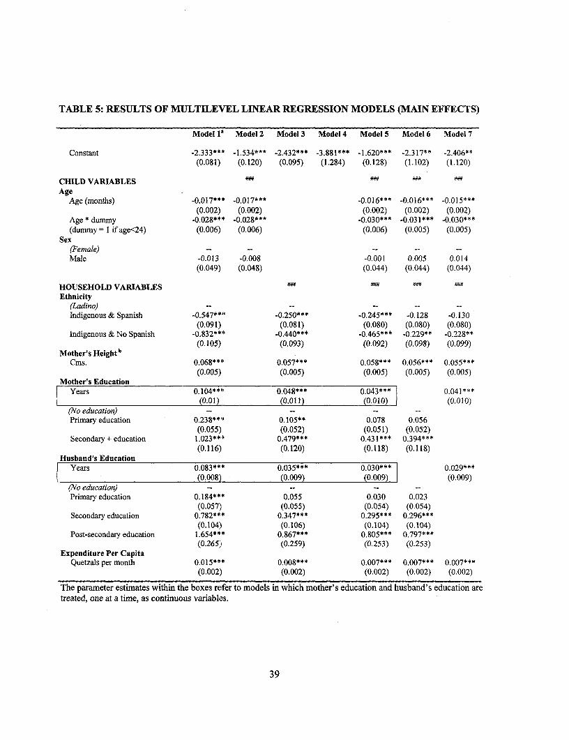
TABLE 5: RESULTS OF MULTILEVEL LINEAR REGRESSION MODELS (MAIN EFFECTS)

Model 11 Model 2 Model 3 Model 4 Model 5 Model 6 Model 7

Constant -2.333*** -1.534*** -2.432*** -3.881*** -1.620*** -2.317** -2.406**(0.081) (0.120) (0.095) (1.284) (0.128) (1.102) (1.120)

CHILD VARIABLES :.# #:#

AgeAge (months) -0.017*** -0.017*** -0.016*** -0.016*** -0.015***

(0.002) (0.002) (0.002) (0.002) (0.002)Age * dummy -0.028*** -0.028*** -0.030*** -0.031*** -0.030***(dummy = I if age<24) (0.006) (0.006) (0.006) (0.005) (0.005)

Sex(Female) -- -- -- -- --Male -0.013 -0.008 -0.001 0.005 0.014

(0.049) (0.048) (0.044) (0.044) (0.044)

HOUSEHOLD VARIABLES a

Ethnicity(Ladino) -- --

Indigenous & Spanish -0.547**'O -0.250*** -0.245*** -0.128 -0.130(0.091) (0.081) (0.080) (0.080) (0.080)

Indigenous & No Spanish -0.832**F -0.440*** -0.465*** -0.229** -0.228**(0.105) (0.093) (0.092) (0.098) (0.099)

Mother's HeightbCms. 0.068**4' 0.057*** 0.058*** 0.056*** 0.055***

(0.005) (0.005) (0.005) (0.005) (0.005)Mother's Education

Years 0.104***C 0.048*** 0.043*** 0.041***(0.01) (0.011) (0.010) (0.010)

(No education) -- -- -- --

Primary education 0.238**' 0.105** 0.078 0.056(0.055) (0.052) (0.051) (0.052)

Secondary + education 1.023*** 0.479*** 0.431*** 0.394***(0.116) (0.120) (0.118) (0.118)

Husband's EducationYears 0.083*** 0.035*** 0.030*** 0.029***

(0.008) (0.009) (0.009)l (0.009)(No education) -- -- -- --

Primary education 0.184*** 0.055 0.030 0.023(0.057), (0.055) (0.054) (0.054)

Secondary education 0.782*** 0.347*** 0.295*** 0.296***(0.104) (0.106) (0.104) (0.104)

Post-secondary education 1.654*** 0.867*** 0.805*** 0.797***(0.265) (0.259) (0.253) (0.253)

Expenditure Per CapitaQuetzals per month 0.015*** 0.008*** 0.007*** 0.007*** 0.007***

(0.002) (0.002) (0.002) (0.002) (0.002)

The parameter estimates within the boxes refer to models in which mother's education and husband's education aretreated, one at a time, as continuous variables.

39

(Table 5 continuedfrom previous page)Model 1 Model 2 Model 3 Model 4 Model S Model 6 Model 7

COMMUNITY VARIABLES ". .::

Public Health Infrastructure NO

%hhswithtapwaterinside 2.385*** 1.813*** 1.232** 1.151**(0.589) (0.584) (0.499) (0.507)

% hhs with toilet inside 1.993*** -1.559** -1.466*** -1.352***(0.418) (0.574) (0.494) (0.501)

(No Public dumpsite) -- -- -- --

Public dumpsite in the community 0.385 0.343** 0.310** 0.318**(0.267) (0.170) (0.145) (0.147)

Modernization ON #.

% hhs with TV 1.268*** 1.259*** 0.769*** 0.748***(0.281) (0.267) (0.229) (0.233)

%literatewomen 1.671*** 0.712** 0.464 0.330(0.368) (0.334) (0.289) (0.290)

Economic Structure(No Paved road) --

Paved road -0.018 -0.050 0.037 0.029(0.324) (0.163) (0.141) (0.143)

Distance to the nearest market -0.011 -0.012** 0.005 0.004(0.008) (0.006) (0.005) (0.005)

(No Commercialfarms/Plantations) -- -- -- --

Commercial farms/Plantations 0.679*** 0.174* 0.103 0.113(0.138) (0.101) (0.095) (0.097)

Total populationb -0.012 -0.090*** -0.055*** -0.057***(0.038) (0.025) (0.021) (0.022)

(No Bank/Rural cooperative) -- -- -- --

Bank/Rural cooperative 0.323** -0.055 -0.056 -0.058(0.157) (0.087) (0.074) (0.075)

Food Prices (quetzals/ounce)Rice -0.167 0.110 -0.018 0.000

(0.328) (0.185) (0.159) (0.162)Beans -0.040 0.019 0.132 0.137

(0.163) (0.094) (0.085) (0.086)Corn -0.020 0.749 0.321 0.341

(0.017) (0.459) (0.403) (0.410)Sugar 2.050 -0.393 -0.509 -0.473

(1.130) (0.936) (0.796) (0.809)Salt 1.879** 0.866 0.848 0.789

(0.922) (0.642) (0.550) (0.560)Ecological Characteristics U UN U

(Altitude < 1500 meters) -- - -- --

Altitude 1500 - 2500 meters -0.517*** -0.310*** -0.273*** -0.291***(0.150) (0.114) (0.097) (0.099)

Altitude > 2500 -0.920*** .0.608*** -0.453*** -0.466***(0.183) (0.142) (0.127) (0.128)

Health Care Services(No Private HCF in community) -- -- -- --

Private HCF in commnunity 0.0003 0.016 -0.018 -0.022(0.163) (0.110) (0.093) (0.095)

(No Gover. HCF in community) -- -- -- --

Government HCF in community 0.356** 0.236** 0.177** 0. 167*(0.159) (0.101) (0.086) (0.085)

Number of doctors within 20 kms 0.125*** 0.108*** 0.059** 0.052**(0.044) (0.029) (0.026) (0.026)

Omitted categories are shown in parentheses.*P-Value < 0.1; ** P-Value < 0.05; *** P-Value < 0.01." Jointly significant at the 5% level; " Jointly significant at the 1% level.a Models with only one variable at a time. b Mean-centered.

40

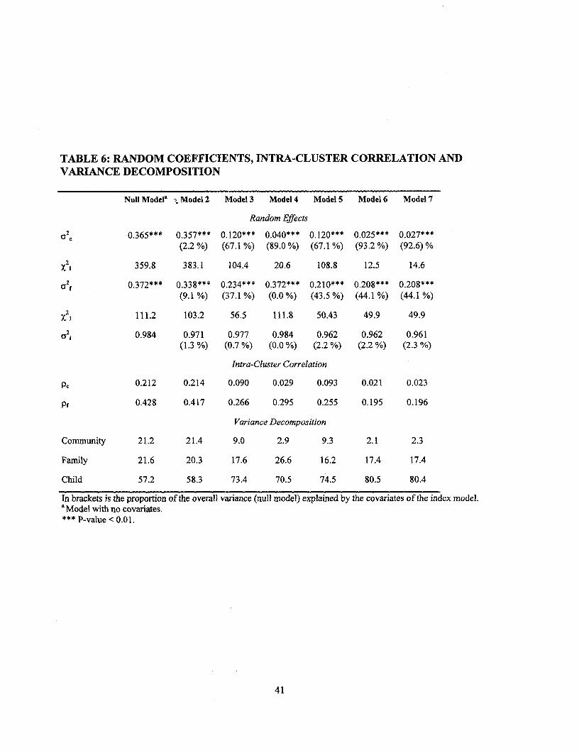
TABLE 6: RANDOM COEFFICIENTS, INTRA-CLUSTER CORRELATION ANDVARIANCE DECOMPOSITION

Null Model| Model 2 Model 3 Model 4 Model 5 Model 6 Model 7

Random Effects

cr c 0.365*** 0.357*** 0.120*** 0.040*** 0.120*** 0.025*** 0.027***(2.2 %) (67.1 %) (89.0 %i) (67.1 %) (93.2 %) (92.6) %

x 21 359.8 383.1 104.4 20.6 108.8 12.5 14.6

2 0.372*** 0.338*** 0.234*** 0.372*** 0.210*** 0.208*** 0.208***(9.1 %) (37.1 %) (0.0 %) (43.5 %) (44.1 %) (44.1 %)

X21 111.2 103.2 56.5 111.8 50.43 49.9 49.9

a2i 0.984 0.971 0.977 0.984 0.962 0.962 0.961(1.3 %) (0.7 %) (0.0 %) (2.2%) (2.2 %) (2.3 %)

Intra-Cluster Correlation

PC 0.212 0.214 0.090 0.029 0.093 0.021 0.023

pf 0.428 0.417 0.266 0.295 0.255 0.195 0.196

Variance Decomposition

Community 21.2 21.4 9.0 2.9 9.3 2.1 2.3

Family 21.6 20.3 17.6 26.6 16.2 17.4 17.4

Child 57.2 58.3 73.4 70.5 74.5 80.5 80.4

In brackets is the proportion of the overall variance (null model) explained by the covariates of the index model.a Model with no covariates.*** P-value < 0.01.

41

FIGURE 3: BOX-PLOTS OF COMMUNITY-LEVEL RESIDUALS FROM REDUCED-FORM MODELS*

@ Community-Level Residuals1.25

.X2127

T

-1.25 -Null Model 2 Model 3 Model 4 Model 5 Model 6 Model 7

*Community-level residuals are defined as predicted minus observed outcomes

42

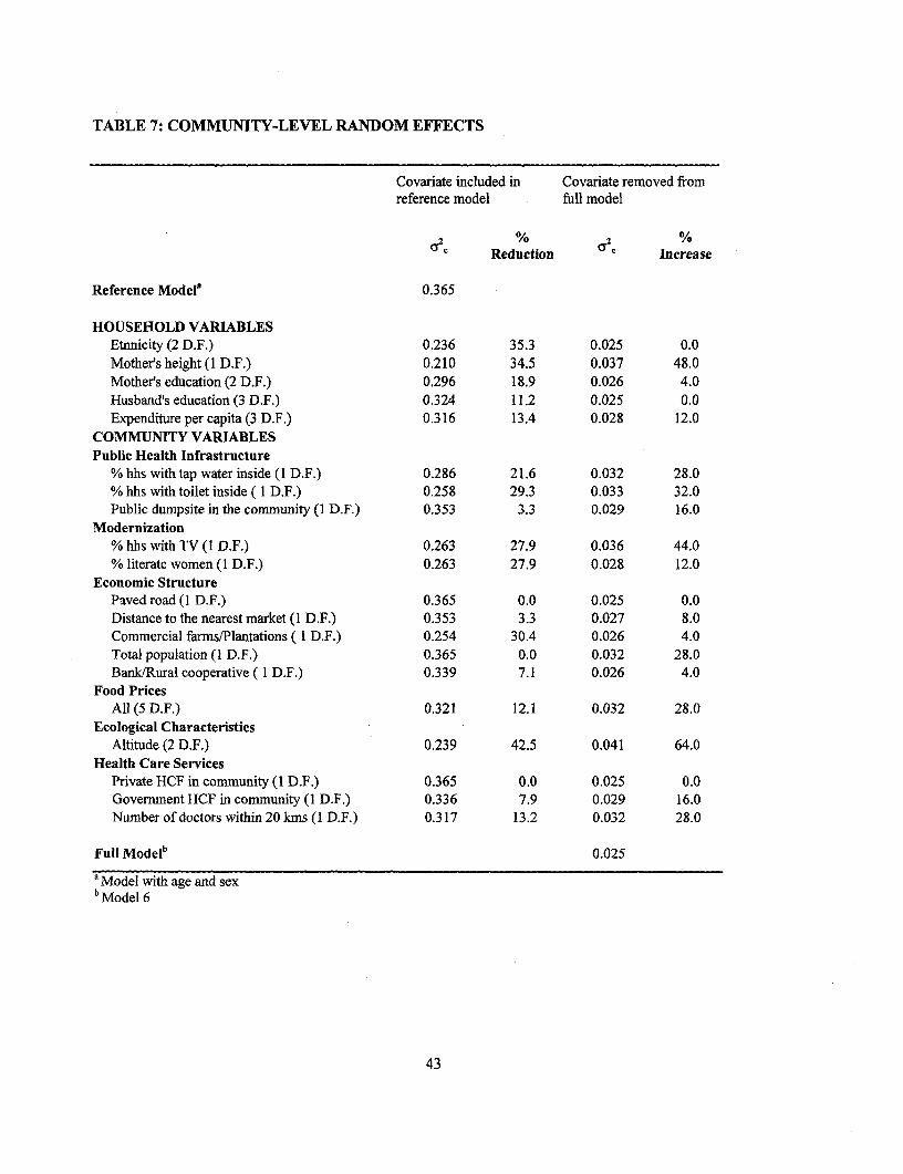
TABLE 7: COMMUNITY-LEVEL RANDOM EFFECTS

Covariate included in Covariate removed fromreference model full model

g % 2 %

Reduction 0 C Increase

Reference Model' 0.365

HOUSEHOLD VARIABLESEtnnicity (2 D.F.) 0.236 35.3 0.025 0.0Mother's height (I D.F.) 0.210 34.5 0.037 48.0Mother's education (2 D.F.) 0.296 18.9 0.026 4.0Husband's education (3 D.F.) 0.324 11.2 0.025 0.0Expenditure per capita (3 D.F.) 0.316 13.4 0.028 12.0

COMMUNITY VARIABLESPublic Health Infrastructure

% hhs with tap water inside (1 D.F.) 0.286 21.6 0.032 28.0% hhs with toilet inside ( I D.F.) 0.258 29.3 0.033 32.0Public dumpsite in the community (I D.F.) 0.353 3.3 0.029 16.0

Modernization% hhs with TV (1 D.F.) 0.263 27.9 0.036 44.0% literate women (I D.F.) 0.263 27.9 0.028 12.0

Economic StructurePaved road (1 D.F.) 0.365 0.0 0.025 0.0Distance to the nearest market (I D.F.) 0.353 3.3 0.027 8.0Commercial farms/Plantations ( 1 D.F.) 0.254 30.4 0.026 4.0Total population (1 D.F.) 0.365 0.0 0.032 28.0Bank/Rural cooperative ( I D.F.) 0.339 7.1 0.026 4.0

Food PricesAll (5 D.F.) 0.321 12.1 0.032 28.0

Ecological CharacteristicsAltitude (2 D.F.) 0.239 42.5 0.041 64.0

Health Care ServicesPrivate HCF in community (I D.F.) 0.365 0.0 0.025 0.0Government HCF in community (1 D.F.) 0.336 7.9 0.029 16.0Number of doctors within 20 kms (I D.F.) 0.317 13.2 0.032 28.0

Full Modelb 0.025

' Model with age and sexb Model 6

43

TABLE 8: INTRA-FAMELY CORRELATION*

Covariate included in null model Covariate removed from fullmodel

Pf % Pf %Reduction Increase

Reference Modela 0.338

HOUSEHOLD VARIABLESEthnicity (2 D.F.) 0.320 5.3 0.212 8.7Mother's height (I D.F.) 0.254 24.9 0.264 35.4Mother's education (2 D.F.) 0.309 8.6 0.213 9.2Husband's education (3 D.F.) 0.296 12.4 0.215 10.3Expenditure per capita (3 D.F.) 0.309 8.6 0.215 10.3

Full Modelb 0.195

* pf = (ay2 + (O2f )/(U2c + 2f + ( 2 )

a Model with age and sexb Model 6

44

TABLE 9: RANDOM-COEFFICIENTS MODELS: LIKELIHOOD-RATIO TESTS FORRANDOM EFFECTS OF EDUCATION AND EXPENDITURE

Mother's Education Husband's Education Expenditure Per Capita

X22 0.00 4.64 2.10

P-Value 1.000 0.098 0.350

45

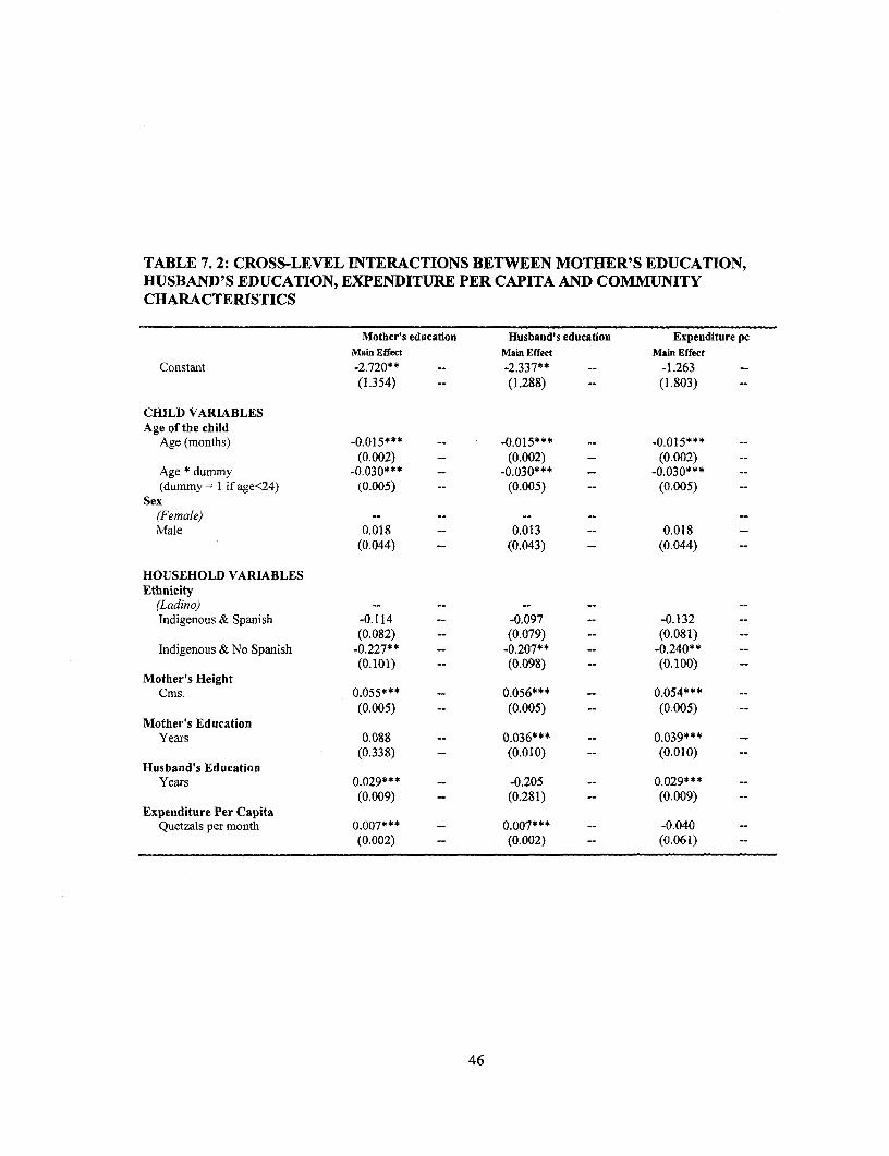
TABLE 7.2: CROSS-LEVEL INTERACTIONS BETWEEN MOTHER'S EDUCATION,HUSBAND'S EDUCATION, EXPENDITURE PER CAPITA AND COMMUNITYCHARACTERISTICS

Mother's education Husband's education Expenditure pcMain Effect Main Effect Main Effect

Constant -2.720** -- -2.337** -- -1.263 --

(1.354) -- (1.288) (1.803)

CHILD VARIABLESAge of the child

Age (months) -0.015*** -- -0.015*** -- -0.015***(0.002) -- (0.002) (0.002) --

Age * dummy -0.030*** -0.030*** -0.030*** --

(dummy= I if age<24) (0.005) -- (0.005) (0.005)Sex

(Female) -- -- - -- --

Male 0.018 -- 0.013 -- 0.018 --

(0.044) -- (0.043) -- (0.044) --

HOUSEHOLD VARIABLESEthnicity

(Ladino) -- -- -- -- --

Indigenous & Spanish -0.114 -- -0.097 -- -0.132 --

(0.082) -- (0.079) -- (0.081)Indigenous & No Spanish -0.227** -- -0.207** -- -0.240** --

(0.101) (0.098) -- (0.100) --

Mother's HeightCms. 0.055*** 0.056*** -- 0.054*** --

(0.005) -- (0.005) -- (0.005) --

Mother's EducationYears 0.088 -- 0.036*** -- 0.039*** --

(0.338) -- (0.010) -- (0.010) --

Husband's EducationYears 0.029*** -- -0.205 -- 0.029*** --

(0.009) -- (0.281) -- (0.009) --

Expenditure Per CapitaQuetzals per month 0.007*** -- 0.007*** -- -0.040 --

(0.002) -- (0.002) (0.061) --

46

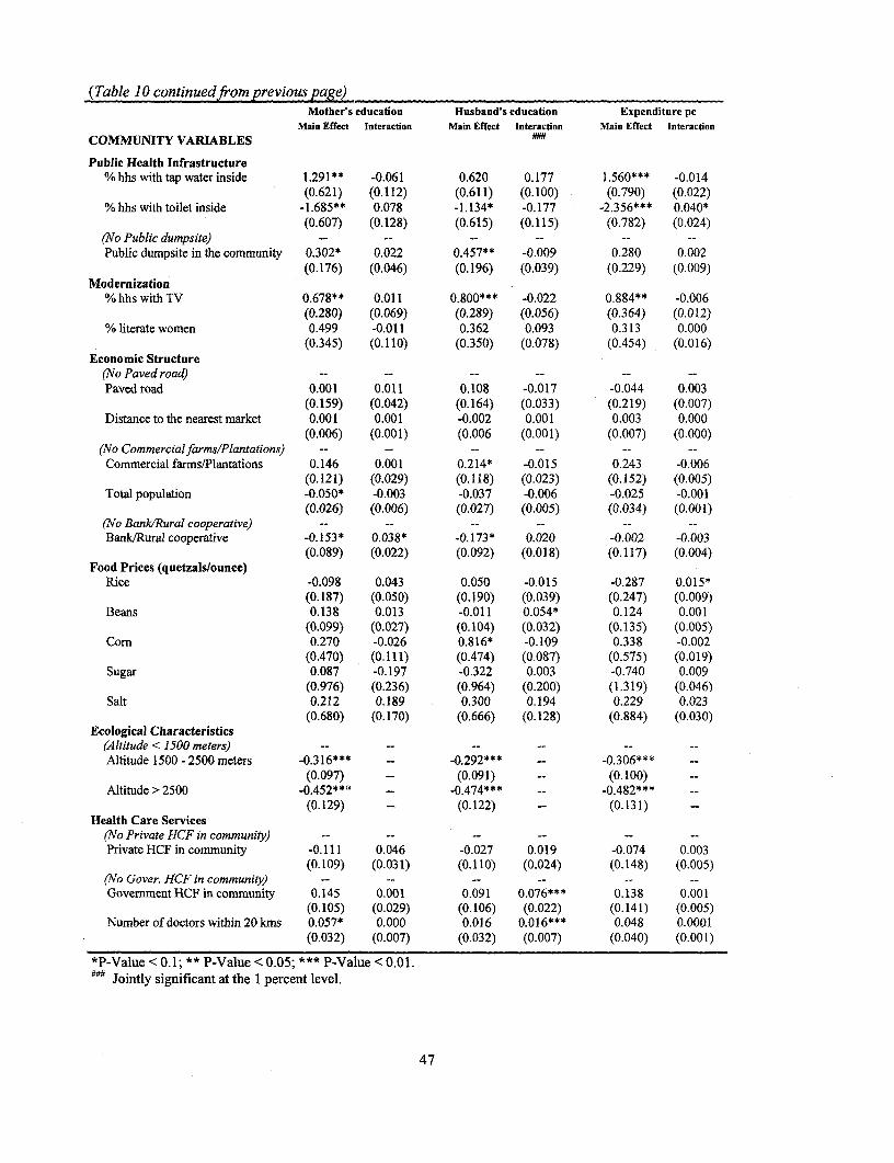
(Table IO continuedfrom previous page)Mother's education Husband's education Expenditure pc

Main Effect Interaction Main Effect Interaction Main Effect InteractionCOMMUNITY VARIABLES

Public Health Infrastructure% hhs with tap water inside 1.291** -0.061 0.620 0.177 1.560*** -0.014

(0.621) (0.112) (0.611) (0.100) (0.790) (0.022)% hhs with toilet inside -1.685** 0.078 -1.134* -0.177 -2.356*** 0.040*

(0.607) (0.128) (0.615) (0.115) (0.782) (0.024)(No Public dumpsite) -- -- -- -- -- --Public dumpsite in the community 0.302* 0.022 0.457** -0.009 0.280 0.002

(0.176) (0.046) (0.196) (0.039) (0.229) (0.009)Modernization

% hhs with TV 0.678** 0.011 0.800*** -0.022 0.884** -0.006(0.280) (0.069) (0.289) (0.056) (0.364) (0.012)

% literate women 0.499 -0.011 0.362 0.093 0.313 0.000(0.345) (0.110) (0.350) (0.078) (0.454) (0.016)

Economic Structure(No Paved road) -- -- -- -- -- --

Paved road 0.001 0.011 0.108 -0.017 -0.044 0.003(0.159) (0.042) (0.164) (0.033) (0.219) (0.007)

Distance to the nearest market 0.001 0.001 -0.002 0.001 0.003 0.000(0.006) (0.001) (0.006 (0.001) (0.007) (0.000)

(No Commercialfarms/Plantations) -- -- -- -- -- --Commercial farms/Plantations 0.146 0.001 0.214* -0.015 0.243 -0.006

(0.121) (0.029) (0.118) (0.023) (0.152) (0.005)Total population -0.050* -0.003 -0.037 -0.006 -0.025 -0.001

(0.026) (0.006) (0.027) (0.005) (0.034) (0.001)(No BankWRural cooperative) -- -- -- -- -- --Bank/Rural cooperative -0.153* 0.038* -0.173* 0.020 -0.002 -0.003

(0.089) (0.022) (0.092) (0.018) (0.117) (0.004)Food Prices (quetzalslounce)

Rice -0.098 0.043 0.050 -0.015 -0.287 0.015*(0.187) (0.050) (0.190) (0.039) (0.247) (0.009)

Beans 0.138 0.013 -0.011 0.054* 0.124 0.001(0.099) (0.027) (0.104) (0.032) (0.135) (0.005)

Corn 0.270 -0.026 0.816* -0.109 0.338 -0.002(0.470) (0.111) (0.474) (0.087) (0.575) (0.019)

Sugar 0.087 -0.197 -0.322 0.003 -0.740 0.009(0.976) (0.236) (0.964) (0.200) (1.319) (0.046)

Salt 0.212 0.189 0.300 0.194 0.229 0.023(0.680) (0.170) (0.666) (0.128) (0.884) (0.030)

Ecological Characteristics(Altitude < 1500 meters) -- -- -- -- -- --

Altitude 1500 -2500 meters -0.316**" - -0.292*** -0.306*** --

(0.097) - (0.091) (0.100)Altitude > 2500 -0.452**t -_0.474*** -0.482*** --

(0.129) - (0.122) -- (0.131)Health Care Services

(No Private HCF in community) -- -- -- -- -- --

Private HCF in community -0.111 0.046 -0.027 0.019 -0.074 0.003(0.109) (0.031) (0.110) (0.024) (0.148) (0.005)

(No Gover. HCF in community) - -- -- -- -- --Govemment HCF in community 0.145 0.001 0.091 0.076*** 0.138 0.001

(0.105) (0.029) (0.106) (0.022) (0.141) (0.005)Number of doctors within 20 kms 0.057* 0.000 0.016 0.016*** 0.048 0.0001

(0.032) (0.007) (0.032) (0.007) (0.040) (0.001)

*P-Value < 0.1; ** P-Value < 0.05; *** P-Value < 0.01.#44 Jointly significant at the 1 percent level.

47

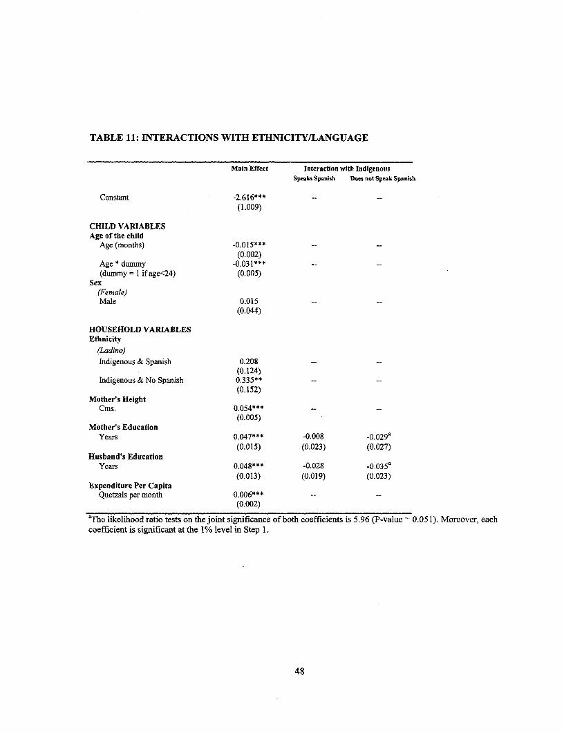
TABLE 11: INTERACTIONS WITH ETHNICITY/LANGUAGE

Main Effect Interaction with IndigenousSpeaks Spanish Does not Speak Spanish

Constant -2.616***(1.009)

CHILD VARIABLESAge of the child

Age (months) -0.015*** --(0.002)

Age * dummy -0.031*** -- --

(dummy = I if age<24) (0.005)Sex

(Female)Male 0.015 -- --

(0.044)

HOUSEHOLD VARIABLESEthnicity

(Ladino)Indigenous & Spanish 0.208 -- --

(0.124)Indigenous & No Spanish 0.335** --

(0.152)Mother's Height

Cms. 0.054*** --

(0.005)Mother's Education

Years 0.047*** -0.008 -0.029a(0.015) (0.023) (0.027)

Husband's EducationYears 0.048*** -0.028 -0.035a

(0.013) (0.019) (0.023)Expenditure Per Capita

Quetzals per month 0.006*** -- --

(0.002)

aThe likelihood ratio tests on the joint significance of both coefficients is 5.96 (P-value = 0.051). Moreover, eachcoefficient is significant at the 1% level in Step 1.

48

(Table 1] continuedfrom previous page)Main Eflect Interaction with Indigenous

Speaks Spanish Does not Speak Spanish

COMMUNITY VARIABLESPublic Health Infrastructure

% hhs with tap water inside 1.521* *-(0.468)

% hhs with toilet inside -1.996*** --

(0.478)(No Public dumpsite)Public dumpsite in the community 0.348***

(0.13 3)Modernization

% hhs with TV 0.832*** --

(0.209)% literate women 0.216 -- --

(0.265)Economic Structure

(No Paved road)Paved road 0.022 --

(0.130)Distance to the nearest market 0.005 -- --

(0.004)(No Commercial farms/Plantations)Commercial farms/Plantations 0.132 -- --

(0.087)Total population -0.063*** -- --

(0.019)(No Bank/Rural cooperative)Bank/Rural cooperative 0.010 -- --

(0.069)Food Prices (quetzals/ounce)

Rice 0.017 -- --

(0.145)Beans 0.13,0 -- --

(0.079)Corn 0.265 -- --

(0.372)Sugar -0.505

(0.733)Salt 0.991

(0.5'19)Ecological Characteristics

(Altitude < 1500 meters)Altitude 1500 - 2500 meters -0.359*** -- --

(0.0!90)Altitude > 2500 -0.51 *** -- --

(0.116)Health Care Services

(No Private HCF in community)Private HCF in community -0.035*** -- --

(0.085)(No Gover. HCF in community)Government HCF in community 0.389*** -0.181 -0.389***

(0.126) (0.138) (0.153)Number of doctors within 20 kms 0.094 -0.076 -0. 155***

(0.029) (0.048) (0.056)

*P-Value < 0.1; ** P-Value < 0.05; *** P-Value < 0.01.

49

Policy Research Working Paper Series

ContactTitle Author Date for paper

WPS2174 Prospective Deficits and the Asian Craig Burnside September 1999 E. KhineCurrency Crisis Martin Eichenbaum 37471

Sergio Rebelo

WPS2175 Sector Growth and the Dual Eccinomy Niels-Hugh Blunch September 1999 H. VargasModel: Evidence from Cote d'voire, Dorte Verner 37871Ghana, and Zimbabwe

WPS2176 Fiscal Risks and the Quality of Hana Polackova Brixi September 1999 A. PantonFiscal Adjustment in Hungary Anita Papp 85433

Allen Schick

WPS2177 Fiscal Adjustment and Contingent Hana Polackova Brixi September 1999 A. PantonGovernment Liabilities: Case Studies Hafez Ghanem 85433Of the Czech Republic and Macedonia Roumeen Islam

WPS2178 Nonfarm Income, Inequality, and Land Richard H. Adams Jr. September 1999 M. Coleridge-TaylorIn Rural Egypt 33704

WPS2179 How Child Labor and Child Schooling Ranjan Ray September 1999 M. MasonInteract with Adult Labor 30809

WPS2180 Regulating Privatized Infrastructures Ofelia Betancor September 1999 G. Chenet-Smithand Airport Services Robert Rendeiro 36370

WPS2181 Privatization and Regulation of the Lourdes Trujillo September 1999 G. Chenet-SmithSeaport Industry Gustavo Nombela 36370

WPS2182 The Integration of Transition Constantine Michalopoulos September 1999 L. TabadaEconomies into the World Trading 36896System

WPS2183 Market Discipline and Financial Asli Demirguc-Kunt September 1999 K. LabrieSafety Net Design Harry Huizinga 31001

WPS2184 Financial Services and the WcrId Aaditya Mattoo September 1999 L. TabadaTrade Organization: Liberalization 36896Commitments of the Developingand Transition Economies

WPS2185 Financial Sector Inefficiencies and Pierre-Richard Agenor September 1999 T. ShielCoordination Failures: Implications Joshua Aizenman 36317for Crisis Management

WPS2186 Contagion, Bank Lending Spreads, Pierre-Richard Agenor September 1999 T. Shieland Output Fluctuations Joshua Aizenman 36317

Alexander Hoffmaister

Policy Research Working Paper Series

ContactTitle Author Date for paper

WPS2187 Who Determines Mexican Trade Jean-Marie Grether September 1999 L. TabadaPolicy? Jaime de Melo 36896

WPS2188 Financial Liberalization and the Pedro Alba September 1999 R. VoCapital Account: Thailand, 1988-97 Leonardo Hernandez 33722

Daniela Klingebiel

WPS2189 Alternative Frameworks for Stijn Claessens September 1 9Y9 R. VoProviding Financial Services Daniela Klingebiel 33722

WPS2190 The Credit Channel at Work: Lessons Giovanni Ferri September 1999 K. Labriefrom the Republic of Korea's Financial Tae Soo Kang 31001Crisis

WPS2191 Can No Antitrust Policy Be Better Aaditya Mattoo September 1999 L. TabadaThan Some Antitrust Policy? 36896

WPS2192 Districts, Spillovers, and Government Reza Baqir September 1999 S. DevadasOverspending 87891