statistical proces control - david howard

8/3/2019 Statistical Proces Control - David Howard

http://slidepdf.com/reader/full/statistical-proces-control-david-howard 1/17

THE BASICS OF

STATISTICAL PROCESS CONTROL& PROCESS BEHAVIOUR CHARTING

A User’s Guide to SPC

By David Howard

Management-NewStyle



The Basics of Control Charting

2

"...Shewhart perceived that control limits must serve industry in action. A. process, even instatistical control, wavers. Control limits can thus not be associated with any exact

probability of looking for trouble (an assignable cause) when there is none, nor with failure tolook for trouble when an assignable cause does exist. It was for such reasons that he used 3-sigma control limits. Experience of over 50 years shows how right he was."

W Edwards Deming (1900-1993)

Management-NewStyle is grateful to Mal Owen for permissionto draw upon examples and illustrations from Chapter 5 of his book

SPC and Business Improvement in preparing this booklet.




3

Contents

1 Introduction 5

2 Histograms & Charts 5

3 Common and Special Causes 6

4 Control Limits 7

5 Using SPC to Drive Improvement 9

6 Collecting Data 10

7 Basis for Control Chart Limits 11

8 Shewhart or Otherwise? 13

9 Points to Note 14

10 Key Words 14

Appendix

Calculations 16Constants 16References 17




4

Figure 1 - W A Shewhart (1891-1967)

“How much variation should we leave to chance?”

Figure 2 - The first control chart – 1924

Figure 3 - Example of a FlowMap SPC-Plus control chart – 2003




5

1. INTRODUCTION

Statistical Process Control (SPC) charts offer users the chance to monitor the veryheartbeat of their processes. By collecting data they can predict performance. Taking

sample readings from a process seems straightforward. Of does it? Look moreclosely. Do we understand our process fully?

In manufacturing areas we probably do. In non-manufacturing areas we may be lessconfident. And who collects the data? What sample size is required? How often aresamples taken? These are vital questions to those intending to daily use the controlchart with a view to improving process performance, particularly in non-manufacturing, or service, areas where the techniques are new.

The control chart has been with us since 1924. It has been tried and proven, andaccepted as a highly effective tool in improving processes. In view of the fact that

there is currently renewed interest in Shewhart's work, it is important to considerhow the control limits were originally set up.

However, at the end of the day, it is the logic and rules of collecting data andinterpreting the pattern of points on the chart that is the important issue inunderstanding process behaviour and the discovery of insights for processimprovement.

2. HISTOGRAMS & CHARTS

Figure 4 shows a typical set of readings obtained by collecting samples from aprocess. Control charting requires the mean of each sample to be used, rather thanthe individuals. Figure 4 also shows the calculated values of the mean X and rangeR.

Figure 4 – Presentation of sample data

The first stage in constructing a control chart for X requires X , the mean, to be plottedagainst time as shown in Figure 5.




6

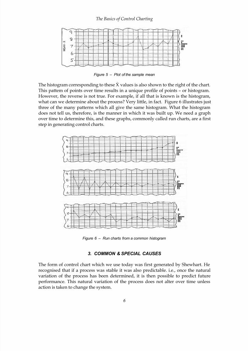
Figure 5 – Plot of the sample mean

The histogram corresponding to these X values is also shown to the right of the chart.This pattem of points over time results in a unique profile of points – or histogram.However, the reverse is not true. For example, if all that is known is the histogram,what can we determine about the process? Very little, in fact. Figure 6 illustrates justthree of the many patterns which all give the same histogram. What the histogramdoes not tell us, therefore, is the manner in which it was built up. We need a graphover time to determine this, and these graphs, commonly called run charts, are a first

step in generating control charts.

Figure 6 – Run charts from a common histogram

3. COMMON & SPECIAL CAUSES

The form of control chart which we use today was first generated by Shewhart. Herecognised that if a process was stable it was also predictable. i.e., once the naturalvariation of the process has been determined, it is then possible to predict futureperformance. This natural variation of the process does not alter over time unlessaction is taken to change the system.




7

A process is defined as being stable if its natural variation is due to common causes.The process is then said to be under statistical control. If a process is unstable, that isbecause unusual factors are operating on the process. These factors, known as specialcauses, result in the process being out of statistical control. Shewhart recognised thatwe make mistakes at times, in that we take action when we should not do so.

Equally, we sometimes let things drift, assuming the process will right itself, when infact we should react at the first sign of trouble. Shewhart was therefore aiming todevise a rule which would be sensitive enough to pick up a special cause, but not sosensitive as to react to extremes in terms of common causes.

Take the figures plotted in Figure 5 as an example. It makes sense to use a centralvalue as a reference point. The best measure of central location is the mean value,that is the ‘average’ obtained by adding all one hundred readings and dividing thetotal by 100, giving:

733 / 100 = 7.33

In fact, this mean can be obtained much more directly. We already have the values ofthe 20 sample means. Hence the overall mean is given by the following calculation:

∑X / 20 = 146.6/20= 7.33

This mean of the sample means is known as the grand mean, or x (X double bar),thus:

x = 7.33

Figure 7 shows our run chart of X

values together with a line for x

conventionallydrawn as a broken line and often called the central line. The question is now wheredo we draw lines on the chart which will sensibly indicate the presence of specialcauses?

Figure 7 – Run chart for X with central line

4. CONTROL LIMITS

If we draw lines too close to x as in Fig 6 then we will be reacting too often to pointswhich are really part of the system and not special causes. Fig 7 shows the reverse -lines set so far out that they will not pick up any change unless it is a major one andobvious. A balance between these two cases is required. Shewhart chose lines set at




8

three standard deviations away from x - commonly known as control limits. Whythree standard deviations? Because this number has been found to be economicallypractical in use over the past 75 years.It keeps a balance between over, and under,reaction to process behaviour patterns. Such limits represent pragmatically powerfulmarkers of change in process performance. The can reliably provide a predictivewarning of an onset of instability.

Figure 8 – Control chart for X

Figure 9 – Run chart with decision lines too near to X

There is a bit more to it than that, however, as you might expect, and the apparent

simplicity of this rule brings with it some controversy. The derivation of the controllimits has been a point of discussion on both sides of the Atlantic for over half acentury. This is because Shewhart's original thinking has been augmented by others.(In particular we would refer the reader to the work of Don Wheeler, in the US, listedon p 24.)

In order to complete the control chart for X , we now add a central line and upper andlower control limits (denoted by UCLx and LCLx ). This gives us the chart shown inFigure 10.

Figure 10 – Run chart with decision lines too far from X




9

Determining the position of the lines will involve some simple formulae whichdepend on whether we are looking at multiple of individual readings. The arithmeticsteps to calculate the limits are easy to master and summarised in the Appendix.

5. USING SPC TO DRIVE IMPROVEMENT

Whether charting variables or attributes the approach follows the same sequence: 1)Define the process; 2) Collect the data; 3) Set up the chart; 4) Plot the results; 5)Check on control, and 6) Adjust the process. Let us now consider each in turn. Inmanufacturing areas a process is easy to understand and define. In non-manufacturing areas it is less so. The processes tend to be more complex and moredifficult to specify clearly.

A definition of the process needs to be obtained, but it requires careful preparatorywork. Flow charting is a key tool in this definition. An additional problem is thatadministrative processes are much more people-orientated and as a result,

personalities and emotions are involved. (See the companion booklet The Basics of Deployment FlowCharting & Process Mapping for details of process mapping).

Process data for charting is collected by taking sample readings. Sampling, asopposed to 100% inspection, is not only easier, it is more representative and quicker.The sampling procedure will differ for variables and attributes. For variables,collecting the data involves issues of sample size, number of samples and theirfrequency. For attributes sampling is the exception, not the rule.Manufacturingexamples generally use samples with a size of 5. These are taken from the process atregular intervals and represented on the (X , R) chart. Figure 11 indicates how thedata may be collected and organised on a collection sheet ready to be recorded on acontrol chart.

Figure 11 – Collection and recording of sample data




10

In non-manufacturing, the use of a sample tends to be the exception. In practice it ismuch more likely that we are looking at single readings - one document, one salesfigure, one event. Single reading values are monitored using what we call (X, movingR) charts. However, there is a certain logic about the sequence in which control chartsare introduced.

There is a natural flow in progressing from sampled values to dealing withindividual values, and there is a danger of confusing the understanding if thissequence is changed. In starting with control charts it is therefore helpful to firstlyexplore (X , R) charts and then progress to (X, moving R) charts. If we are looking atprocessing times, for example, then five documents could be tagged first thing in themorning and subsequently the time when each document is completed would benoted. For financial data, for example sales figures, five results would be taken in ansuitable manner from the many figures which are available.

The ideal number of different samples needed to construct a chart with control limitsis generally 20. There is no reason why interim calculations of process limits could

not be carried out on fewer than 20 samples and then updated when 20 samples areavailable.

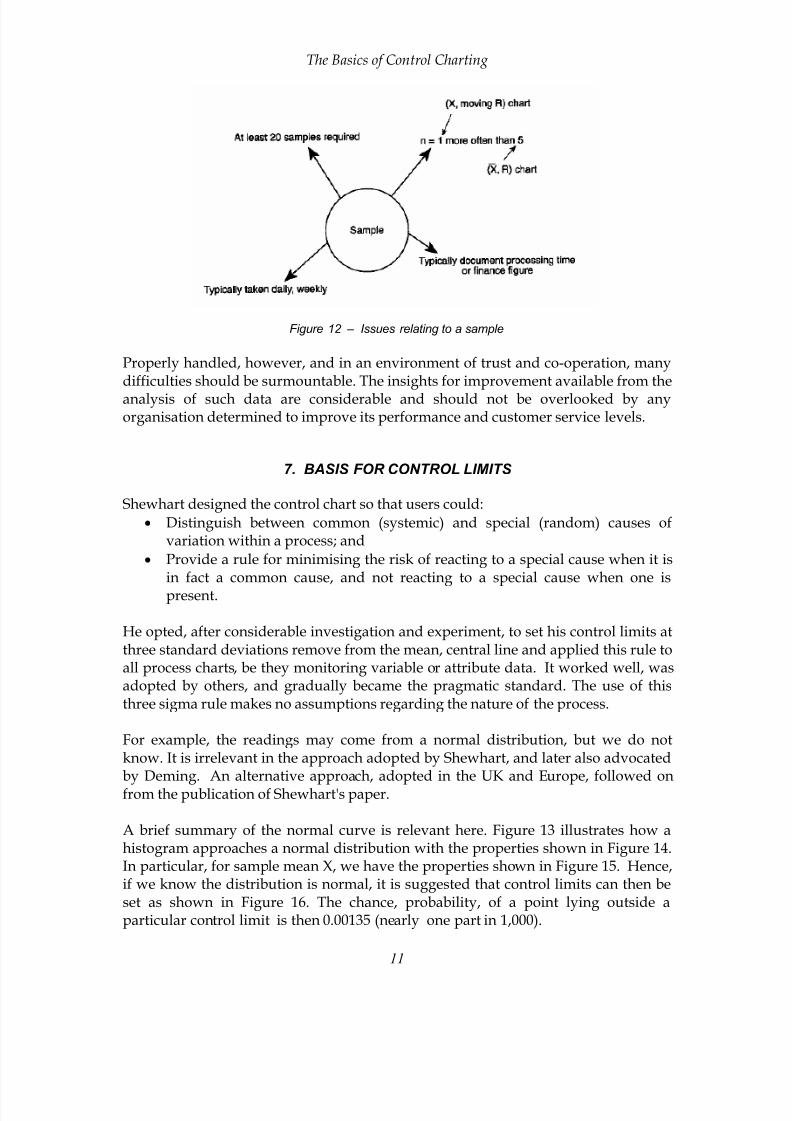
In administrative areas the frequency is typically daily, weekly, or even monthly. Judgement will dictate. The nature of the great majority of processes does not allowfor sampling at hourly intervals or less, as commonly applied in manufacturing. Oddexceptions may emerge. For example, response times to a computer programmecould be taken every 15 minutes. Figure 12 provides a summary of some of theissues associated with sampling.

6. COLLECTING THE DATA

Whatever the organisation, manufacturing or otherwise, personnel should beresponsible for monitoring their own processes. Hence, in the same way as operatorsin manufacturing industry collect data, their equivalents in non-manufacturing -clerical assistants, clerks, technical support staff, managers – should all collectsampled data for their administrative processes.

This may cause problems initially since it is a change from the tradition of looking fortrends in data or comparing the data of one period with another. Administrativepeople recognise that data has traditionally been collected in order to measure levels

of productivity, rather than the inherent capability of their processes.

There may be a natural reluctance to assist in an activity which may haverepercussions on their own employment. This is understandable but managementhas the duty to re-assure those who may be confused if process change is to beachieved by the informed analysis of available data with the intention ofimprovement action.




11

Figure 12 – Issues relating to a sample

Properly handled, however, and in an environment of trust and co-operation, manydifficulties should be surmountable. The insights for improvement available from theanalysis of such data are considerable and should not be overlooked by anyorganisation determined to improve its performance and customer service levels.

7. BASIS FOR CONTROL LIMITS

Shewhart designed the control chart so that users could:

• Distinguish between common (systemic) and special (random) causes ofvariation within a process; and

• Provide a rule for minimising the risk of reacting to a special cause when it isin fact a common cause, and not reacting to a special cause when one ispresent.

He opted, after considerable investigation and experiment, to set his control limits atthree standard deviations remove from the mean, central line and applied this rule toall process charts, be they monitoring variable or attribute data. It worked well, wasadopted by others, and gradually became the pragmatic standard. The use of thisthree sigma rule makes no assumptions regarding the nature of the process.

For example, the readings may come from a normal distribution, but we do notknow. It is irrelevant in the approach adopted by Shewhart, and later also advocatedby Deming. An alternative approach, adopted in the UK and Europe, followed onfrom the publication of Shewhart's paper.

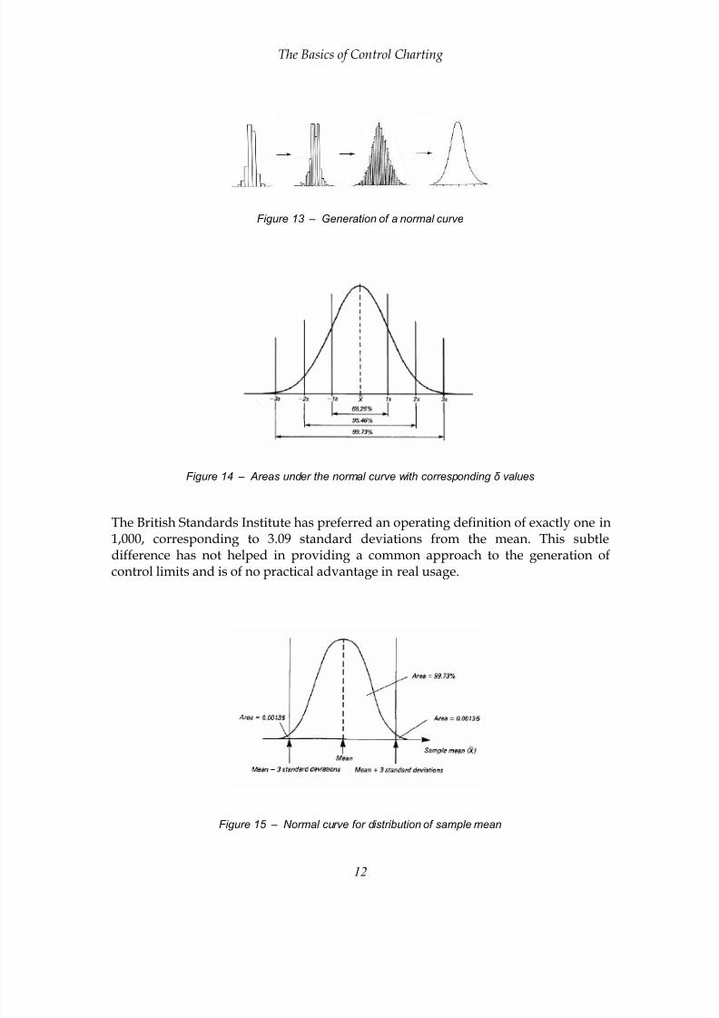
A brief summary of the normal curve is relevant here. Figure 13 illustrates how ahistogram approaches a normal distribution with the properties shown in Figure 14.In particular, for sample mean X, we have the properties shown in Figure 15. Hence,if we know the distribution is normal, it is suggested that control limits can then beset as shown in Figure 16. The chance, probability, of a point lying outside aparticular control limit is then 0.00135 (nearly one part in 1,000).




12

Figure 13 – Generation of a normal curve

Figure 14 – Areas under the normal curve with corresponding δ values

The British Standards Institute has preferred an operating definition of exactly one in

1,000, corresponding to 3.09 standard deviations from the mean. This subtledifference has not helped in providing a common approach to the generation ofcontrol limits and is of no practical advantage in real usage.

Figure 15 – Normal curve for distribution of sample mean




13

Figure 16 – Normal curve and control limits

8. SHEWHART OR OTHERWISE?

The Shewhart approach and the probability approach do address the question of theorigin of the control limits from differing viewpoints, and to that extent they are inconflict. Figure 17 illustrates the reasoning behind the thinking. In a great many casesthe underlying distribution is normal or sufficiently close to normal to be treated assuch.

It is then a logical step to argue that the area in the tail is 0.00135 when the limits areat three standard deviations from the mean. The drawback is that with no priorknowledge of the process we cannot assume a normal distribution. Hence the reasonfor placing the emphasis on the 3δ rather than the area in the tail.

Figure 17 – Probability and Shewhart charts

The Shewhart approach is the more correct in that it makes no assumptionsregarding the normal distribution, or any other distribution for that matter. It isbased on the principle 'if it works in practice, let's use it'. It is too easy to be pedanticregarding one method or another. We cannot ignore the fact that there are two bodies




14

of opinion. For those involved in the practical application of interpreting charts inoperational areas it should not be an issue. Familiarity with the actual calculating,plotting and interpreting is necessary, and the next few chapters will give you plentyof material to use.

9. POINTS TO NOTE

• It might be helpful, without causing too much confusion, to mention the workof a mathematician called Tchebyshev. He showed, that if a process is stable,89% of the time X will fall within the limits: X plus or minus three standarddeviations, irrespective of the form of the distribution. The same result holdsfor control charts in general, not just (X ,R), and provides a mathematical justification of Shewhart's approach (Figure 18).

• The Shewhart / Probability argument is less important than recognising thatthe limits are performance-based rather than specification-based. Performancelimits which represent the process must not be confused with limits based onartificial targets. The rule for detecting a point outside a control limit is justone of four commonly adopted rules for detecting special causes.

Figure 18 – Justification for limits set at + / - 3δ

8. KEY WORDS

With this general background we are able to set up control charts for both variable(measurable) and attributable (countable) data. The approach in both cases is verysimilar. Both types of charts require some simple calculations and, in the case ofattribute charts, reference to some standard tables.

The beauty of these charts is the effective way in which they convert staid,uninteresting information into a new form. The layout is not only easier on the eye,but also offers well informed insight for corrective action. Terms, symbols andformulae introduced in this Note are listed in Table 1 and the Appendix presents the




15

equations needed to calculate control limits for both chart types, sampled values (X ,R) charts and individual values (X,mR).

Key Word Meaning

Sample A representative group from the process.Run Chart A graph showing variation over time.

Stability Condition of a process whose natural variation willnot change if left to itself.

Predictable The result of process stability.

System The interaction of people, materials and machineswhich provides the environment within which we

work.

Common Cause A factor which is part of the system.

Statistical Control Operating within natural limits of variation.

Special Cause A factor which is outside the system. An unusualeffect.

Out of Statistical

Control

Not operating within natural limits of variation

because of the presence of a special cause.Grand Mean The mean of a series of X values. Also known as x

double bar, x

Central Line A line on the control chart corresponding to theaverage for the process.

Control Limits The upper and lower limits of the natural variationof the process.

Normal Distribution A symmetrical bell-shaped pattern. Readings frommany processes tend towards this shape.

Probability A numerical measure of risk.

Tchebyshev Name of a mathematician whose work providesstatistical evidence supporting Shewhart's practical

use of three standard deviation limits.

x Grand mean; i.e. ∑X /(number of samples)UCLx ; LCLx Upper ; lower control limits for X.

(X , R) Description of a control chart for dealing withsamples.

(X moving R) Description of a control chart for dealing withsingle readings.

Table 1 – Meaning of Key Words and Symbols




16

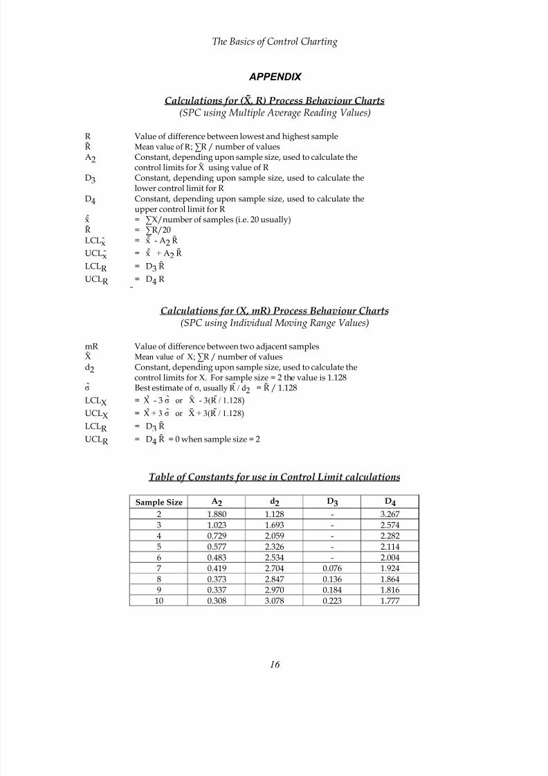
APPENDIX

Calculations for (X , R) Process Behaviour Charts(SPC using Multiple Average Reading Values)

R Value of difference between lowest and highest sampleR Mean value of R; ∑R / number of valuesA2 Constant, depending upon sample size, used to calculate the

control limits for X using value of RD3 Constant, depending upon sample size, used to calculate the

lower control limit for RD4 Constant, depending upon sample size, used to calculate the

upper control limit for Rx = ∑X/number of samples (i.e. 20 usually)R = ∑R/20LCLx = x - A2 R

UCLx = x + A2 R

LCLR

= D3

R

UCLR = D4 R

Calculations for (X, mR) Process Behaviour Charts(SPC using Individual Moving Range Values)

mR Value of difference between two adjacent samplesX Mean value of X; ∑R / number of valuesd2 Constant, depending upon sample size, used to calculate the

control limits for X. For sample size = 2 the value is 1.128σ Best estimate of σ, usually R / d2 = R / 1.128

LCL

X

= X - 3 σ or X - 3(R / 1.128)

UCLX = X + 3 σ or X + 3(R / 1.128)

LCLR = D3 R

UCLR = D4 R = 0 when sample size = 2

Table of Constants for use in Control Limit calculations

Sample Size A2 d2 D3 D4

2 1.880 1.128 - 3.267

3 1.023 1.693 - 2.574

4 0.729 2.059 - 2.282

5 0.577 2.326 - 2.1146 0.483 2.534 - 2.004

7 0.419 2.704 0.076 1.924

8 0.373 2.847 0.136 1.864

9 0.337 2.970 0.184 1.816

10 0.308 3.078 0.223 1.777




17

REFERENCES

Further Reading and Study

SPC and Continuous Improvement by Mal Owen, 1989

SPC and Business Improvement by Mal Owen, 1993

Understanding Variation by Donald J Wheeler, 1993

Statistical Process Control in the Office

by Mal Owen and John Morgan, 2000

_____________________________________________________________

This booklet is provided to users of The FlowMap System to provide general insights

into business problem solving and process aligned management. The key to bothof these activities is the discipline of 'thinking in systems and working on processes'.

This publication copyright (c) 2003 Management-NewStyle ISBN : 0-9543866-5-5 1st Edition, October 2003

Published by Management-NewStyle,Chislehurst, Kent, BR7 5NB, England www.firstmetre.co.uk

The FlowMap System (c) 1990-2003 David HowardFlowMap Software (c) 1994-2003 David Howard and Maurice Tomkinson

FLOWMAP is a registered trademark of Management-NewStyle

statistical proces control - david howard

Documents