vol., - dtic
TRANSCRIPT

11• • -•' W'r--" --".- . ... "; "_t_......____,- _--
--_.
FAA-EE.8046, Vol., Evaluation of AlternativeOffice of Environment Procedures for Atmosphericanh En2ergy Absorption Adjustments
During Noise Certification
k: Volume I: Analyses and Results
S0Alan H, MarshDyTec Engineering, Inc.2750 East Spring StreetLong Beach, CA 90806
October 1980
Final Report
This document is available to the U.S, publicthrough the National Technical InformationService, Springfield, Virginia 22161.
DTICC ECTE
6•. MAR 0 5 198Z
U.S. Department of lansportatlonf
Frdeml Avliaton• Adminishation

NOTICE
This document is disseuitnated under the sponcorship ofthe Department of Transportation in the interest ofinformation eaxchrnge. The United States Governmentassumes no liability for its contents or use theraof.
The method of American National Standard S1.26-1978for determining the atmospheric absorpticon of souwdhas not been approved by the Feleral Aviation Admin-istration for use in aircraft-noise type .!ertificaticnunuer Part 36 of the Federal Avlatinn Regulations.
W I M
il ::Ik•I
I' .:9i
•.I

Technicel R~eport DoCumentaltition Page,1. Repair No. 2. Go~v,nmirnt Azc~s~ia,, No.T Reiin' Catalog No.
FAA-Ll- 0j'U-46, Vol. . I.-.-.. - .. ~....-___ _______
A. Title and Subtile ~. -Oati
E'valuatlion of Al tcrnat lye Procedures for A~trmsp)NC; ______________
Absorptioni dJ ustments IDuritig Noise Ccr~ ificatloi A, .ne JraIsarion10 code
Volume [: AnialIyses aild Resultfs
~~~~.~n Ar r') -rgOrgan. zot~an Report No.
Alan It. Marsh Rt, rt 79260. Performing Orgavtisation Name and 4kildftsa -ý W_____________No. ______________
Dye ii:g itner itlg , I nc.275 Eas'*t Spr i ig~ St rue L I.Contract or Grant No.
,I~i), , ' B cci, CA 90806 _______________________
ki1U. Sponsoring Agency Nome and Address
DI.S.lepa r tmen t of ' Transpor tato Fiia Reor'edclral Aviationi Ainfiniscrotiunt
Office of* Ftnv ron)meint anid Lrnergy14SosrnAgcyCdWash01IngtlLoil, DC 20591 E!i
Ri cl"Iard N. led ric-k, Chli f of tilt., Noi se Pol 1icy and Regulations4 B~ranch of theNoise Abatement lDivilson of the( Off iue of Enivirctinment and Eniergy, was the
F'AA lTicliflerl (aIPro'j ect Manlager.16. Alistract111 ieWork repor ted lic-e va ,xtvinds that inl VAA-RI- 77-167, December 1977 to the problemof aI (- o tLkloil a i-c raft. noise / 3-nc tavce-batid spec tra menesuited at 0. 5-'s I nter-JVa I ,. Test - :ni s'euLi-a aire used to calcuenlate MI. , 1'NLT, EPINI., Al,, and SEI, Th vt0sL-diav s icte rumi a) the Limec of PIA'1N , anid at th e Lime of' ALM' are ad jus ted to acous-
I cl--et reie inud U ions, uising) theit, isheiu-bop rin ethod in Amen icanNa i oiiail SI aiiu:it-d k ,NS I SI . 26~-078 and appIlied, usinig measurements of air temperature
aId reII at IrP.'hum L l i varlmios hle igits ah:'-vc OWi grounid by ititegrat tog over thefruqueio'1v11 l~a, i Ie'pisshoand (if idt.-il lieters and by calculating the absorption
It. tilt u 'arIt Iillid-center 1'rLeq tlie! n-111 n V. SAF. AR11866A is al so used with the ver t i-I -piti c tmjrl-l~uc/hmii tklatal an1d -di th dat~a at 10 il to determine adjustments
It-rein Lus t- to- re ferenc-e eond it Iohs . Th~e adi ustinInhd r ple O nisedat.mvi mehd ar riihie too :1rua
Vol ne isc riles thec anial vss ail( ic-;eul Is of the study. Volume It presents theC~flil'ULi.t J'pli-rgt am tl:J was.L developeLd anid il lustrates its usu. with a test case.
oI a-I I I p re Seit, il;s hI ,s of at r enna -t Inn dule to a tmos phier ic absorp tion ove r a 300-nilpa;it Iti. At t eriiaaLIo!ls wert- Ca'llu I aced usling, ANSI SI1.26-1978 for pure tonies at band-
ceot ~r re(iie(- u. ad for Un-reu no~lse spect ral slopes b\: a hanid- integra tinn ti~ethod,;iodc us I ig SA\E AlI566A . lireniul of thle five miethuds , the tab les cover' 34 air tern-lie rat tir-e, 1" rum 2 to '356 C, it)0 reIalatIv VC humi dirt ics f rom 10 to 100 percent , and 24mm Iniflo I hanld-Center U reItwlcit-ni(u from 50 to 10,000 liz.
17. Key Words 18. Distr,bution StatemenitAtMospIheric a-iso rpI oiol r,f Solilri Availlbi~l itv unlimi ted. Report Is avail-iirvraft nioise cer-t I f tecat L iii able to 0he public through the NitionalA'451 q 5.26- 19 78 'Feleuhn al IniformaL ion Service,
S~t: ~l-P8(0ASpr inp fifvld , VA 22161
19. Security Closst]. (of this repart) 20 Security Clessil. (of this pageg) _[ I. No. of Pages 22. Price
11"I. Iil,;S IF IL-1 Ut c l ss f ed215
FarmDOTF 100. (872)Reproduction of completed page -%iihorlaod
Sectiton Pag~e
Description of Test. s.. ......... .. ..................... 9. 7
Test-Time Mttoro log icall I)t, ta..... . .. ................... ... 101
Sound Propagattion Pails . . . . . . . . . . . . . . . . . . . . . . 12
Data Analysis and Adjustment Proceduresr .............. 121
Description of Band-Integration Procedure ............. 126
Results of Comparative Evaluations of AlternativeAtmospheric-Absorption Adjustment Procedures ........... 140
Measured Perceived Noise Levels and A-WeightedSound Levels ................ ......................... ... 141
1/3-Octave-Band Sound Pressure Levels at the
"Time of PNLTM ................. ........................ .. 151
Atmospheric Sound Absorption Coefficients .... .......... .. 155
Band-Level Test-to-Reference-Day AdjustmentFactors ....................... ........................... 159
Effect of Different Adjustment Procedures onReference-Day Sound Pressure levels.. . ......... ............. 184
Effect of l)ifferent Adjustment P'rocedu~res on
Reference-Day EPNL ad SEA ....... ................... .... 188
5. CONCLUSTONS .................. ............................ ... 199
6. IU.F',"RENCES ........................... ............................ 203
Acoession For
NTIS GRA&IDTIC TABUnannounced []Just if ent ion-_
S~~~By .........
Av ,ili ;I l L-y Codes
,ind/ur
fCl,I .. .... .. . . ..
Ii
J) -j~

CONTIENTS
I NTRO1)tUJ r 10N . . . . . . . . . . . . . . . . . . . . . . . ... . I
I TFCT LZ9 TOPEI CONVI: I'tNS ON CALC:ULA-IONSOF ABSORPTION-ADJUSTMENT FACTORS FOR BROAI)!'AND SOUNDI) ... . 9
Spectra at the Source .. .......... 1
Spectra at the Receiver . . . . . . . . . . . . . . . . . . . . . . 17
E'xact Test.-to-Ref erence--Day Band-Level
Adjustment Facos..c t or ..... ..... 25
Approximation of Source Band Levc-ls byliand-Integration Method. ............................................ 27
Approximation of Source Band Levels byBand-Center-Frecluetncy Method .. ...................................... 37
Approxtimate Test- to-Ri ferecne.-IDaBaud-LEvel Ad )I utiTIVO( Fact )rs..... ................ ............... 40
3. EFECTS 0OF NON- IDEAL, F ILTER CHARACTERI1STI CS ONCALCUiLATIONS OF- ABSORPTI ON-ADJIISTMENT FACTORS .. ................... 45
Ft It er Tra1nsmission Response .. ...................................... 45
SpectIra at the Sourc . .. ............................................. 2
Spectra ait t~he Receifvr... ......................................... 54
Ad Itistmient F;actocrs...........................61
4. ADIJUSLME'NT ~FAtIRCRAFT NO ISE D)ATA FROM TESTTO REFFEREANCE METEORO1LOC I tAT. COND ITIONS. .. .......................... 75
Req i rertients for Atmospher ic-Ahsorpt ionAdjlustments IDur fng Noise Certification. .. ................... . . . 75
ReqJUirement~s [or a Layered-Atmosphere Analyst s... .. ................ 78
Re F runce Meteo rolIog 1 '1il Cond itin ......... ......... ........................ 81
.4iwiival Requl r''mnikts ()f VAR 30 for Al reraftN I .w Measioremen t and Aiia I vsl I.. .................................... 82
Basic Ass~-umipt ions Related to AtmosphericAhb;crpt Ion Ad justments .. ............................................ 88
Ass'imp t fiOns Regardting Calcuilat ion ofTone--L:(rreC t.Ion Fac tors. ............................................. 9
As'; imp~ iti s Regard ing Cal cul atiton ofIhirat ion-Correct ion Factors .. ......................................
ILLUSTRATIONS
Figure Page
I. Power spectra, GS(f), of the sound pressure at the source
for several spe(' trl r lolIpes ................................. 15
2. 1/3-octave-band sound pressure levels, LS, at the source
for sound pressure spect, raIl donsities of Fig. I and Ideal
filters . . . . . . . . . . . . . . . . . . . . . . . . . . . . 10
1. 1/3-octave-bano sound pressure lewvL, IR, at tie receiverfor sound pressure spectral densities of Fig. 1. Ideal filt'-r!ý`
Ali* temperature of 25° C; r, iweh lidity (f 70'7; air pressure
ofI .0 standord aitmosphet, re. Propagaation di stances as noted.Attnlluation by aL.mosphchri(c absorption onlVy no spreading loss. . 22
4. L/3-oct tave-band ,dsound pires•,ure leveIs, IR, at OIL recceiverfor the samti condition as for Fig. 3, except a relativehumidity of 107 instead (e! 70,". ..... ................. ... 23
5. Attenuation (diffference (hlie to atmospheric ahsorption between
hand levels at the source, LS, and band levels at the receiver,
1,R) as a function of frequency and propagation distance. Two
relative humidities and band-level source spectrum slopes.
i r temperature is 25' C" air pressure is 1.0 standard atmosphere.',1,;i v iter s. No gonlietri c spreading, lossn.. . ............ 24
0. [-'uior exatt band-level ad j ustment factor as i function of
f'requency and propaglation distance.1 Difference in hand levelat the receiver under sim.lated reference and test atmosphericc'nd [t ions [(IR at 7W% relIatiwy humidity) - (1,R rit 10% relativehumidity) ]. Air tvmlperature is 25* C; air pres'cure Is 1.0standard aItmlosphere. Ideaol f1 1 te rs... . ...... ............... 26
i/. Hlypothetical spectrum of a ircralt nois(... ....... ............ 29
H. Ccunp;Irisom of hand-s lope i•st imict ing prrocedlures for certain bandsfrom hypothetia;l ,i rcroft noise spectrmn of FI.,. 7 .. ..... . ".
o. llu:;t at ions of str;a igh t-linn, approximat Ions to suund pressurespectral density G;M(f) with slopes 9. and 91 over passband ofideal filter wI hIi hand center frequency f, ...... ........... 33
10. l.xample of deetermInat Iw of (1 ) attenuation, (2) accuracy of;ipproximlatVe hand-tntoegratIon method of calculating atmospheric;ibsorptlon, rind (1) exact band-loss adjustment factor from test(10% relative humidity) to reference (70% relative humidity)meteorolog ical (I (it ions. Air temperature is 250 C; airpressure Is 1.0 standard atmosphere; L•pectral slope at the sourceis -12 dB/band; Ideal filters; sound propagat ion path length Is600 m; no geometric spreading loss ....... ............... ... 35
ii
9j

Figure Page
I1. Illustration of ability to accurately calculate atmosphericabsorpt ion over a sotund propagation path using hand soundpressure levels it the receiver. Calculated band levels atthe source are compared with known, exact band levels at thesource for three sound propagation pathlengths, two slopesfor the pressure spectrum of the sound at the source, andtwo relative humidities. Air temperature is 25* C; air pres-sure is 1.0 standard atmosphere. Sound spectrum at thereceiver is approximaited by band-level slopes over the lowerand tipper halves of the passband of ideal 1/3-octave-bandfilters. Absorption over the propagation path is calculatedby integration over filter passband ...... ............... .. 36
12. Similar comparisons of ability to accurately calculate atmo-spheric absorption over a sound propagation path as in Fig. 11,except that absorption factor for band sound pressure level isdetermined only at the center frequency of the Ideal filtersinstead of by Integration over the frequency range of the pass-band. Air temperature Is 250 C; air pressure is 1.0 standardatmosphere ................... .......................... ... 39
13. Example of determination of exact and app)roximate band-lossadjustment factors for differences in atmospheric absorptionunder test (10% relative humidity) and reference (70% relativehumidity) conditions. Air temperature is 250 C; air pressureis 1.0 standard atmosphere; spectral slope at the source is-12 dB/band; Ideal filters; sound propagation pathlength is600 m; ti0 geometric spreading loss ........... ............. .. 42
14. (Cofilli. oonof o ipproximoaiLt and exact band-lo;.,; adjustmentfactors for idevi filters. Difference in source levels(,S 1 0 , 10 - LS 7 0 , 10) calculated from receiver levels, lKIO.determined for 10% relative hltmidity (test-day conditions).is:;tiing first 10 and then 707 relatlve humidity (reference-day conditions), compared with difference In receiver levels(lR, 0 - l.RI 0 ) for 70 and 10% relative humidity. Air tempera-ture is 250 C; ii r pressure 1. 1 .0 standard atmosphere. Threesound propagation pathlengths; two true slopes for the soundspectrum at tho source; and two approximate methods for cal-culating atmospheric absorption: integration over filterpassband and absorption at band center frequency, f , only . • 43
c
15. Pow(er t rainsmlssion rsponse (4 I /3-otaV,-hII;nd fII ters 4...... 8
16. Tran sni ,s Ion-loss r vsI itis(. c I inractv rIst Ics o f /3-(cLIvtband filters In real time a;mialyzers c-ompared with responsecalculated from "pract icali- filter" transmiss ion-responseequationn; f is band centr frequency ...... .............. 51
C
iv
L•. .-

Figure Page
17. Power spectra of the soound presstire at the soturct forcaleuilat Ions of band levels at thet receivwr with 'pratctival,
rather than ideal filters . . . . . . . . . . . . . . . . . . 53
18. Etfect of filter characteri st Ics on hand level at the re-cei yver for various slopes of the sotind pressure levelspectruim at the source. 300-11t sot id propagna tion ittLhlength;707 relatLve humiditv; 25' C air tc'Mleratu re; 1.0 (-4tandard
aL mospliere a;ir pre tr ..................... . . ... . .................. 58
19. Same ;15 Fig. 18, except ItOZ reltativ, humI(dIty .... .......... ... 60
20. Effect of filter transmlssion response characteristics onband level at the receiver for three sound prop.igationpathlengths, two relative humidities, and a slope of the"SMound p)reSSUI-e leve' spectrum at the source of +1 dB/band.250 C air temperature; 1.0 standard atmosphere air pressure. 64
21. Same is Fig. 20. except sloape of sound pressure level.spectrum ;It the soirc'e is -12 dii/band . . . . . . . . . . . . . . 65
22. l)ctermination of hand-loss adjustment factors when bandevels at the receiver locat ion are calculated with the
filter transm Iss Iton-response characteristics of the practicalfilters from Fig. 15; compare with results for ideal filtersin Fig. 13 ................ ........................... ... 69
23. Comparison of band-loss adjustment factors, calculated atband center frequency, f,., only and calculated by integrationover passband of Ideal filter, for receiver band levels deter-mlined with prart hal-fI ltr transmissIon-response characteristics.Compare with Fig. 14 for recciver levels determined with idealfilters. See Fig. 22 for definition of terms. 250 C air temperature;1 .O standard atmosphere air pressure. Three sMtond propagationpathliengths, two sound pressure spectrum slopes at the source. 72
A. Measured verti cal profiles of air temperature and rctativehumidity for test cases; also i)rofl.ts of difference hetwenat tmospheric absorption coefficient by SAE ARI'866A at '3150 tlzat height anod at 1(1 m I)li ilht ........ .................. ... 104
r.. Measured vertlcai profiles of molar concentration of water
"vapor for test c(ses; reference molar concentration of watervapor at 25' C, 10-percent relative humidity, and one standardatntmosphere of air presstire is 2.18774 percent ............. ... 110
26. Geometrical relatlonshi ps heLwetn aircrnaft aInd microphone atdifferent re, lative tlines; durin, a flyover.. ................ ... 115
V

SIpu r'u Page
`7. Ie linIt lIon of quant It le, used 'n calculating angles g , e r, and J;sound propagation distance PD; and aircraft height above themicrophone height at the '.line of sound emission AHS ......... ... 117
28. Illustration of procedurc for calculating incremental distances,along sound propagation path of length PD from R to E, whichcorrespond to heights IIM(K) where meteorological data weremeasured ..................... .......................... ... 119
29. Illustration of rules for calculating band-level differences . . 134
30. Substitute slopes for 1/3-octave-band levels of broadbandaircraft noise in the free field ............................. 136
31. Variation of normalized PNLT and AL with time during aDC-9-14 flyover, from run 272 ................................ 142
32. Variat ton of normalized PNLT and At. with time for theRalsbeck-Learjet, run 12 ........... .................... ... 150
33. Aircraft sound pressure level spectra at the time of occurrenceof the maximum test-time tone-corrected perceived noise level,IN LNtest . . . . . '. .... . .. .. ... .. . . . . . . . ".. . 152
34. Pure-tone tmospheri' sound absorption coe ficients by
ANNSI S1.26-1978 and SAE ARP866A .......................... .. 156
35. Band sound-pressure-level ad.lustment factors at the time ofl'NL,'l'Mtc st for 1)C-9-14 rims at nearly-equal sound propagationdistances, 111), and emission angles, ', but different meteor-ol( 'jia1 ('ondititons flIong the sound path ..... ............ ... 160
30. Ililustration, for 1)C-9-1/4 runs 272 and 358, of differencebetween reference-day sound pressure levels calculated byadlustment procedtires (2) and (3). Propagation distances andsound em ission angles are for the time of PNLTM1t........168
37. Band sound pressure level adjustment factors at the time ofPNL'rltest and of ALMtest for DC-9-14 run 374, PD = 369.4 m,1 = 113. 1. . .................................. ............... 170
S " 38. Sound pressure level spectra for test and reference meteor-ologit'al conditions from D)C-Q-14 runs 358 and 374 at nearlyequal sound-emnissi on a;ng1les utit dif ferent propaga tiond 1st :itcs ..................... ............................ .. 173
39. For nominal ly equal sound-em ission angles (110.50 and 113.10),Illustration of effect of choice of atmospheric-absorpt ionumodel on ability to extrapolate reference-day SPLs .. ....... ... 177
v1

Figure Page
40. Band sound-pressure.-level adjustment factors. at the time ofPNITAtest and of ALM test for Raisbeck-Learjet , run 1.2,
P1) = 1925.7 m, 4 = 135.2.. . . . . . . . . . . . . . . . . . . . 181
41. Sound-pressure-level spectra for test and reference meteor-
ol og• cal conditions for RIaisbeck-Leen rjet at time of PNIM testor ALM tet, run 12, I'D= 1925.7 mn, ý= 135.20.. .. .. ............. 185
42. let-tO-Lo-reference-day al.justment fat t. ors by thv four adcjustment
l)rocedures for PNI,T and Al, for IC-9 test cases (runs 272 to 378)
Snud Lear.j et (run .12) ............ ... ...................... 196
v,
ivi
iIi
-.

N imibe r V: 1)e
I Description of aircraft used for test cases ........... 98
2. Test and airplane parameters .... .. ... .. .. ... .. 100
3. Meteorological conditions for test cases 3.03
4. Engine/air'lane parameters for I)C-9 rnms .... ............ ... 145
5. Measured and approximate durration factors for FI"'NI and SE, , 148
6. Comparkion of results, from present study with those
I: 'rou R01'. 25 I'or fw, IDC-) r .. ............................. 189
7. Conmprison of test-t ime quannt it ies calctilated by BBNand by present study (P. S.) for data obtained from BRN .... 192
8. Summary of 1'reqctency-weI,,ht ed and tLime-integrated noiselevels for DC-9 and Learjet test cases where meteorologicaldata aloft were meastired .......... .................... .. 194
9. Summary of f recptency-weighted and time-integrated noise
LewIvts for 727, IIS-748, and Beech Dlebonair test caseswhere only surface meteorological data were measured ....... 195
viil
IL-
*a u
9~ a 7 N S43 t Mh'
a (N
k 41A bd
CL a.

.1 .
ACKNOWLEDGMENT
It Is a pleasure to acknowledge the niony helpful suggestions and con-structivL' comments provided by the author's colleague Dr. Robert i,. Chapkis.
f ' i
-. . -

EVALUATION OF ALTERNATIVE PROCEDURES FOR~ATMOSPHERIC ABSORPTION AD~JUSTMENJTS
D)URING NOISE CERTIFICATION
VOLI.MI I: ANALYSES AND REM)I[ iS
1. INTRODUCTION
TO certify the noise of aii aircraft, the only approved procedure for
adjusting measured sound pressure levels for differences between atmospheric
absorption under test and acoustical-reference conditions uses t.he method in .the Society of Automotive E'ngineers (SAIE) Aerospace Recommende.d Practice ARP866A
'V ror calculating atmospheric sound absorption coefficients. Th1at atmospheric-
absorption model was developed by the SAE1 A-21. Committee in 1962 and 1963 and
pub I shied in 1964. It wasi, re,- i Ssiid in 1975 ;is ARIP866A' and is tiso~l to adjlust1I t*omi test- -o- refereonce coniI tionis in Pairt 36 of the l'edura I Aviation Regulations
IAR3'1) and In Anne1LX I6 to the Inaiernat jonal Standards an1d Re'Commcndc~d I'ract lets
01 II Iie lt rila i Iona .1 C iv il Aviation Organ iza tion. ARP866A Is alIso incorpornted
in Internat~ional Sta-ndard IS 3891 as part of the procedure recommended by the
International Standards, Organiz~at ion for describing noise around an airport.
The American National Standard Method for the Calculation of the Absurption2of Sound by the Atmosphere, ANSI SI..26-1978 , was published in 1.978. It contains
a ser-ies Of euaIWitios that permit calculation of the atmospheric sound absorption
Coefficient for a pure-tone sound with a frequency between 40 and 1,000,000 Hz
(at an air pressure of on-2 standard atmosphere) . The equations are stated to
be apyplicable for air temperat'tuires between 10' and 4 0 ' C, relative humidities
between 10 and 100 percent,. and air pressures less than 2 atmospheres. The
analytical vxpre:is ions that formn the basis for thie calculation method were
\'alidatcd by laboratory tests 3over a wide range of atmospheric conditions
and frequtencies, spe'Cificallly frequencies from 4000 to 100,000 Hz at 1/12-
octave. intervaks, temiperat'ires from -1.7.80 C to +37.80 C at 5.6' C intervals,
adreL'at~ive Iii ndi ties fromi 0 to 100 percent at 10-percentage-point intervals.
The analytical model!i- ARI'866A for atmospheric nbsorption is based on air-
craift flyover nois- (data aýnd ;in earlier and less-compi tet thieoret ical understand-

I ig 0l f h LIICVarious phys i (', I tiechanII I snis t hao t [LIe anllvi I ica I mod n it)1 in ANS I S I .'6.
I n A RP866A the atna I y t ica I mode I i.s a )ppIlied to b)roadbI and sot nd spec I ra a I)a I I ~e
by I./ 3-or I / I-lW tavc-lbaii(I f I Ite(rs w i UIlt In L regard for spec t ra I ,Ihapeo tt , * "opg' I-
Li on d istance. Acit tnai iion over a pa 11 length is calculated byv dete~rmining ;tit
-II)so rlt ion (oef J*1 c ent (at a part: I ctilIar frrcqlteny) and muILtIpIl y log I) y 0he (11is-
Lance .The nominal band center frellueticy is used for cal cu htaionS at ce-Lnter
frequenCHCIes c,, 4000 liz. To allow for thle rapid high-rirequency spectral rolloff .rate often encountered In measurements of aircraft noise, alsorptir'n coefficients
for 1/3-oct-ave band,, with center frequencies front 5000 to 10,000 l;, are calculatc~d
using the nominal lower bandedge frequency for those bands.
Sec tion 5 of ANSI S1.26-1978 provides generail guidance, oil how to apply the
pure-Lone ca lculatio 1(1metLo~d of the Sta-ndard LU) the problIem of cal cikiatit I n th
:ib.-;or'L ion loss experie~nced by a sotnid wi i tiu.enrgy dilstributed over a wide 1'r.--
q uenicy range and analyzed by f a ioaIn aeIadil t ers. I t recommends
ovalI ua t ion -of a paie of i ntigra Is over a range of frequency for vach hand. The
pressure spectral density of the sound must be known. Additional guidance Is
given in Appendix I-' of thle Standard regarding a method for numerically evaluating
the i ntegra Is (if Section 5 when it is ne0cessary to consider the power transmi s-
s ion resp~onse of prac i cal. t/3-octave-band [il ters and when OC' pressure spectral
dens fry of the Sound atl thu begI il ino, of the propagation path canl be approximated
by a func t on p ropor t iona 1O to freqjuentcy to sorte power.
A stUdy 4 was conducted for tho FAA in .1977 to develop a digital computer
p)rograml, in the extended FO)RTRAN I.V programming language, that was capable of
Calculating ad~jU'-tment factors to be applied to l/ 3-oc tave- band sound pressure
levels to account fur di fferences iii atmospheric absorpt ion losses experienced
under test and reference meteoro log I al conditions over anl assumed sound propaga-
toinn pathi. Thel( priogran compotied pn r.- tone atmnospheri c absorpt ion l osses by tile
miethlod IIn the t hun- proposed, but es sent I I I finIna1, version of ANSIT S1. 26-1 978.
TIheI in e),ra Is were nurser i call Iv v;iti a ted by tile approx imationO scheme out iineId InAppendix LC of Ltle Stanldard aiid, 111 1i10or0 detailI, in) 4-f . 3. 'I'llu pressure spec tral
denls i t of tiILe SOUnd IrtL ti( henilc roplic~ne was es tima ted by a s implIe power t u'ic tion
over the theoretical bandwidth oif 1/3-octave-hand filters. The slope 9. of thle line

T -11(or t he exponent of the ',ormlr I I xed I requency , no rmi1 I. led hy t he evxa* t baild
gennmetr Ic mean f -quency , f ) was obta ined from the I i d fe relnce hk-, weeci t hIeC
level in the band below and the level in the band above the band Wf Interest,
Thus, at a general frequency f., the pressure spectral density was propor-
tional to (f If )j
The numerical integration procedure developed for the computer program
In the 1977 study used the proredure described in Refs. 2 and 3 for approxi-
mting the frequency dependence of atmospheric absorption by a power function
(F+I/f )K over small ranges of logarithmically spaced frequency from f to
f .1 - With those applrox mat .ons for the absorption function and the sound
pressure spectral dens ity, thie general Iintegral express ion co)ld be replnced
by a summation of intLegrals .acih (if' whi(cih could be integrated exact ly in
closed form.
The power transmission response of the 1/3-octave-band filters was
assumed in Ref. 4 to be that of Ideal filters because the objective of the
analysis and tile computer program was to start with 1/3-octave-band sound
pressure level.s measured at some rec'eiver location and to calculate an
adjustment factor to he added to the measured band levels in order to deter-
mine what the band levels would have been had the sound propagated through
an atmosphere with acoustical-reference meteorological conditions rather
than tile actual nveteorological conditions existing on the day when the band
lvels were measured. The assuim,,--ln that the filter response was that of
an Ideal filter was considered to be most appropriate for that problem.
T['he assumption of ideal fil.ter-transmilssion characteristi(s was justi-
I led on 1h1' grounds that (I) the pressure snectral density has to be estimated
from measured band levels, (2) there is no uinique, one-to-one relationship
hetween a set of measured bnnd levels and the true pressure spectral density"i- tile sound that impInges on the microphone, and (3) there is no way of
knowing how much, if any, -he indicated band-level value is influenced by
energy transmitted in the stopband frequency ranges due to inadequate
filter-rejection capabilltv.
3

The assumption of ideal filters was also considered to he consistent
with the other assumpt ions regardinog the, approximation of tile absorption
fcnw Lioln, thV 'IdWIMC~y Of tho number of hor izontal l 1ayers inito wihichi till
it i'loispher(' hod Ititi stibl (I vided aind Oiver wlic lei ti-st-day miteLorcilogit-al
coticif I IIiii ccuildc be iissiiieiticivd ( ho iclilot ;lit , .i1d the 141)11 etig th( 01 Ii stttild poIiiia-
,.; ut pat l itil . 'lii sounidc p~rO11.piga hill pa](11 wot";i tit d to he ;I si ughc si roi Ilg t I I fti,
Cr~ al L(It 1vai I cuti sotirccc' I oc"it I. ion t (I Ii I t(i I crophtone', lop~, I cc t 11-1) ;!Iccv beicci I 1ip,
(rfatfn ftl ieto fpoaaina resuilto (t'empecature-
thatthevarious cornp lx no ise souirces, coultd be repl[aced by a single
G iven those -Issump t i ois, the act mosphierice absorptioun model of ANSI S1 .26-1978
was5 appliIed , loitsng thIe spec ifi iltmne r icol In l %.,,:.: tion ie thod desc r ibed above,
- ~~~to ri I nl kito 'il b;til actistittetit act or.s Ifor dif herenoces bctwouei atmiospher ic
alb,,olcpt it'l 1 itscs 111110r tec',t-doiv tind rutIr cfrer'c meteciroliogi cal
rond I t I Ons . 1ice ti1100 hd was a pl) it'd to , 1/ i-oc'tave-band solund pressure
I eVeh Fr iom q Itminl.a Led level-f.1i git a irecraft flIyover nolIse inca stirement s Hac
set of 24 level-,. was ;cssumtttcl tO b10 complelte with lit band levels, missing
b(caulse oif' contaminatLion by Iit igh-level background no i.-e . Two test cases
wi tih cli [ reot spectralI shapes, propagation path lengths, and test-day me teor-
ological. conditions were uxatiineci as a means of checking out the computer
p rogratm and ill us trating Lice tiagnic i de of the band-adjus tmen t factors.
T*R I1CIL [lecOpof tueV Ic77 stt(dy Iin Re'f .4 was l imited, as indicated above,
VSt-cu.e Lio I I y to the dIOVe Optlient oft ai compuiter program to uise thle atmospheric
abso rp t Ii on itodo I ohI ANS I S 1 .20- I ) 8 aind to I ilp I enien t the general recomnmenda tions
til tlie,, stanuid rd 1cegarMdi up, It oc' ;c I (-i I it I ott OF atmosplcc'rlc absorption loss for
a stud 011 no i S. ost l [itIttitdojec:Livc', It was not necessary to
Inc I ud tueL rC;lsib iIit y Of V\;lmtuint 0og / 3-octave-hand sound pressure levels at
0.5-s intervalIs tic otighiio ;iia f 1vove r or to cal (culate any psychoacous t Ical
litasize ,or tLL clVe lop at mtil'liod(i f es timatinog prc'ssuire spec'tral densityI
functions whcen a complete set oIt 24 hand levels (for center frequencies
from 50 to 10,000 Iiz) wais not tivailable because of c'ontaminat ion by background
4

noise, or to eva I uate ditf ferenc(es bet ween the method and all torn it iM e Ie',t I5.(of calculating ahsorpt ion- loss ad jIustment factors. Ifowever, the progr;am
that was developed did consider the problem of calculating abso'-;ionlosses over segments of the sound propagation path through horizontallayers of the atmosphere defined by the heights where meteorologi al
data were measured.
Paragraph (d)(2) of Section A36.9 of Appendix A of FAR 365 requiresuse of a "iayered-atmosphere" procedure for calculating atmospheric-absorp-
tion adjustment factors when the atmospheric-absorption coefficient at
'3150 Hz over the sound propagation path from the aircraft to the microphonevaries by more than ! 0.23 dB/10() m from the value r'alculated using theair temperature and relat ive humlidity measured near the microphone at aheight of 10 m above the ground stirfaice at tOe time of the ilmeasurement
I'lre layered-atmosplhere prOC'edU re r-l,|ires that the - atmosplhere he cIivld, dlinto horizontal stratii no thicker than 30.5 ill (100 ft) The average nirtemperaturt, and relative humidity n must be computed lor each layer from
Iteasiurements made as a function of height above the ground surface within25 minutes of the noise measurement and interpolated to the time of the,'as't.a reomen t . rthe avcerage temperatures and relative humidities must be
used to calculate average absorption coefficients for each layer. An averagea,'ttenuation rate over the total propagation path must be calculated from the
rotio ol the s.im of the attenuations over the segments of the pathto the total propagation pathl ength. That average attenuation rate (insteadof the Liate calculated simply from the air temperature and relative
hunmidity mre..stured at the 10 m he ight) must then he u.sed in making theabrsorlpt 1( :)(1.ji.strments in ai'•'-rdance with Paragraph (d) of Sec'tion A36.11of Appndix A. All albsorptinn coefficients are to he calcul ated using
SAI,' ARI'866A-1975.
Thl pturpolse vof tihe stidY descrilbed in this report was to employ. .ti.i, rreas.nired a i t' r.l ft nol' i;se and actcompanying meteorological data in a
c'omppIrlt iw, y vll u; Iion el di ffer,,nt procedres for determining test-day-to-re ferevn,-d;y aitmospheric-absrr tion-loss adjustment factors. The studyrequired rr lith-,r duvevicrpnrct a'id extcnsion of the digital computer program
reported in Ref'. 4. Tlic rovised program can perfform all the additionaltasks noted above as being outside the scope of the Ref. 4 program.
5
A.
Four a I ternic lev procedur,'' 1 fur ea ,1 I.ItnI ng I I'- c ot Ive-bal at il l II It'. rI,-
obsorpt ion ld.just men t I ictoý s were in I tIlded In thI I st ud\'1 'IIvv Wort,,
,' mb'wtrpt ioh oe;ft i 'it' .0t and hand attenuation by SA[ ARP86hA-I1W'
-ndait .m LetiritLogItcal dat.aL meistured olity at 10 Ill
* absorpt Ion cOefI I il ents and band attenuatit 9 by SAE AR]'866A-1975
a I ayered-atInosphere 0 a, I sy I ss t ing lilet-tvirologl c.i dat-I measured
at various heights
* aihnorption coefficients by ANS I S1.26-1978, a band-Int•grat ion method
to calculate attenuation, and a Ilayered-aItmosphere analysis using
meteorological data aloft
* absorption coefficients by ANSI SI.26-1978, attenuation calculated at
the band center frequetnicties only, and a layered-atmosphere analysis
using lneteoroltogi(,a1 daita alI(oft.
'flit, report is; organized Into) three Voliumes. V, unime I describes the
nonlywes that were perftormed olnd presents the restilts. Volume II contains
the listing (i' the statements for the computer program, the input data for
a saNflpie test case, and the cor responding moutput listings. Volume Ill
sUt)pl ements the Information In Volumes I and II with extensive tables of the
at tentiat.on cautsed by atnLosplihertc ihsorptIon over a 300-mi path. Attenuation
VAIICl ,r1' coiriplIltd for iVt' meWthiods for each of 140 combinations of 34 air
temperi|' tires: ind 10 c re:ntivye humidities. The tables permit a variety of
('i)mpi•ra|riv,. iiiila vses tI tilie differenwes betwee n the analytical atmospheric-
;lbso~rpt. ionil mode l.t o1" ANSI S l .20-1978 anld SAI" ,ARII866A-1975 and between the at tenuil-
I i(n :It Owc h;and center frequtency fVor a plre- tone sound and the at tenii;ition
['(t- br(:ldhaind .qm, ds with renot at .;lopes of +1, -6, and -12 dB/band.
'1vThe aInal voes and restilts I'resented here in Volt ue I are contained in
•. Sect i~ms 2-6. tlonsq 2 and u dlescritr the' results of ,ln analytical study of
H ft,ll1,t'; t 11o dlfferenl. aitmo!4ph ricr t c-ncdittrns and I/1-oct.ive-b;and Filter-
I li lsoit tlo -rtesp(onse charactr rit; i(':; on t the talculat tion f atlmosplhriv-
;ihso rpw ion aid ustment Ilacto Vrfor broridl•i;nd s;ound, The manwgnitude of the errors
tha•t cao wt ciilr ill tlhe VI1tlyo; t itthe balnd Iewv i s ;it a dista|nt receiver, and the
values et lifl, band Ilvels when adiuisted froqm test to reference condit ions,
irC C.lt'Icllit'ed I-or prayct ical filters meeting the minimum transmiss ion- loss

requirements of ANSI S1.11-1966 for Class II filters!' The accuracy of
determining atmospheric-absorpt ion adjustment factors is demonstrated for
hand- integrat ion and band-center- frequency methods.
Section 4 describes the basis for the new computer program for calcu-
lating atmosJpheric-absorption hand-adlustment factor.,. The program was
used to evaluate the differenct-: among the four procedures described above
for cal cirl.it ing band-adItistnint cu fctors. ,va I tint Ions ore presented in
terms ofl pIerceived nol:se t vo,,l, [c t,-torrected per0iC'i Vd n0ise level,
ef-ectIVe perceived noise level. A-weighted sound level, and Sound exposure
level for each of the fo ,- proc(edures for nine sets of a'tual aircraft
I Ifyo yver noise ineasureoments fronl jr't- and propeller-powered aircr aft.
Concl.usions conicerning the alternative procedures for ,etermlning
atmospheric absorption losses during an aircraft noise-certi ficat ion test
are drawn from the analyses in Sections 2 to 4 and presented in Section 5.
7
-- a-
€-j

2. EFFECTS OF ATMOSPHERIC CONDITIONS ON CALCULATIONS OFABSORPTION-ADJUSTMENT FACTORS FOR BROADBAND SOUND
k ii'torS, lotr :IhliII(r ta)(r~in Io~oes was, pet-I irmid inl1W jwil The f
I" rSt phase C oil 8 stv d ofI mal ysv-5 to s I lw t he va I i d I t y, (r neved I ii r ref I ine-
ment , of tile hand-adjustmtemt mlethod of Ref. 4. The second phase Included
development of a n.'w computer program aud evaluation of four alternative
procedures for ad~ju-t ing various aircraft noise signals from test to
neerne atmospheric conditions. ThsScindsussthe analyses
t hat werv conduc'ted for the f i rs t part of the first ph;z..3e for which the
fit~ers wero assuimed to have ideal t transmi ss ion- response characteris tics.I
The most-c rit ical !ssuv in developinug any method for determining
hanid-odtdistmntvi a'*ctors to ;icenunt for ltopeicasrtinIosses is[ licw ttO obt ain a good vstimate, Of the true pressuire 1.ptctral1 dens ity of thlesound that Impinged onl the microphone. For this reason, the original plan 4
for assessbing the validity of the method of Ref. 4 to account for atmospheric-
absorption losses was to obtain a narrow-band analysis of sampler, of aircraift-Inoise measurements for wh [cli I / -octave-band sound pressure levels and test-
day meteorological data were also avail lable.
Na rrow-band AnllYsesH were oht ained at thrveQ different times (before,
ilvar, ind( il*Ltr t he I nine f iii axi[mumi overal I sound oressure level) during
he11 durtl;l onl Of a recording of' the flyover no ise signals from four aircraft.
'flilt, four a ircra ft represented jot- and p ropel icr-powe red airplane% and
cons i sted of a Hoe lug 727-10Of commevrcial jet t rnnsjort , a Raisheck-mod ified
Gat es Lea-r jet buts hivness /exec ut I w jet , a hlawker-S idde lv IIS-748 twin-turboprop
Sr ;mnspo r t, antod a BOee1 elIleb nai r s in gi -en ginc , p ropel IIer-powered , generali-
;tv iat 11) a irp 1anTIV
A dig ital si gnla Ipoisrwals uised to Obta in the narrow-band analyses.
The upper limiit Of the frecjuencv range was set to 9000 H1Z giving a
rate for s-ampling, the analog, signal from the tape recorder of 18,432I
samples/second. The processor was set to per form a single-length Fourier
Ff~.k4J1 I ~ ~ALK..Nr ~9
-j-
transform with 1024 data samples needed to complete one block of data. The
time required to fill the memory of the input buffer for one block of data
was then 1024/18,432 = 955.50 ins.
There wore 500) frequency resolution poinots in the frequency range for
the I 024-point bl ock of sampled data. The 500 poinots, then, meant that there
was an 1 H-liz' nominiialI spa'.' lg between the f req uenc-y components in the sp~ec trum
atuil I y Is rtm 0 t~o 90001() I. Thle e I c t lvi bandw cidth around eavh mped ra I
c~i'flhiiiiliitt athIl I 8-Il' spac ing' was aipproiximatelIy 12 lHz beause of tim us= or
k ~~~~the roUnildt'd cosine-squareod I annti Igfunc t ion for time-l1i nitIng (or t Imv-
we ight ing) In tihe fast-Four ier-t ranms orm algorithm.
TIhe unt imt I s t ci onf iden ce of the nar row- hand spec ttra was inc reasud( byA~aVe 'ing C i)glit conmvc"it y 55 .56-ins hlocks or data to g ive anO ensemblIe
Wvr i th w II tli!ClV an cipur tO'tli vrg i g me of anout -644 mns. Tn is en.4omb Ic
averaging time is c lose to the averaging time used in 1 / -oc tave-band real-
- time ainal vxvrs that provide data at nioital 500-MS inturViil S
Al 1111ugh cons ide rable c ofey't, was d evo t ed to( ohbta inlog thle narrow-hand
speOctra, the resuti s were, d isappoint ing. TIue( 60-to- 70-dli divnrinic range ofI
lit linstrumeiin'its5 (nil ropliono', Imalt, rpctirdier, and digital spignal processtir),
and thc e I O Itye I V hiighi level o I Iii gl- Frt'cloey background noise (ins~t rilfwti
liii O p1 ic-; amiihlent noise) withI typi cal vailues between 15 to 20 dB for the
O(l~iivii cut *l2-llz-handwi dtli sound pressure levels at frequienc-ies ahove 3000
11z , comb Iined to elimirnnate any usefu do1ia ta above 2500 to 4000 liz~. Fur the rmore,lho oar row-hand spectrum was not at al m m9oth riind would have been difficult
toiiliiitcl'iii't ovoii If the( baickground levelIs had been lower. Attempts to
i1-it Ilarritiw-baiill !:ojt'it h~ iiitililtai aI better ipproxlmt iinion toi the true sound
1) ti(-;" IW !qilit r.IIi titi.yi! it V weIc.t' hunte o re abandoned.
lt~ciiiu.' t it( ialtrow-hboti spv'it cii .lppr'tacth had to b~e aibandoned, it wasMicttis!aryl to dovi lop any ;i It rmiatlvc it'oc'tdumrt for' assess log the validity of
.1 1 / l-i'taVLv--biiail atniospier ic-absorpt ion ad justme'nt method. Vfie altvrnative
Itnii'tiitru ArItri-d wi th a spvc Ifi ht in for tile power Spectruml of the soundIPrlý;"rukur :it ani equmliv1l cot soIirce 1(Locati Io. Vie power spectrum alt aI distant
1otI ver I that io was thenl ta Itlatetl for ain atmosphere~ with acoustical
1 0

reference conditions and for atmospheiric conditions yielding 1 very high
rate of atmospheric absorption. (Ono-third-oct-ave-band sound pressure levels
at the rece iver 1locat ion were cal1cultated to r F iltrers ha;ving idealI t rans-
mi ss ion- responise i'liaractecr is tcs . The cal ciii ated band l eve!ls at the receiver
were used to find band-adjustment lactors. Corpnpriscni with what the adtlust-
men t factors shotil1d have been (va ti cs wh ichi were known exactlIy since thle
true SPeCLrtiin was known at the source, and at the receiver) gave a measure of'
thle ac cuiracy of tice c alcult Iat ion methods . 'l'lic rvs ult ; ivue presented In a
"Orie of spectral plo0ts tha;,t assess the effects of atmnospheric coindit ions,
p)ropagatitoni distance, and ad) itieit-Litr'l liti tlo mtol MUL10.
Spectra at the Source
'lit' anal ys is be~gan with a setL of assumed broadband power spec tra for
tilie soutnd cipressutre At the l ocat ion (i the sounrce.'
For Con1veIen101ce the spert rurn w,,,, aqsstimed to he a simple power ftinc t on
F 01f f req ouncy aIs
CG ( = [C. (f I(f/f)(1
w lere C ( f) Is the souind p rossutro spec (t ra il dens ity at any frequency f , C ( f
Is the, Ipttssturk., 511)('(t ral density at some part icul ar frequency f c(wh ich
la:ter will be Lakeni to he Hte eXact cenlter freqIuency(. of aI 1/3-octave hanid),
anl"d V. IsN the1 slIope of th' Lh s -i u ),,lit I I ne that. reprosen ts Hit(cpc rumt onopI rgt' I hI IIIIc s C . I es
'The exact 1 3- oc t ave-ha and sounklld p)re ss tire I e ve I s LS at. the so ur ce a re
I otind From
11's(F 10) 1 o). {[L GtI ( 0.( dl]/,t f (2)
where thl tut111ilteaOr t erti represenorts the itiveni-squareci pressulre at the source
III t lie, hand at I C , and f ai ',;re the exact lower and tipper bandedge
I I'eqtiettt' lOS that re~present, the ! Iitl s o tf I nt('gra t ion over the passband of
the f ilter. Thev f I' ter. bly del ini Itio, has Ideal. t cannsmi ss ion- response
characteri1st ics arouti(I t he extc t hand ceniter Frequency f .The. sound
p~ressure l evelIs have on its of deibel'Ih s and are cal (,tiIated relative to a
reference pressutre, p ref =20 liNa
With Eq. (I) for tihe power spectrum, the band levels at the source can
be calculated exactly from Eq. (2) as
S
LS(f ) = 10 log GS(f) f df
- I0 IU) •p l't I10 fo)' 1 ) '
+ 1 ) 1 , . ( /1' (
, + 1 u ) - I0 log C f 1 (r)
where the constant, G ( f), has been taken outside the integral.
1lie Lnte:gral term in E'q. (3) can be evaluated as
2 (It' f. +1 ,s+j i~ (f/f) df = f [/(9s + l)1h(f /f) _ (f/f)C 1 U c c
(4)
wllul 2" -I , and
= c In (I* /If), (I))
1lFor aI cons tan t-s 1 ope s)pectun, tihe slope , Z of the pressure spectral
•'de, ItV (l og G (.f) ot log f) can ho readily related to the slope of the sound
pre:1w)r0 ' level spectrum (1 . I ) ( 'o; hand center frequency). The relationship
' .s - I (6)
whIno SI' Is thI h i' nd-l tVe ,I opk, II I i ll0/0h-Ind
Thc ratio of l);indedg, f relcIUennlo, I Cl/fl, for ideal filters is a constant
which was giveon thte symbol RI In Rel. 4. lit' band center frequency is the
geometric moan of F L and fl and thlus
12
-'-.- .
f = f L (7)
= I&,, C (8)
and f If R V1, ()
The frequency ratio RF is specifled in applicable standards' for filters.
For 1/3-octave-band filters, the exact ratio is
RF = 10'/". (10)
"1hLe exact band-c, .nC r frrete•pecy is found from
f = 10ISBN/ if (11)
wlhtvr0 1 S1N r, i)r, set ts thI, st, t n t eru a t- i it a n; I St ,i n(d;iid Bl u I Niilmbevrs fotr the
fiIt ers . Ior 1 /3-oc Lave-1)iii filters, t lIhi va 1. ues of I S1N rainge' f rom 17 to
40 for no)injal hand centur frquone its ranging from 50 to 10 ,00)0 11z.
With Elis. (6) to (9), the exproessions in lqs. (4) and (5) can be
writ ten In a mo rt-conyen lellt I1'orm as
¢ s(ISL/2 RiS1112)(2f l (f/f) df (f /SI,)(R - R (12)
when ,i' # -1 or SL 0 0, and
f f In (RF) (13)C,
when V; = -1 or SL = 0.
"1the spectrun of the sound pressure at the source [Eqs. (1) or (3) 1 can
be c'alcukiated once the slope. Žs of SL, is specified and some value Is;ig,-;lned for C s( f) at some frequency f . For convenience, the value of
1.0 Pa 2 /Hz was chosen at f = 1000 Itz, i.e.'
(1 (I000) = 106' 1)12 /1tz, (14)
In order to provIde V•a 1I'is for band levels at the source that were consistent
with reasonable values fL:r corresponding band levels at a distant receiver
I ocat Ion.
13
c , ,

Making uie of the varlou.s terms defined above, the expression for the
band level at the source for the 1)00-liz center frequency becomes
IS(1000) = 10 log C (,l000) + IC) Io I()(0(1- I)0 I r l p. r)
+ 10 lofg (I/SI,)(RF1 - R1'-? 1/2)1
= 190.0 - 10 10g, 4 + 10 log [(l./SL)(RF - RF- )1
(15)
when SI, # 0, aad
LS(i000) 190.0 - 10 log 4 4- 10 log. (in (RF)j (16)
* wh2n Si = 0.
Band levels at higher center frequencies are found by successive addi-
tion of the band-level slope Sl,. Note that, for a white-noise spectrum with
SI, = +1 dB/band, the third term In Eq. (15) reduces to the relative bandlwidth
of an ideal filter which, for I/3-octave-band filters, is given exactly by
RF7/2 - RF''1/2 = 101/20 - 1(r-/20 0.23077
glving•
LS(1000) = 177.6 dB
in the 1000-lIz band for SI. = I and G s(1000) = 1,6 ,,2/H7.
Figures I and 2 show spectral T. for ( Mf) and LS(f ) calculated fromC
the above equations using hand-level ,•oj)es of +1, -3, -6, and -12 dB/band.
'Th1e 4S1ope SL = +1 dB/bMad corresponds to a white-noise spectrum with Z 0.
* NegativL vwlues for the other slopes wert' chosen for the example because
most alrca-aft noise sources have a spectrum that decreases with increasing
frequency at high frequencies. The Frequency range covered by the eleven
"'1/3-octave hands: with center frequencies iwetween 1000 and 10,000 Hz was
chosen as tepresenting the frequency ranpe of most interest to atmospheric
absorption studies f'or propagation outdoors.
'The next step was to calculate the hand levý.Is at receiver locat Ions,
for different atmospheric conditions aTid then to use the receiver lev els to
attempt to reproduce the known source levels in Fig. 2.
' 1S~14

6
5
k 4
-4
3
2
" " .- 7
S-0C)
0
-2
-13
-4
G (f) 10,f/ 100 0 1(SLl) Pa 2 /Hz
f FREQUENCY,Hi
6- SL BAND LEVEL SLOPE, dP/BAND
(S' 1) SLOPF OF PRESSURE SPECTRUM
.7 1 2 3 4 5 6 7 8 9 10 20
:'. FREQUENCV, kHi
Figure 1.-Po.ver spectra, Gs(f), of the sound pressure at the source forseveral spectral slopes.
15
4

IIS
170
160
150
cc 140
(130
_j 130w
Vl 110CJL
Q 100z0 90
80 BAND-LEVELSLOPE, dB/BAND
70 -Q03
60 A 6
.8 1.0 1.25 1.6 2.0 2,5 3.15 4,0 5.0 6.3 8.0 10.0 12.5
1/3.OCT~.kVE-8AND CENTER FREQUENCYI, k HzI ~ Figure 2.- 1/3-octave-band sound pressure levels, LS, at the source for sound
pressu-e spectral densities of Fig. 1 and ideal filtors.
K.0

..... L"-. .. .. - ' _- .-
Spectra at the Receiver
Neglecting the reduction in the amplitudo of the pressure caused by
spreading the acoustic power over increasingly larger surfaces as the sound
propagates through the atmosphere to the receiver, the general expression
for the pressure spectrum at the receiver relative to that at the source is
GRi(f) [ 1(;s(f) IIJA (f) 1 (17)
where AF-(f) represents the atmospheric-absorption function applicable to
the meteorol.ogicall conditIons over the sound propalgation path and the
length of the path. Vie minus sign in the supersri pt Indicates propagation
from the source to the revevver. For the annalysis here, the mode[ in
ANSI Si.26-1978 was used to cal(ulate atmospheric ahsorption at a specified
,frequency. The power spectrum of the pressure at the source, (G (f), wasSIfound from Eqs. (1) and (14) for the example considered here, although it
could have any other desired functional dependence on frequency.
By analogy to Eq. (2), the exact hand levels, LR, at the receiver werefound from
LR(f 10IL log C, J~%(f) dfJ/ 2 f (18)
wi orcc tie range of inLegratloio has again been restricted to f L to r U for
(h, fi irs hecause the exact valt ies of the band levels at the receiver
are these that would be measured with filters having ideal response charac-
teristics. M1 iuxt section discusses the magnitude of the problems that
result from using practical filters having non-ideal transmission-response
characteristics.
Using the form of Eq. (17), the expression for the band levels becomes
LR(f ) =10 log {f [GS(f)fA-(f)j df/ bred (19)
If the sound propagation path can be considered to be divided into k
segments over which the temperature, humidity, and pressure of the air can
be assumed t.o be constant, then, as shown in Refs. 3 and 4, the absorption
17
,i]

function can be expressed as
AF- () = t0o ý- ak'k/1O (20)
where ak Is tHtt ;itmosphiIrIc sound albhsorption coefficiont over the k-th
I Lbit n. _ I it f requency I', In, s;ty, h , i .I beI s per meter, ,t(i k Is thilt I ,thutg I
(d 011C of Lilth! egme, nt of the iprol it ton path Ili ni:ters.
Because AF (If) has a complicated, though smooth and continuous, depend-
ence on frequency, Fq. (19) must, in general, be evaluated numerically. Note
also that the attenuation due to atmospheric absorption is not independent
of the length of the propagation path because the pure-tone absorption coeffi-
cient and the length of a propagation-path segment are linked as a product
in Eq. (20). The pathlength, therefore, cannot be taken outside the integral
in Eq. (19). As a consequence, the concept of an absorption coefficient
is not strictly applicable to broadband noise analyzed bý passband filters
except In the sense of a total attenuation rate over the .otal p;ithlength,
where the path ileugth as well as the ;ztrnospherit' conditions and hand cetitor
frequtency mustt be stated.
For the iturpose of demonstrating the val idItY of a method for adj;.usting
measured band 1evels from test to rife rence tonditions, tiltn meteorologicatl
condit'itms of the atmosphere were assumed to be constant over the total
propagaitton jbath. Thus, the ahsorption function of Eq. (20) reduced to
AF (f) = 1 0 -[a~f) 1 ['D/l10 (21)
where a(f) is determined in decibels per meter for any frequency f by the
eujoations in ANSI S1.26-1978 an1d 111) is the propagation distance in meters.
Withi the specif! . expression for G( (f) from the pre vious Section andVS
with Eq. (21) for AU I(f), the expression for the band l vels at the receiver
Iocat Ion becones
IR . = 10 log {f(, f,) I/peI c{ ' I Rs -[a(f) ]p/0 d }(2
+ 10 lt)g j f (Ff/fC) 0Ir) 1 0 d f (22)1,
18
A jL

The problem of numerically evaluating the integral in Eq. (22) was
addressed in Refs. 3 and 4. The method used in Lhose references of summing
a series of special integrals, where the absorption function was approximated
by a power function of frequenc y ovevr :nmall LIogarithml cally-sp;atcd treq uen'y
Intervals, was not Used here hI',ause It was considered unnece', smar rlIV vumher-
some and because an approximation for AFI-(f) ws not really needeid since
the numerical evaluation would have to be done by a digital computer in
any case.
The numerical Intgration method used to calciilate band levels at the
receiver was one (of the standard methlods given in tWe 1101 SclentIt Ic• ~~~~~~Subroutilne P;.ctkaugv In v'(mmon ui!;c ait mainy In ,ntmil~lt hicn: ti Iairp,, d igi t.it ll
Computers. A l tlumber oI itt her sthanda rdI ia lI.iulIat Ion rout. liis ctould .1I.0o hlavt,
been used. The method that was used, however, utiliz Id ml S ipon's 1 'ole and
Newton's 3/8 rule.
io appllly the inethod, the I'requien'y range f rom f to Fl for each bandL W
was divided Into a number of equally-spaced frequency intervals on a linear
frequency seale, the number or1 intervwls being a futnction of the bandwidth
of the particular filter hand and increasing as handwidth increased. The
value of the product In th lntegrnnd In Eq. (22) was calculated at each
freqieu•v'y step bet Ween f and I and then used by the s5t:indard sithronutin.,
t o i ,v allit , thoe I1t , tgrll. Tihe siilrOtii It Iis nlamed by the acronym tqS,
Ili•r iiii;idraItuu'i,/S ll pul.,1's/lhlun , I ; It was .'flsn uir ,d ti i;el atiki, baud-
aullistimunt liatLors. D)etaills lor the vwriouws steps, In QSI" are, g yeln hy the
siubrout ne st•avemnt s In the program 11sting| in V)lIs. 17 and III.
lBeltore adoptilng the QSl: subroutl i-e, a study wam conducted to select
a nsingle set of numbers to he used in all cases for subdividing the passbands
of the Filters Into equally-spaced Irrqpnrcy intervals. Since the intervals
were spaced alon a I linear frequencv seaIt,, it was necessary to increase
tilite iinumhc) r of intervalIs as the bandwidth increased. Judgments I,,O to how
many intervals to Include wer- made after considering the sizes of the
loganrithmlmcally-spacvd frequency intervva ls used for the calculat ion method
tit Refs. 3 and 4.
19"I•')

rM
The numerical-integration method from Ret. 4 was also re-programmed
for the problem of calculating band levels at the receiver. Parallel compu-
tations were made using the numerical-integration method of Ref. 4 and the
method of standard subroutine QSF. Identical results were obtained for
non-uniform and uniform atmospheric' conditions, )i thlengths to 900 m, and
all four spectral slopes. Compluting times tor the two methods were also
essentially the same for calculations using ideal filters.
'llie final values selected for the number of frequency intervals to use jwith subroutine QSF were its shown below a'long with the bandwidths and !
stepsi zes. JNominal App ro x.
"band Approx. Nrumbe r f requency, !center bandwidth, of svIpsIzce
[ requency, fu- I,, i nterva k A 1= ( f Lj- fl) /N,.lIz lIz N IIz
I[)00 230.77 10 23.077
1250 290.') I 12 24.209 -'
1600 ih5•.75 14 26. 125
2000 40. 4 3 16 28.777
2500 5 7q.6 7 18 32.204
3150 72q.75 20 36.488
4000 q18.69 22 41 .759
5000 I 156.,'8 24 48.191
6300 1456.03 26 56.001
8000 1833.06 28 65.466
V)O,000 2307.71 30 76.924
Increasing the nunnber of intervals would tend L,, increase accuracy but
would also increase comnpltation Lime. liie intervals (',f ined abbove required
calcul-ti ons at 231 frequenc ies eover the 11 bands.
After the integral in Eq. (22) had been evaluated for a specified
spectral sl opte at the source. V, atmospheric conditions, and propagation
di stane t the band levels, LR(f ) were calculated according to Eq. (22)C
with (1sI0000) 10• Pa 2 /liz and P ref = 20 illPa.
20
- I

Calculations of band levels at a receiver location were made for two
atmospheric conditions, three propagation distances, and the four spectral
slopes at the source of Fig. 1. The two atmospheric conditions were (1)
those of a uniform-atmosphere acoustical reference day with air temperature
of 298.15 K (25.00 C), relative humidity of 70.0 percent, and air pressure
of 1.0 standard sea-level atmosphere (or a pressure of 101.325 kPa), and
(2) those which resulted in very high atmospheric absorption coefficients.
By inspection of tile data in Table TT of ANSI Si.26-].978, it was clear
that highly absorptive conditions were those for a warm and dry atmosphere;
the conditions of an icotistic(al refoerenvc day yield neor-rn inmum absorption
coefficients. The highly-absorptive conditions were therefore chosen to he
V an air temperature of 298.15 K (25.0' C), a relative humidity of 10.0 percent,
and an air pressure of 1.0 standard atmosphere. Thus, the only difference was1 tile change in relative humidity from 70.0 to 10.0 percent.
Propagation distances selected for the analysis were 300, 600, and 900
in. Calculated band levels are shown in Figs. 3 and 4 for relative humidities
of 70.0 and 10.0 percent, respectively. Figure 3 shows the band levels forall four source Iand-level slopes; Fig. 4 omits the intermediate slopes and
onlk pr.. results for the- higlIeSt and lowest sLopes, +1 and -12 dB/band-
Note that dIf1*'e rent ordinate sealos are used for Flg. 3 and Fig. 4.
The ; L'.I IL, ye Is at the receiver, as expected, decrease rapidly with
increasing frequency and increasing propagation distance. For the highl.y
absorptive conditioin., the attenuation is large and tile level at the receiver
becomes ve'ry low in the high-frequency bands, even for a source slope of
+ Idl/banc. 'ThLe ctua1 l eveIs at the receiver location would be even lower
than those shown In Figs. '3 and 4 because the attenuation due to geometric
sp reoading losses has not been included in the calcul at ions.
"However, as shown in Fig. 5, attenuation over the path due to atmos-
pheric absorption (i.e., the difference between the source level, LS, and
the receiver levwl, 1,R) does nut have a strong dependence on the spectral
sl ope at the source. Note that three different ordinate scales were
required to conveniently encompass the range of attenuation values for the
three propagation pathlengthý,.
21

M 0
C.CL
jn T(N
to
Cto
c o D
oi 0~
U.)c V uj9 r
0- r
Ct
N EU"
,~C
U,0 .
(N C1
w o enUU,
~~~~~~d~~~~ CLO P'f ~3 ~lS U ~ O .
220
c...................................

L)EN
Ln
(N
.- t.
1.0 E
ww
wI W(N.'
z 0.
coON,
7 'T.
9d V OZ J G'W'l'I AT1 uns3Wd ~n0
023

U.)
-o
C104 N
E 0
0
U.
.1,111U. . 4.
LU
to2
0w -
"t~ C.,0 0
r Lo
c-4 La- CL
(n (n
(N
00
81) UlSi 'NOlivflN311V

Exact Test-to-Reference DayBand-Level Adjustment Factors
If the receiver levels calculated for the 10-percent relative humidity
condition at 25° C temperature are regarded as representing the exact values
for test-day sound pressure levels, then the differences between the attenua-
tlon data in Fig. 5 represent exact values for band-level adjustment factorsfrom test-to-reference conditions.
To see why this is true, let LRPo be the measured band level for a
10-percent relative-humidity test day and let 1,R70 he the band level. that
would have been measured at the rereiver had the relative humidity been
70 percent. Then
LR - |R + (IR70 - LRO) (23)
70 10 70 10
where the di ffe rence (I.R70 - 'R1 I) Is the band-level adjustment factor, BA,
to be added to the measured test-day level to determine the equivalent
reference-day level..
Since the source level, LS, is always the same, the exact value of the
test-tn-reference band-adJ ostnment factor can be found fromBA (LS - LRo) - (1,8 - LR 70 ) (24)
for any hand center frequency. '1'he exact (LS - LR) values in lq. (24) are
Just the atteniiation values in FIg. 5.
Fi gure 6 shows thi, variation of the exact band-level adjustment factor
with frequency, propag.t ion distance, and spectral slope at the source. The
adjustment factors are exact because all terms in Eq. (2.4) are known exactly.
Note tha t three d if fe rent ordinate scales were again needed to cover the
range of values. Note al.o that the magnitude of the adjustments that would,
theoretically, be required can become very large even for the 300-m
(i stance. Moreover, as noted for the attenuation values in Fig. 5, there
is only a weak dependence of the exact hand-adjustment factor on the slope
of the :,tiind spec trum at the source.
25
L, ......

cA
-o
q -I',
00
00
to *
N
w zr
Oq
02
LA U
00
r Co 60N
0 cn
Iw --- A 0
26N

Approximation of Source Band Levelsby Band Integration Method
If the true source Levels are not known, as they asua lIl, are not, and
on I y the hand evtels at thei ret'iyver art, known, thenii sonme, approxi•mat [on method
mus t be used to estl[matLu the sound pressure spectrum at the reeiV' rv,* so that
the band level at Lhe source can be caLculated. This requirement, of course,
is the essence of the band-adjustment calculation problem as was also
pointed out in Ref. 4.
The problem of calculating the band level at the source is the inverse
of the problem of calculating the band level at the receiver. Hence,
referring to Eqs. (17) and (18), the source band levels are found from"~~~ 2Sr le (25)
LS 10 log L (f) dfl/
where
+C (F) = [ 1 ()][AF' F) I (26)
and where an expressLon for G (F) has to be Found from the band levels 1,R.RIThe notation AF+ is used to signify that the path is from the receiver loca-
tion to the source location. Thle notation that the source band level, LS,is for some particul.ar band with center frequenr f has also been omitted
cin Eq. (25).
Although it would have been entirely feasible to work directly with
Eq. (25) and to have determined source band levels LS and then to have
calculated adjustment factors by subtracting the corresponding receiver bandlevels LR, it wi-s decided to use an alternative approach and calculate the
recelver-to-source band-adjustment factors directly. Thus, the problem of
calculating source band levels was formulated, in a manner similar to that
In Eqs. (23) and (24), as
LS LR + (1,S - LR) = LR + BA (27)
where BA is the adjustment factor to be added to the meatsired receiver level
to obtain the estimated source level..
Using previous expressions, the receiver-level-to-source-level band-
adjustment factor can be written
27

BA LS - LR 10 log ps/P2
10 log [CR(tf) Ij AP+(f) 11ff C f df(2)
The form of Eq. (28) has tile advantagu over that of IEq. (25) i11 that
tle constants G e(f ) and are eliminated because they appear in both
the numerator and denominator.
To proceed, we need an expression for GR (f). The expression for AFM(f)
is obtained from Eq. (20) or Eq. (21) for a layered or a homogeneous atmos-
phere and with a plus instead of a minus sign.
In Ref. 4, the pressure spectral density functica C1R(f), applicable to
the frequency range from fI to F for some band center frequency f, was
estimated from the measured band le'rels by a single straight line over the
passband. The slope of the line was determined by the difference between
the level above and the level below the band of interest. Special rule-
were adopted for the first and last bands where the slope over half of the
band was extrapolated over the other half of the band.
For the study described in this report, it was decided to modify the
procedure used in Ref. 4. The single-straight-line approximation for C (f)
over the frequency range of a filter passband is considered to be appropriate
when the band-level spectrum is reasonably smooth and not too steep, i.e.,
slopes less than approximately ±6 dB/band. The spectrum of many noise
sources, including significant: portions of many aircraft noise signals, is
consistent with this assumption. For general applicabil]ty, however, the
single-straight-line approximation was not considered adequate.
Most aircraft noise sigrnals have a rather complex spectrum because the
total noise signal is the result of a variety of noise sources - broadband
and discrete frequency. The analysis in this report is applicable to the
complex spectra resulting from a number of broadband noAse sources. As
stated earlier, the problem of calculating atmospheric-absorption adjustments
for discrete-frequency components is considered a separate issue.
28
The procedure for estimating G,(f) that was adopted lor this report
uses a 2-slope approximation over the paisband instead of a single-slope
approximation. To help visualize the effect of the change in the approxi-
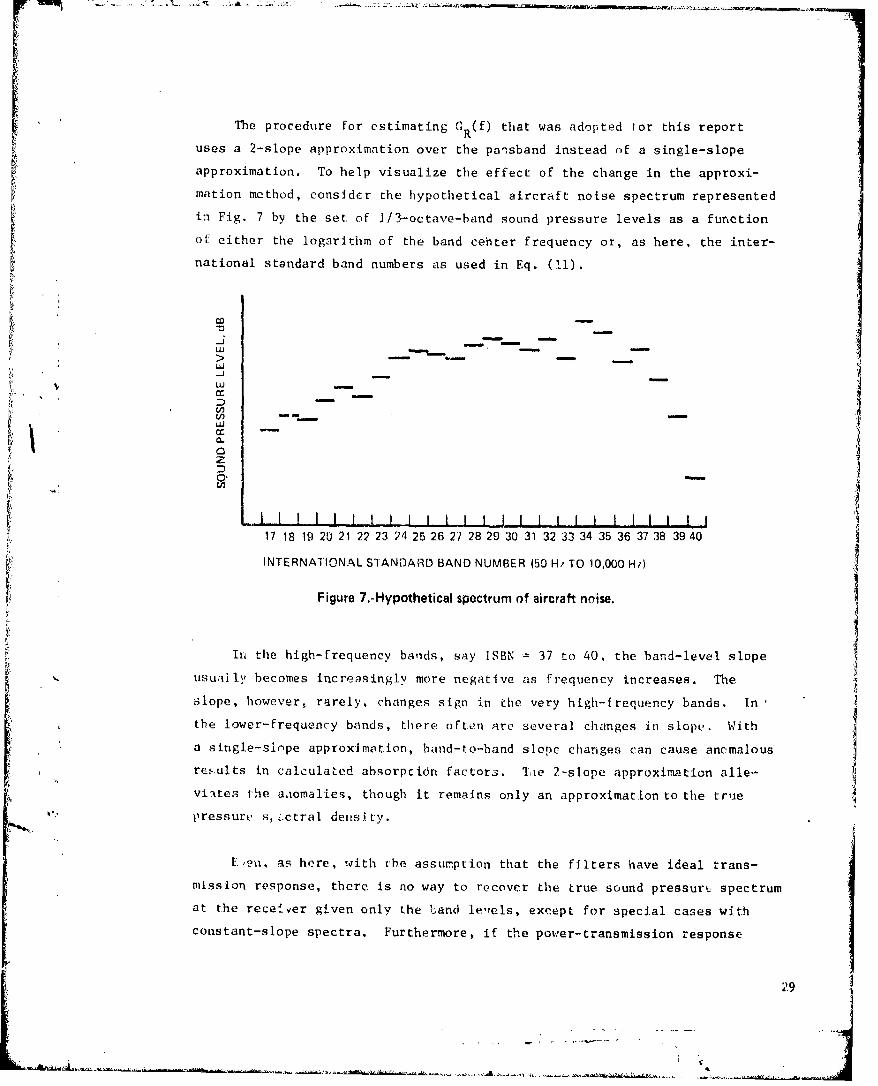
mation method, considcr the hypothetical aircraft noise spectrum represented
in Fig. 7 by the set of 1/3-octave-band sound pressure levels as a function
o[ either the logarithm of the band cehter frequency or, as here, the inter-
national standard band numbers as used in Eq. (11).
Co
)- -
Li
LU-
**- , IIL.,., I 1 1 I1111II 1 I I I
17 18 19 20 21 22 23 24 25 26 27 28 29 30 31 32 33 34 35 36 37 38 39 40
INTERNATIONAL STANDARD BAND NUMBER (50 H/ TO 10,000 Hi)
Figure 7.-Hypothetical spectrum of aircraft noise.
In the high-frequency bands, say ISBN = 37 to 40, the band-level slope
usually becomes increasingly more negative as frequency increases. The
slope, however, rarely, changes sign in the very high-f requency bands. In
the lower-frequency bands, there often are several changes in slope. With
a single-slope approximation, band-to-band slope changes can cause anomalous
reE.ults in calculated absorpcion factors. The 2-slope approximation alle-
viates the aaomalies, though it remains only an approximation to the true
pressure s, .:ctral densi ty.
Eei, ias here, with the assumption that the filters have ideal trans-
mission response, there is no way to recover the true sound pressure spectrum
at the receiver given only the Land le',els, except for special cases with
constant-slope spectra. Furthermore, if the power-transmission response
'. 2

* of the real filters cannot be assumed to be that of an ideal filter (i.e.,
if the filter's rejection rate is not high enough in the stopbands), or
if the slope of the sound spectrum changes rapidly with frequency, then the
filter frequency response must be considered in the calculation of atmos-
pheric-absorption-loss adjustment factors. In such a case, the problem
of estimating the true or actual spectrum of the sound pressure at the
microphone becomes much more difficult because there is no way to distinguish
readily between the effects of the ait;.osphere and the effects of the filter
on the resulting band sound pressure level. Re Ference 7 proposed an "Iterative"
method as one possibility. The "Iterative" method, however, would haverequired conqiderable effort to develop a practical implementation and was
i:not considered for this study. Add it Ionwal discussion of filter effects is
•) given in tile next Section.
Figure 8 illustrates the differences between using the single-straight-
line approximation method of Ref. 4 and the 2-slope method of approximating
the pressure spectrum. The examples are taken from the hypothetical spectrum
of Fig. 7.
lFigure 8(a) shows two canes where the band slope changes from negatIve
to positive over a band, Figure 8(b) shows two cases where the band slope
changes from negative to more-negative over a band. When there is a large
change in noise-level slope over a band, the spectral slope estimate based
on the difference in band level between that of the band above and the band
below the band of interest (i.e., the short dashed lines In Fig. 8) does not
yield a good approximation, especially when the slope changes sign as
around bands 33 and 36 in Fig. 8(a). When there is little difference in
band slope, as around band 38 in Fig. 8(b), the single-line spectral-slope
estimate based on the difference between the level of the band above and the
band below may be as reasonable as the 2-slope approximation.
When the pressure spectrum over the passband of a filter is approximated
by two straight line segments, the single integrals in the numerator and
denominator of Eq. (28) are replaced by the sum of two integrals ranging
from f"L to f and from f to f 1 In each frequency range, the pressure
spectrum, GR(f), is ai~proximated by a power function of frequency. The
30

MI
>
w
UJ
z0
34 35 36 37 36 39 3
1/3-OCTAVE BAND NUMBER
S(b) OVER PASSBANDS OF BANDS 35 AND 38,
(I
,-J
S~Figure 8.-Comparison of band-slope estimating procedures for certain bands fromhypothetical aircraft noise spectrum of Fig. 7.
.. .Band slope procedure of Ref. 4,... Band slope procedure based on lev'el differences in adjacent bands.
31
0. ,V •..

exponent for the frequency (the slope of the line segment on logarithmic
scales) is determined from the difference between the level of adjacent
bands. Figure 9 illustrates the process and defines the nppl icable symbols.
Note that at f = f G c(f C) C (f ) or a constant which canc RL c RU C R'C
be far'tored out and canceled from the ratio In ,q. (28).
Given these considerations the ratio of integrals in Eq. (28) is written
f +J U Q, Ic +FdV (if ) AF+d (F/C AF +dfNUMI + NUM2 (
J (f I)d + J. (f/f)1. C
L U 'where the pressure spectral density slopes, l and Z , are related to the
corresponding normal ized, non-dimensionat band-level slopes, SLL and SLU, by
LV = SITI - 1 (30a)
ki.ci' ~and!
9,1.1 = Lu - I ('iOh)
The normal zed band-level lopes are found from the differenves between
the sound pressure levels In adlacent hands using
SM, - II,R(f,) -L ,R(f )1/ O 10 lo (RF)) (31a)
and
silt] = ILR(f, ) - L,R(f 1 0) 1 l og, (R:)] (31b)
where LR(f ) relpresents the set of sound pressure levels at the receiver andc.
RF Is the band frequency ratio f U/f . For 1/i-octave hands, RF = 100
The, slope of the line over the lower hall of the first hand in the set
is assumed to he the same as that over the upper hal f of the first ba1nd.
Simllarly, the slope nf the line over the upper half of the last band is
assumed to he the same a'w that. over the lower half of the last band.
As for Eq. (22), the integrais In the two numerator terms, NUMI and
NUM2, In Eq. (29) were evaluated using the QSF numerical-integration subroutine
32

0
• ~GRU(f) --(GR(Ic) (f/fd)Vu
R (f/f:) 0) 1(GFOR fc • f < fu
FOR fL < f tc
fL. fU
Figure 9..Illustrations of straight-line approximations to sound pressure snectraldensity GR(f) with slopes kL and tU over passband of ideal filter withband center frequency fc,
33

d ld LIIi' 4110 hiiLcinclier ofi Irc'(piiitcv liIetvr;1h;ccc;c~ 111 vnccc I~ dcicr d c
prev I otis I yI
'Fbi' dunoml na tccr term s , * )N I andI I) N2 , I n I'q I' cev c v:, I I r)t v c!
d I rve c lIy . By a InalIcogy w ith[ t IcI.'o dVC' I Opmn 11 o 1t 0 VIN ( 12) 1n (I13) 1'or t Ice
evaluat I:ion of Eq . ( 3) , the (denoim nat or toeruns b~comle
rDENI = (f /5LA.)(1 - RPF ) (/ 32a1)
and
I)EN2 =(F~ /SLU)(RiP -L/ 1) (32b)
whei vil -1 (or SLL # 0) andIV ~- (or SIM1 0), rpet 'ly anrd
*lEINI = I)EN2 (1/2) In (10') ('33)
WheWII _ - I (or SLI., SIM1 - 0).
Wi th E'(s. (32) and (13), .cl te tins III Eq . (29) ec..I ho ca Itc a tod acid(
I i vd InI Elq. (28) to dolt.Ltittltit Lb.', aId ustmient factori to be added to the
h~and levvvto at the reeC'ivvr loca~lIon Lic give the est ima.t ccl band I ('Vo'! at
the sourcv . Compar loon WILII Owe k1Ic)Wn bind I eve ;it the So~irco provi deo
aI m1INIS IM' 01' the, avc oracy of the prowe~ss inid the aplpropr iat eness of the
app) rox I mat, I on o f the t riow p re4scire spec' L r;i I d(t011S It I.V
Ii gore 10 shcows tlhe reoci Its Hof ipp Iv ing, the method ove r I propaga tion
d IsHLalice 0of 600O11i and Fo r .c t.rut' -coI~ree-.Icand-I iVk1I s lope of - 121 dil/hand.
Stnt-t Iog WIith the recelver band leveok calculated for either 7(0 or 10-percent
1-e tailt I ye humid I ILy , thei app rox)% I 111i.c to me tHudlo I Heen to Ipriv WC aI very good
cm t Icicate of the t rute sour.'.' hand lee ov Is.
Figuire 10 atIouInd Icateo thc' true at tenuat.'I ion c'ausced by atmosplcer Ic
ab so rp t I oin over Lice 600-mn d is4t- anc e (ILS' - R 70or L,8 - L1R Ior thle 70 mid70 10
10O-pe rcvnt reI Lati ve hurn idfi t:y rond I t I mo) as well I ;s th livxac t t ust - t ()- rL'Ir-
ecrie-day adjusotment. factor 1I. N - L 0
'I1ic ncignIltuide cc0 the (IIIt erenrics 1Letween the exact and tiii. ;pprox imitt
source ba;nd level'!s Is olcown IiiII -g. 11 i I r the thcrev p~ropagaction di 0tanict.'
and the +1 and -12 dBl/hand Thop' '~e 1 ;rgest d11l fuirc'tices ocre III tlce lO-HlIv
'34

I -:•• -- • '- - --. • ".L .'. '. ,.• :.F • :: • . ;•.,. • _ .. ,.
190
170
150
130 -
. 110 --
90
r" UJ
ULJ 50>p
7J L. LS L R o-J 30 -
10 0 LS, TRUE, EXACT BANDCr •LEVELS AT THE SOURCE0 1• 0 (3 LR~o RECEIVER LEVELS;z FOR 70', RELATIVE HUMIDITY LS LRIo0 A LRo 0, RECEIVER LEVELS FOR
30 10% RELATIVE HUMIDITYLSo o, SOURCE LEVELS
50 - AL ULATED FOR 10' LR70 LRIORELATIVE HUMIDITY FROMLR10 LEVELS
70 - I)., SOURCE LEVELSCALCULATEL) FOR 70"..
90 RELATIVE HUMIDITY FROMLRo LF VELS
110B 1 0 1 2h 1 6 20 2 5 3 15 4.0 5.0 6 3 80 100 12.5
1 3.OC1AVE.BAND CENTER FREQUENCY, kH,
Figure 1O.-Example of determination of (1) attenuation, (2) accuracy of approximate band.integration method of calculating atmispheric absorption, and (3) exact band-lossadjustment factor from test (10% relative humidity) to reference (70% relativeL humidity) meteorological conditions. Air temperature is 25oc0; air pressure is 1.0standard atmosphere; spectral slope at the source is -12 dB/band; ideal filters;sound propagation pathlength is 600 m; no geometric spreading loss.* Attenuation by atmospheric absorption = LS - LR 7 0 or LS - LR 1 0 .a Accuracy of approximate method = LS10' 10 - LS or LS 70 ,70 - LS.* Exact band-loss adjustment factor = LR 7 0 - LR 1 0 .
35

717
U.,
Ul)C~ 4m -~
U,
(N
0
v ,on 6 E
(N
N
cuc~U tozW ý1
-j 0n 0 L
00400ae
(N .~ S
(6AKU3I IV S1A3 ONOI-ja~vnio133 0

hand, probably hbc'tiisv' or thle eXtrapoiatlion oF the sbtl( ovv'r the lowver
hal f ofr the hand to tie upper hal f or the band.
Neglect ig the di I F renten, In the iO-kIH'. band, tht, approximate metthod
i, seen Lo always give an evs LInnia eFor the source band level, that is either
equal to or mli;ghtly greater than the true source hand levels, the larger
diFrerenVes oc-urring For the much-more-absorptive 10-percent-relative-
humidity conditions, For the 70-percept conditions, the difference between
the estimated and the exact hIand levevvl wa never more than 0.2 dB and usually
.wa.u 0.0 il11. For the 10-percent humldity condition!,, the largest dif 'erenves
occu,,rreti In OWe ')-kll. h.ind but did tml ,xcetctc 1.4 (iM over the 900-111 1stan-.nt'e.
As a ma Itter o" in InLcr's•-L, Liht ra viut'l at ions oF source bancl level for allI
the cans shown in Fl Ig 1 weperlF-rmed twice, onltce wi.th the QSF
nomcer•ali-integration method and once with the ciosed-l'ornm-integral-stinnaiat. ion
nmethod Ol ReI. 4 reuprogramcnned For th is application., Identical results were
ob tPained Oa they W01r0 For tih c'alvculnLions of receeiver band levels.
ThieranL'er, ontly the QS F s,•uhre itInc was used for evalua1ting the integrals
In al 0 'u I at f tit ltenilitioc ovcer the propagation path.
Approximation of Source Band Levels byBand-Center-Frequency Method
The very good angrevcment Iin Fig. 11 between the e xact source hand
levev ln and nccourc'e bhand levc, l N es timated ustning Eqs . (27) and (28) was anti-
tci pated Iinvnece cretc lvi, r h;nd level.i hiad been talcculicted using Ideal
i'lltver, and the prc's.rure qpvlt'ral denstity at the recelver was closely
approximated by the two orinstanit-ni ope lines over the .lower and upper halves
of eavch passh•nd.
,intce. SAE ARP'Hl6A cis'n, csm•entlally, a bIand-c'eciter-frequency method,
"a natural quest ion wan how wcel woulcd a band-tenter-Freqoency method approxi-
in.cte i I a nt'enc|atlon over the propagat toil pa th.
Mhumo, Inlmead or cvi" oat l ag an integral tc det.tcrrmnu thet' 1ttVen1tatL.on
over the p:.thlength, [1c so-urce band levels were simply 'a lctcl;ated from
3 7

I,.•(l ) = R(f ) + 1. 1 1 ,)Ill I )
wihore a (I ) I is tilt' atLmosilie r I c :tl)sOrplt loll 4v, I I Ic Itti ;a(t li t, litind vt~ill t'Il
Ifreq (enity. Absorption coefficients were determinetd by th miet' t hod ol ANSI
S1.26-1978 at the exact band center frequencies determined from Rq. (11).
Comparisons of the differences between source band levels calculated
from Eq. (34) and the exact source band levels are shown in Fig. 12. Thedifferences are significantly larger than the corresponding differences inFig. ii for the band-integration method. Note that two different ordinate
scales were required as they were for Fig. 11.
Thl dlilerenc, e between L1t(e X~iC't sojitrce hand leyvel and Lhi, source hand
I levei extLI1Wted usi ng l.I, (04) IncreO,'1,s a8 Lthe slope of the sl)e('Lrum "it
hLit, reVci ev r [titc rases , I.e., as Ltiii source spec trum sl ope in ' roCses , ;v
Lhe propagat Ion d is tance I nC'',•ases, antd as t he a tmospic r I ( c'old I t Ions hecotuc'
more absorptive. The reason for tic is result is that the attenuatLion tit L Ite
bIattd-center frequency becomes a poorer ,and poorer est•imate of tihe trrue
attenua ti on as the slopt steepens beautse the actual atctteniat ion over the
frequency range of the filter passhand is determined by frequencies near
Lice lower bandedge frequency for steep, negative spectral slopes. The
true attenuation Is less at the lower bandedge frequency than at the band
center frequency. 'fxis obsrvaition Is the basis for the use in SAP ARP866A
of the nominal lower bandedge frequency instead of the nominal band center
frc(cltency for calcu]ations appl]cabte to the 5-kilz to lO-kHz bands.
'The results in Fig. 12 also indicate that if the spectrum is not too
steep, or the propagation itlstr.nc.e not too long, or the atmospheric conditions
not too absorptive (or not too differenti from reference conditions), then
the band-center frequency nieLhod Is capable of estimating the true attenua-
tion within I to 2 dB for band center frequencies as high ats 5 to 8 kHz
depentling on conditions.. The levels in the 5 to IO-kHz bands, moreover, are
often so low that they are below the level of the background noise and hence
cannot he measured with current Instruments. Thus, although not as accurate
as the band-Integration method, the band-center-frequency method may be
adequate in many practical situations.
.38
"..2
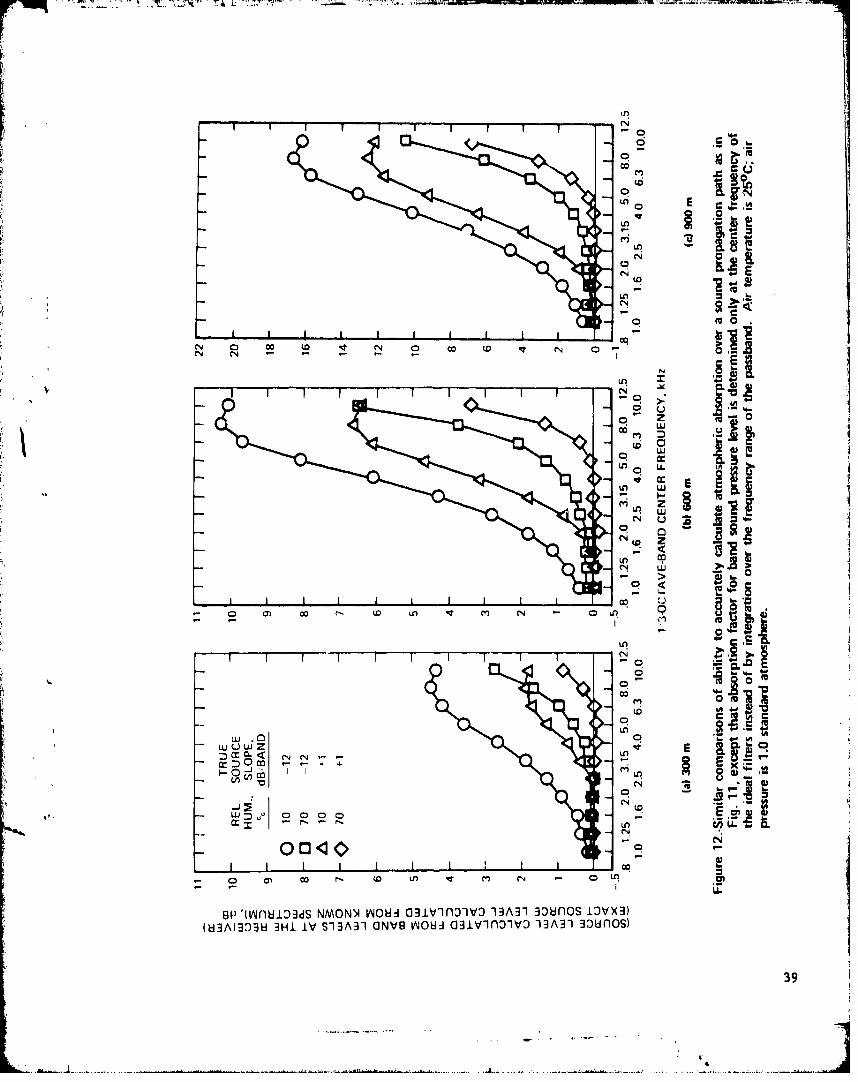
E-0 0E6
LA+ ,
00
- - -- 7
LA
CD
~LO ZUm zL
~NW -
N 0-4
00~~~~C to- 4 q
COC
WQWZ
(N
0 -
- c
LnA
co .i - §. E.
Approximate Test-to-Reference-DayBand-Level Adjustment Factors
Vie exact value for the factor to be added to the receiver band levels
for the iO-percent-relative-humldity test-day conditions in order to
determine what the receiver band levels would have been on a 70-percent-
relative-humidity reference day was found from the difference In the exact
values of the attenuation over the propagation path under the two atmospheric
conditions.
Thus, from Eq. (24), the exact band-adjustment factor can be written as
BA = att - att (35)exact lOexact 70,exact
- (LS - I'll (I'S - LR ) (36)exacte10'exact exact 70,exact
-LR11 (37)70.exact 10,exact
for the known, exact source band levels with the results as shown, in Fig. 6.
However, if we start with the exact receiver band levels for the simu-
1ated test-day condition, LROUexaLct, and calcullate the approximate attenua-
Liton over the path for [0-percent and 70-percent-rel[atILve-humI ldity conditions
in order to estimate what the source band levels would have been under the
two atmospheric conditions, then the approximate band-adjustment factor from
test-to-reference conditions can be determined. By analogy with the calcula-
tion for the exact band-adjustment factor, the approximate band-adjustment
factor Is found from
BA att - att (38)approx 10, approx 70,approx
= (LSlO,10,approx - LIZ 1),exaet)(HS0 - lllOea,)
- O'S 70, 10",pprox ll 1O'exact (39)LS - Is(40)
'V = Ll.O10 10,approx 1"370, 10,npprox
where tihlt subscript 10,10 means tlhalt thte source levels -re computed for
O-percent relative humidity starting from receiver levvls for a l0-percent-
humidity atmosphe.,re whllie the si.ihccrlpt 70,1.0 indicates source levels
calcul•atvd for a 70-percent humidity atmosphere but starting from the same
40

I;,AiraLc i rl, i'elur band pr, w s le ar t u l ( oi r a ii t ho,- I IO-I tar on-humldItv nd I Ii Ioni.
Ai.r tlumpol atr :turu Mild prt,!IsuL M'U COIrt, M (1:11 ; 01- '1l Cl ttl 101 10i|•.
Figure 13 presents an example of the calculat ton of approximate band-
adjustment factors for the same 600-m propagation distance and -12 dB/band
exact source slope shown in Fig. 10. Attenuation over the path was deter-
mined by the band-integration method. The magnitude of the exact and approxi-
mate band-adjustment factors is indicated for the l0-kHz band. The subscripts
approx and exact have been cmitted In the figure.
A measure of the it, ciracy ofi Ii Imetdhod of ihcminlt ing fg ratinOslph(,r H
absorption over a propagat• ton path is giveyn by the di fF'erenc•' between tih
approximate and the exact band-adJusttment factors, Eqs. (40) and (37).
For the example shown In Filg. 13, this difference is shown to be 1.1 dB itn
the 10-k[1z band.
Calculations of approximate band-adjustment factors and comparisons
with the corresponding exact band-adjustment factors were made for the
three propagation distances and for the +1 and -12 dB/band true source-
spectrum slopes. Attenuation over the path was calculated by the band-
Integration method and by the band-'enter--frequency method.
Figure 14 sutmmarzves the results of those 'al CIIIat lons. Th10 dat a in
Il g., 14 conf I ti Lhe trunds I-rom PlI gs . II and 12 wh lI h Ind Iated that the
band-integra t ion method provides a more-ac(Cu~irate cal cul at ton of at tenuat ion
over the path than the band-center-frequency method. Note that three
different ordinate scales are used in Fig. 14. Note also that the approxi-
4,mate adjustment factor Is almost always greater than the exact adjustment
factor; the small negative values shown in the figure are tile result of
round-off errors.
A summary of the range of the largest differences between the approxi-
mmate and the exact ad.justment factors is shown below for the two methods of
calculating attenuation and the three propagation distances.
41
. 1 A .. ".

7V
!!190 1 1 1 1 1 1 1-
170
5 150
130
S110"09
oir"
*0 70
LU6> 50
, -J
D 30 LS o, 10 LS1 QO LS, TRUE BAND LEVELL" AT THE SOURCEa: 100. ("3 LR70 , TRUE BAND LEVELSz AT THE RECEIVER FOR'D .10 70% RELATIVE HUMIDITYWf -/ LR 10 , TRUE BAND LEVEL-30 - AT THE RECEIVER FOR
10% RELATIVE HUMIDITY
LS•o 0, APPROXIMATE LR70 LR10-50 BANb LEVEL AT THE
SOURCE FOR 10%RELATIVE HUMIDITY
-70 •• LSo, 10, APPROXIMATE"p BAND LEVEL AT THE
---90 SOURCE FOR 70%RELATIVE HUMIDITY
- 110 ".8 1.0 1.25 1.6 2.0 2.5 3.15 4.0 5.0 6.3 8.0 10.0 12.5
1/3-OCTAVE-BAND CENTER FREQUENCY, kHz
Figure 13.-Example of determination of exact and approximate band-loss adjustment factors for* differences in atmospheric absorption under test (10% relative humidity) and reference
(70% relative humidity) conditions, Air temperature is 25 0 C; air pressure is 1.0standard atmosphere; spectral slope at the source is - 12 dB/band; ideal filters; soundpropagation pathlength is 600 m; no geometric spreading loss,
Approximate band-loss adjustment factor for receiver levels under 10% relative humidityis (LS 1u.10 - LSo 7 10 ). Exact band-loss adjustment factor is (LR 70 - L1R 1 0 ),Comparison of the difference for the 10 kHz band for this example yields'LSl0,10 - LS 70,101 - (LR 7 0 - LR 1 0 ) = (58.8 - (-58.1)) - (9.0 - (-106.8)) =
116.9 - 115.8 = 1.1 dB.
42

C,)C
E -
en-.
0
(N~~~C 0 5 0~~( Na* ~
- OPVN f0 ~ >-
Lo. .1()
r~ 0 _ 0 I
co E
L)O LL
ZZvC14
gN a
Ln 2)
1- 0
(V4 (5 E~ (N -0
Lq ~O ro r
m- - 4I FC6
0~
o -
C-i 4W

a at tenua n .. . . rLion6e - I . rges . i r ro I l.ca Ic itlatIloil MI. I tl .ngtl . III
method 300 f 600 900
,, integratIon 0.6 - I.I I 1. - 3.1 2.1 -4.8
center frequency 1.7- ).2 9.7 7.6 10.-3 12.2
k Thle error in the calculation of attenuation by the band-integrationmethod is larger For the +1 dB/band source-spectrum slope than for the
-1.2 dB/band slope, a result also shown in Fig. 11 for calculations of
source band levels.
lFor the band-center-frequency method, the error was larger for the
steel), -12 dB/band slope thar for the +1 dB/band, white-noise source spectrum,
Ia result which Is consistent with the trends in Fig. 12.
As a further observat.Ion from the results in Fi g. 14, we note that,
For a spec, ifled level of tolerable , accuracy, the band-tntv(-,r;itI()n m 'thod
Is abl I e to sat is fy the cr1terl on to h11gher I requen'Cleha s han(1 IS tIi band-
center-frequ oncy method for any comb in;•tion o.f prolpngtI•on dist:;ince and
source spectrum slopc.
As as final remark, we reiteratc the comment made earlier that although
the band-lntegratlon method appears, on the basis cf the analyses presented
here, to be generally more ac(uraLe than the band-center-frequency method
(significantly so in manv CaLmStx), the greater accuracy may be of limited
practical consequence when differences in atmospheric absorption are judged
in terms of psycdhocousttiC (10scrI•tors or time-integrated measutres such as
perceived noise level or sound exposure level.
a41,* 44

3. EFFECTS OF NON-IDEAL rII.TER CHARACTERISTICS ONCALCULATI ONS OF AI3SORPT ION-ADJUSTM[NT l'ACTORS
All I he anal yses Ini thu p rev i (01 See H on wert, per Iormed uinder(lt
'issulir1t ion that the 1/ 3-octavu-hai,c]I'll turs Ini tlwnhesrrmn systeml
at thc ro ce Iver Ineiat i on hlad the powe r- trans mis s ion- res ponse chn arc tkr is t i cS
of an ideal filter. A real, or pract teal, filter has response chioracteris-
tics that approach hocse of an idual filter. The most-Important difference,
for atrnospheric-ahsorpt ion anal yses, Is that the pract ical filter has finite,
rather than infinite, reject ion atL fruquencies in the stopbands below the
We examiline Some Of the e ffects, of iitn Ideal filter cha race 1ristices ait the
reveiver 00l aitmiosplier i e-alsorp it oni c'alculat ions.*
Filter Transmission Response
Ani ideal filter has a-r'I a-''t iVye power-IL rannmi ss filn ra 110 or power transfer
IutInc(t foil(!.o. ,te Irvat Io o I' Ie p )owe r t ransmItte L ;I t so me Frequtency to the
ciraetIIHCta pormttn the c xjrets ions for determining levels in thle
previous Sect Ion le . g., Eqs. (U) and (18)1 to be hinegrated only Over tile pass-
band f requency range from f to, f rather than ovur the infinite range from
0) t o i
lPract Ical 1 /3-cta~lVe-baini ff I turs (analIog or (Iigi talI) are designed to
comp I v wi th the CI ki.ss I I or GIlass I fI requirements of nat tonal F' and inter-
In-at I o 11; I stan lda rd(s. Class Ill re qu L re men t:s a re mo re sI:r in ge nt than
Class I I req Ili reenictits . Ve ry feow, I f any , class II I 1/ -or tave-band filt ers
A"tk are used to ana1Vl ~.e arcraf't noise nivasulremen ts. Miost, if not all, of the
I / 3-or Lave-hand fi lters cuirrent ly being, manufact uredl are designed It) meet
the ANSI , or I EC(, clos, I II reqjulrettients.
TheL (1,1I Is II I rfI-(1i IVcI'lut' spc siw Iv such proport les as thet exact, or
dcs ýIlg, hand -Venterfrrpeuv the tolerable ri ppl Itin thle passhand, the
re )cct Ioll rate ill t1e utophanlds , a-nd thle effective noise lbandwidth. The
01 FLfcct iWI y nise ad 1,Id JW(tll cit f'lueS the reltativye filter response at the lower
45

and upper bandedge freiquencies such that the filter will transmit the same
power as an ideal filter excited by a broadband electrical noise signal
having a whi te noiso spectri um.
tihe analyses in Refs, . 9 and 10 showed that the bandwidth error for
filtering of white noise was minimized when the relative response of a
practical filter was down 4.5 d(1 at th:e handedge frequencies with a pnssband
relative response of 0.0 dB.
Appendix 11 of ANSI Si.26-1978 contains a discussion of guidelines for
evaluating the atmospheric absorption Ios of broadband sound analyzed byI)ractlcnl] ft ltt, rs. ''Table F-I of Appendix , contains an equaLon which
app roxi ilhl tes, bilt is s1 ightitly lore conse rv;at ive thant, th:11 mlof tum translmis-
o ion-respons. re(qtiirements for a Class II I ff |ter. I1lie maxilmium transmission
respoilse Is thiat of an ideal filter.,
The eq(ti(t)ion for the rv i atVye power transfer function, 'i(f), from
TabLe E-T or ANST Sl.26 Is
T(f) h .4- h + (cl/r ) - (cr/f r - - (41)C V
and the corresponding expressiion for t:lho filter transmission loss, in decibel.-,
T(r) 10 1lop, Ii( )l. (42)
'lTIL' cool8 t ants a, ) , ani c In IFq (41) have spe cfic va1t ies applicable
to the frrequtency ranges dfitined for the stopbands and the passband. VaIlIes
given In Refs. 6 and 8 for h1 and c were modifled slightly in Table E-l of
ANSI S1.26 in order to satisfy the requirement for a transmission loss of
-4.5 dB at the exact bandedge frequencies.
1li, co t'ffic lents , ; Irv dofinled in Table E-I of ANSI SI.26 for Class III
coefficientIi I i i z tie(•ueiI y cL'Ifo a h C
owr otlophalnd: 0.1 8/I1. / /t 8/13 254 7 10-1/60
p;i bI.ih l(l: fl/ f/ fr .C f2/fc 1 0
upper sLophand:d f7/r < f/f < 10 8/13 2547 101/60
46. - - - - - 4
Z17 7. :7
where thie special frequencies f /f and f2f define the width of the O.O-dB
transmission-loss region for the pnssband. 'he special relative frequencies
have the values
f/f 10-1/ - 0.9261 (43a)
and
= 101/° 1.0798. (43b)f2/f
Ls I ng the vawl iie. for the toelI icfents •Ive.n iabove, Ole L ransml .sioll
I oss in the ,HLophand, at the rvl a IyV bandedge g requencivn 10-1 and
101(" [l'q. (8) - (00) ham the value of-4.47 dB (or a power t:ransmiission
rail.o of 0.357).
Figure 15 shows comparisons of the transmiss ion response calculated using
EqH. (41) and (42), the minimum transmission loss permitted for ANSI Class
Ii U'iltorH., and tih Lr.n' mIm ion response of an ideal filter. Figure 15(a)
preoent' Lh' colipartmon, on Ilogarithimi'c HC:ales to emphasize the differences
in the FILtur revpounses over the two decades of the ,it opband frequency re-
guionm, Figure 15(b) shown tLhe response on linear s'ales in order to
emtil)lha'ze the ditfferenices at frelquencies around thi spe('cial relative fre-
(iuenc'i e of Eq. (43) and the rvlatIlwV handedge -requm',n lem at f/f Ch .8913
and 1.1220. Equatlo)non (41) and (42) are seen to proyvide a good, omnewhnt
t'c)inet'vtivcy, predictLi on of the minimom ANSI CIass III requirements. Note
that the curve in Fig. 15(h) for the equation from Table E-I of Appendix E
of ANSI S1.26 crosse, the ideal-filter Line at a relative power transmission
ratio of 0.157.
'liThe po it (it thi, dl;'usi foil on ih;' been to clarify the differences between
ANSI Cla.so I II I/1-ottave-bhnd filter requirements, Idenl-filter response,n:di tie Ii Iter r('pon:•t pred'icted by Eqs. (41) and (42). The next issue is
ihow well Iloe.H the relponse of ac 'tual fi lters compare with the ANSI require-
11nIulL, or the predi.titonS Of Elqs. (41) and (42).
At the pres-ent t iMte, mO.t I/'1-ovtaive-band ;inal '.•,e of ni rcr;ift flyover
noise measuremenlts are made uslilng one orf Lhree models of' a real-time analyzer
having several conti[uoous [ilters In parallel: the Hewlett-Packard Model
47

• .- 10 - - - -
0
t I \I20
S-30 I-'J/
-40 -
z -50 -0
V 60 /
-70 - 7/ - --
80
-90 I
-100 0I0,1 0.2 0.3 0.4 0.6 0.8 1 2 3 4 6 810
FREQUENCY RATIO, f/fcla) TRANSMISSION LOSS, LOGARITHMIC SCALES
Figure 15.-Power transmission response of 1/3-octave-band filters.
-- -- Minimum TL for ANSI Class III; - Eqs. (41) & (42) 1 .- Ideal filter
48
-- - ---¢,- - --- ~-~-- -- - - ,,

•' ~1.0
0 .9 -
0,8 -
& 0.7-
z
0.6
0,5 I= IIw 0.5 --
,o.4 -
r',' I
0.3 - -
'i " I
0.2 -
iI
0.1-/ II
00.7 0.8 0.9 1.0 1.1 1.2 1.3
FREQUENCY RATIO. f/f
(b) POWER TRANSFER FUNCTION, LINEAR SCALES
Figure 15..Concluded.
49

8054A, the Gen Rad Model 1921, and the Brkiel and K.)aer Model Z131. Of these
three, the GR Model 1921 probably has been the most-widely used.
Response data on a representative sample of each .nstritment were obtained.
Design spec 'fication data for the (R 1921. were also obtained and compared
with the measured response data.
The 111) 8054A and the CR 1921 (which incorporates the GR 1.925 multifilter)
Use analog devices for the filters and, unless carefully adjusted, there
van be small differences between the response eharac teristics or indivldtia 1
liiterN in a set or' (o ot igL io 1is f llt ers as w e ll ns be tween dl lfforent fncl tru-
1'meats of the sa801 , Model . ThI& I K 21 II, however, ruses lIg t ,ila I I It erlng anid
;1 il rI l Lers In all Ins 1Lr ',ilnt i ; shio lId haive , tho same rspo nqtis cl ,thraIcter lI -
LIics .
F l igure 16 shows a compar isoil between typical f ilter-response data and2. -, the resp)onse ( 'il c tLI ited from E(is. (41) and (42) . In the lower-sto pband region,
ithe typical response data for al I three real-time analylers -Ire better (by
ais m uicti h as 7 dB) than the response oa .lc ul.'ated From Eqs. (4 1) and (42). For
the upl)er-stopl-and region, the typical response data are either equal. to, or
sl 1,,htly better than, the response From Eqs. (41) and (42)
Sinace the comparisons in l'ig. 15 showed that response C.alculated from
Eqs. (41) and (42) was slightly better than the ANSI Class I11 requirement,and since the typical real-time-analyzer f II ter-response data were sil g ,htIy
better than the calculat Ions oF Eqs. (41) and (42) , the actual practical
Filters must meet the ANSI Clhss 1I1 requirements. Also, the response of
an a'tfi i I / -oc tave-band Fil ter seems to be very well approximated by Eqs.
(41) and (42) ushla, the coefficIrents listed above. Thus, the typical practical-
liIter response a;Is predl 'ted from E 'qs. (41) and (42) was considered satis-
I.act'o ry Ifo r use In cal col at i tn) sou nd pressure leve ls a t the rece iver location .
50
- -- ----- ---.

-0
[3 GR 1921B 6& K2131
-20
F Il~ • ,
4-3
o
-30-40
-70.1.2 .4 .6 .8 1 2 4 6 8 10
FREQUENCY RATIO, f /I
Figure 16 6-Transmission- loss response characteristics of 1 /3-octave-band filters in realti me analyzers compared with response calculated f rom 'practical-f ilter'transmission-response equation; f'c is band center frequency.
51
ii• • -30 -L .
Spectra at the Source
In order to calculate the 1/3-octave-band sound pressure levels at the
receiver it was necessary to modify the sound pressure spectrum at the source
from that used in the previous Section.
11he power spectrum of the pressure shown In Fig. I would, theoretically,
apply to any frequency. For ideal litters there was no concern about contri-
butions at frequencies outside the pnssband hecause oi" thu Inl'Fnito reject i on
in the stopbands. A practical filter, howerer, can have significant contribu--
tion from the stopbands and therefore it was necessary to modify the low-
frequency portion of the source spectrum. There was no need to be concernedabout the high-frequency port.ion of the source spectrum since the high-fre-quency spectral slopes were all negative, or at most, flat. The decreasing
high-frequency pressure spectrum in combination with the decreasing high-Iifrequency filter response assured minimal., or negligible, upper-stopband
contributions.
Since From Figs. 15 and 16 the low-frequency part of the lower-stopband jresponse has aiin effective Hilope ofF about -7 to -8 dB/hand, any sound pressure
s pect rum that Increases In the lower-stlophand region o f a Filter by more than
+8 dB/band will. ultimately transmit. power Faster than the filter ran reol'rt
It. In such a situation, the power from the lower-stopband region can exceed
that from the passband. Tle converse, of course, could be true for the upper-
stophand region and indefinitely rising sound pressure spectra.
'To p)reserve a souise of realism in the calculations, the sound pressure
spect'ra of lI'g. I were extended down to the lower bandedgo frequency at one
band below the band centered at 1000 HIz, i.e,, using Eqs. (7), (9), (1.),
S;Ind (II), down to ;i frequency given by 10 • R '- - RF-°' 1" -0e '"07.946 liz.
,Below 10"' llz, the pressure spectra were maintained at a constant value
defined by the Vwl 10 of the pressure spectrum at 102,85 liz. A flat, low-
frequency pressure spectrum (rather than a decreasing ono) was selected because
many jet-powered aircraft have rather-flat low- and mid-frequency spectra.
Figure 17 shows the source -spectra that were developed on the bhsis of
the preceding analysis. The absolute value of the pressure spectral density
52
......... j

/ C*
(L IDLI-1
M CL'
-0 t.NW
N j Ix.
Lo .
--
cum U).
(0 C2 - Lm i
0 0~~
7, T.
at I00() 11Z has the same Value (106 iPa2/Hz) as used in Fig. I for the ideal-
filter calculations. The values of G at frequencies below 102"B5 Hz
are given on the figure.
The 1/3-octave-band sound pressure levels at the source, LS, are the
same as shown in Fig. 2 for the 1.1 bands between 1000 and 10,000 Hz. There
is no change in the true source hand levels because the actual filters
are considered •o be located only at the receiver. The true source band
levels are always Lhose that would be obtained with ideal. filters.
:•1.1Spectra at the Receiver '
I.gnoring, as In the previous SuctLion, any change in the amplitude of
t:hc sound I)ressure as a r,(stilt of sp read Ing the sourý-e ' s nct(ist ic power over
Incroasingly larger surfaice areas is propagation proceeds from the source to
the receiver, the band levels at the receiver location were calculated using
,he same basic Fourier transform relation as was used in Eq. (18) but inclu-
ding the filter power transfer function 't(f) from Eq. (41) and integrating I
over all positive frequencis.
Thus, with the response of a practical filter at the receiver, the
band levels are, theoretically, to bh found from,I. = 10 og )(44)
whter,, ,(C) is still rela;ted Lo the source spectrum G (f) [as defined insFig. 17) by 1'4. (17) and AF-(f) is still determined by Eq. (21) for uniform
atniosppher i c CO it ions.
The transmission response of a practical filter is defined, as noted
above, over the frequency range from f/f M 0.1 to f/f = 10.0. At thec,,
stopband limiting frequencies, the response is down approximately 94 dB (or
1 by a factor of 1.0 ) from the response at the band center frequency, see
F Ig. 15 GOa
Wi LIh t li o I IILtat ion oiu the Ir(qIten cy ran gv ol appl c (h I Iity associated
wIth the chloice of the definition of T(C) from Table El-I oi ANSI SI.26-1978
54 4

and making use of Eqs. (1), (17) and (21), the working expression for thesound pressure level at the receiver in some 1/3-octave-band can be written
as
aLR lo I[Cs(f )]/p 2 f}
LR 10 log
+ 10 log F/f M [df (45)
which can be compared with Eq. (22) for ideal filters.
The integral in Eq. (45) must be evaluated numerically. The 9SFnumerical-integration subroutine was again selected to perform the evalua-
tion.
One way of accomlplishing thIc evaluation would b1c to adopt the ;ipproach1 used In Ref. 3 and break the frequency range into three olarts: lower stop-
band, passband, and upper stopband. Each subrange would be further divided
into a number of intervals and the contributions from each subrange calcu-
lated separately.
Th le contribution in the passband from f /f to f /fc see Eq. (43),would be calculated first and used to define a reference vilue. 'lThen the
contribution from each stopband would be calculated -- that from the upperstopband proceeding from f 2 /f to f/f = 10, and that from the lower stopbandproceeding toward lower frequencies from fi/fC to f/fc = 0.1. The advantageof this approach is that the passband reference value can be used to definea convergence test which can be used to shorten computation time. At eachstep over the intervals in the stopbands the calculated value of the inte-
grand can be compared with a specified fraction of the passband reference
value (1/1000th of it, for example) and the calculations can be terminated
when an integrand value becomes less than the specified fraction of the
passband reference value.
Breaking tile integration range into three subranges and making use of
some type of convergence test would save'computation time, especially forthe upper stopbands where the absorption function decreases with increasing
55
]
A- r ~
fr(eqItincy for propogat lito I rol the I'(ii' lth- rcel vc'r Ind where t he ,o • tiud
pressure spectrum ftinction (f/l/ )' 'f also dt'c'rea se's with incrvias ig freq11ton 1 yC
for three out of the four vaw ues selected for P.'. The convergence test is
based on a predetermined judgment of when to stop the integration. The
Sjudgment is based on the assumption that the next, and subsequent, contribu-
tion in the stopband only provides a negligible amount to the total value of
the integral.
'l1e 3-sthrange/convergonce-tust procedure of Ref. 3 was not used to
evaluate Eq. (45) because the effort needed to define a meaningful conver-
goen e test would have exceeded the savings In computation cust. Also, for
110lily (C15e. u:XatiI Ietd here, the contrlbut Ion at suc('esslvi, steps over the lower
,t)lph;'1Itd h)O'am I sucC'e,,S , v by I r rger rather thLIn small ,r lecause the prIduct
(of the pressure-spectrum ftunctLion and tLhe ahorptlm function [nc2roasod
faster than the filter transmission lunction decreased. Indeed, for one of
the atmospheric conditions examined and for the hand centered at 10,000 liz
with a source slope of -12 dB/band, the value of the Integrand at the end of
the lower stophand at f = f /10 = 1000 tiz was larger by a factor ofC
approximately 3 x 10¹¹ than it was at the band center frequency.
The procedure that was adopted was thit s traightforward approach, similar
to thaIt used in evaluating q•q's. (22) and (29) , n which the entire fre-
quency ranoge, 10f - (f /10) , was just divided into a number of intervalsC 11
4 and the owmric;1al lot egr.t.ion by the QSF l iubroutine proceeded directly from
I. /10 to I10' lor each hand.
After soMe experime'ntation, the values tabulated below were selected
to subdivide the frequency ranges for the eleven hands. The frequency step-
sizes over the Frequency rang'e for any band are comparable to those used over
the passband frequency ranges of the ideal filters in the previous Section.
There are, however, 9911 frequenci es at which calculations are required here
for the 11 bands compared with 231 for ideal filters. The computation time
was on the ordur of 8 til ", longofr for evaluations of Eq. (45) than for
Eqi . (22).
56
-.-/ ~~i

Nomi na I Approx.band f req uenry Numb " fr
center ra n go S L VI)".IZ
frequency, lOfc - (c/ltO), inte Als, Af = range/N.Hz 1Hz N Hz
1000 9900.00 400 24.75
1250 12,463.36 500 24.93
1600 15,690.44 600 26.1.5
26000 19,753.10 700 28.22
2500 24,867.68 800 31.08
'3150 31,306.55 900 34 .79
4000 39,412.61 1000 39.41
5000 49,617.54 1100 45.11
6300 62,464.78 1200 52.05
800l) 78,638.50 1300 60.49
.10,000 99,000.00 1400 70.71
Some results arte presented in Figs. 18 and 19 to show the impact of
including the filter transmission response of Eq. (41) In the determination
of hand levels at the receiver. Figure 18 shows 1/3-octave-band sound
pressure level:- f ir tie 300--m pathlength and the 70-percent relative-
humidity (onditi,;5 Fig. 19 ;ll.,;,a shows data for the 300-m pathlength but
for 10-percent relalive humidity. OaLa for the four true spectral slope3
ill the source are included In each figure. For each source slope, com-
parisons ;irt shown between the exact source band levels, the exact
receiver band levels calculated with ideal filters, and the receiver band
levels calculated with the response of the practical filter.
In Fig. 18 for 70-percent relative humidity, there is little differ-
ence between the exact and the practical-filter receiver band levels for
source slopes of +1, -3, and -6 dB/band, except for the 10-kilz band and the
-6 dB/band slope.
For the -12 dB/band slope, however, significant differences start to
occur in the 2.5-kilz band and become very large in the 10-kHz band. The
practical-filter band levels exc'.ed the ideal-filter receiver band levels
57
•!: •=-: • .. .. :... ......... ... - -' • a... . • . .... . : _ • .. .. .. .. ,e•.......... ........... . ..... ,......• ...

190 "- 190 I1 "
o 180 - 180
' 170 170
1 bo 160-J
cc 0 LS, TRUE BAND LEVEL:D 160 - AT THE SOURCE 140uJ 1"3 LR70RECEIVER BANDM : 140 -- 140
a LEVEL, PRACTICAL FILTERz
130 70 RECEIVER BAND 13CLEVEL. IDEAL FILTER
120 120 L J I I I I.8 1.25 2.0 3.15 5.0 8,0 12.5 .8 1.25 2,0 3,15 5.0 8,0 12.5
1.0 1.6 2.5 4.0 6.3 10.0 1.0 1.6 2,5 4.0 6.3 10.0
1/3 OCIAVE BAND CENTER FREQUENCY, kHi,
(a) SLOPE + 1 dB/BAND (b) SLOPE = -3 dB/BAND
Figure 18,-Effect of filter characteristics on band level at the receiver for variousslopes of the sound pressure I..,,el spectrum at th. sourr~e. 300.ra sOundpropagation pathlength; 70 % relative humidity; 2.', 'C aie temperatuie;1.0 standard atmospherc air pressure,
58
~, 4 I

180 180 1
S170 - 170 -a-
S16o- 160 l
S. 150 - 150 -; >,LUJ
.-j 140- 140ILlM
130 130Lii
•120 120Z
110 110
100- 100
90 90
80
.8 1.25 2.0 3.15 5.U 8.0 12.5
1.0 1.6 2.5 4.0 6.3 10.0
30
S1/3-OCTAVE HAND CENTER FREQUENCY, kHz
(c) SLOPE -6 dB/BAND (d) SLOPE - 12 dBIBAND
Figure 18.-Concluded.
59
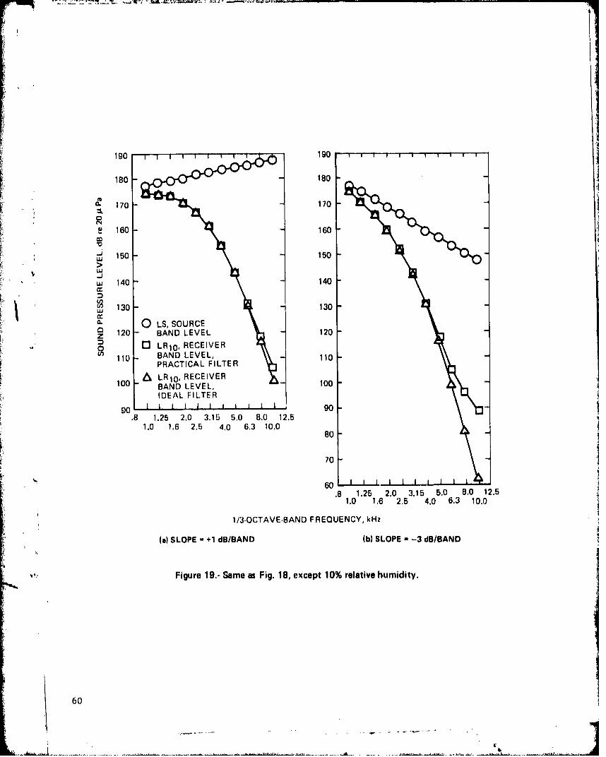
180 180
170 -170
160 -160
L 150 150
wj 140 140
U 130 130
0 LS, SOURCE120 - BAND LEVEL 120
0LR10, RECEIVER110 - BAND LEVEL,10
PRACTICAL FILTER - 1SLR10 , RECEIVER
100 BAND LEVEL, j 100IDEAL FILTER
90goI i i 90.8 1.25 2.0 3,15 5.0 8.0 12.5
1.0 1.6 2.5 4.0 6.3 10.080
70
.8 1.25 2.0 3.15 5.0 8.0 12.51.0 1.6 2.5 4.0 6.3 10.0
1/3-OCTAVE-BAND FREQUENCY, kHz
(a) SLOPE =+1 dB/BAND 1b) SLOPE - -3 de/BAND
Figure 19.- Same as Fig. 18, except 10% relative humidity.
60

180 180
t 160 160
,N 140 - 140 -
120 - 120
w100 - 100
w~LU
x" 60- 60 -0z' 40 - 40 -
20, 1 11 20.8 1.25 2.0 3.15 5.0 8.0 12.5
1.0 1.6 2.5 4.0 6.3 10.00
iK -20
-40, 1 1.8 1.25 2.0 3.15 5.0 8.0 12.51.0 1.6 2.5 4,0 6.3 10,0
'cS 1/3-OCTAVE.BAND CENTER FREQUENCY, kHz
1c)e SLOPE '-6 dBBAND (d) SLOPE -- 12 d/BAND
=• Figure 19.-Concluded.
I ~61

and indeed even exceed tile source band levels! In the l0-kHz band, for
example, the practical-filter receiver band level exceeds the source band
level by about 20 dB and the ideal-filter reei.ever band level, by about
45 dBl.
For the highly-absorlptive 10-percent relative-humidity conditions of
Fig. 19, the situation is substantially more critical than it was for the
70-percent reference-day conditions of Fig. 18. Note that whereas it was
feasible to use an ordinate scale with lO-dB per major division for all
plots in Fig. 18, It was necessary to use both l0-dB and 20-dB per major
division in Fig. 19 because of the much-steeper slopes over the lower stop-
Sband under tile more-absorptlye conditions.
As the source spectral slope bec'ame more and more negative, the devia-
"tLion between the practical-filter and the ideal- filter receiver band level
occurred at a lower and lower frequency: 6.3 to 4.0 to 3.15 to 1.25 kHz
IS tile sourcet slope chAnmged from +1 to -3 to -6 to -12 dB/band.
For citmpirIson with Lilt, exampl c qluoted abovr, for the 70-percent
condition, th, --12 dI/band s lope data In Fig. 19 show that the practical-
fift1 r rtcc I vr c band leveI in the 10-ktlz band exceeds the source band level
hy •bouit 19 d( buht exceeds tie cXli ec reclver band level by 104 dB compared
with 45 dBi in Fig. 18(d).
The message from these results is that high-frequency 1/3-octave-band
sound pressure levels, iiie;,,ured at a receiver location with a filter meeting
the most-stringent ANSI requirements, may differ from the expected band levels
by g ignt icanlt amounts, dhpend fo, (o1 how steep was the si ope of tihe spectrum
(It' 1110 nIS so 'e adll l h I)w qbtopt L[Vy wIs the atmospherc .
fThe reStuls in FI gs. 18 and 19 showed tile e'fect on the band levels at
Lilie t '' L1 irciw rea ii i1 thle spveelttra•1 slope at tile source for a fixed
ct'paig~lt (oit bice Of 300 "1. If the propagation distance were to be
inctretased, thlen similar, but more-pronounced, trends would be expected.
62 :t

Figures 20 and 21 present vomiparisons in the format of Pigs. 18 and
1.9 for propagation distances of 300, 600, and 900 m. Figure 20 presents
results for a source spectral slope of +1 dB/band, Fig. 21 for a slope
of -12 dII/band. Each plot In Figs. 20 and 21 Includes the band levels at
tile source and the band levels at the rec'elver for 70 and I0-percent
relative humidities and for Ideal and pract ical I/'3-oetave-band filters.
For the +1 di/b;ind-slope results in Fig. 20, there was no significant
difference between the exact receiver band levels and those with the prac-
tical rilLer when the atmospheric aItsorptLon had the minimal values
associated with 70-percent relative humidity at 250 C air temperature.
'lThe Iirgest differencewas only aboul 8 (B in the 10-kHz band for the 900-m
K * " path.l.ungth
Vor the lO-percent relatilve-ihuncidty, highly-absorptive atmospheric
conditions, however, there were large differences between the exact and
the l)r'cI ical-fiLter receiver band IeVwis. For a given hand center fre-
qtuency (e.g.., 1.0 kili), the dlifl'erence Increased ts the pathilength increased.
The I'rel(jUency, at whtich the di ference between Lhe exact and the practical-
fitlter band levil firs t beco'tes significant, decreases as the pa thlength
in- rvi.P.H
For Lihe 10-percent re ulative-hun|ldiily data In Fig. 20, there appeared
to be a saturation-like effect that occurred for the high-freqi.ency receiver
band Ieve I; for the 600 and 900-m path lengths. Apparently, the power
transmitted through the lower stopband becomes more and more the control-
ling factor in the total power transmitted as the absorption function
steepens with increasing pathlength. As an example, consider the l0-kilz
band where the practiCal-filter band level only decreased about 8 dB for
the 10-percent relative-humidity conditions between the 600 and 900-m
pathlengths. The correspondting difference in exact band le.vels was about
82 d1B. For the 70-percent concditions, the receiver band level decreased by
I18 ind 24 d!1O ior tilt, prac ltcal and ideal i-ilters, respectively. Thus,
tie lewV I for the 10-percent condition should have decreased by much more
than 8 ll.
0,"
_......
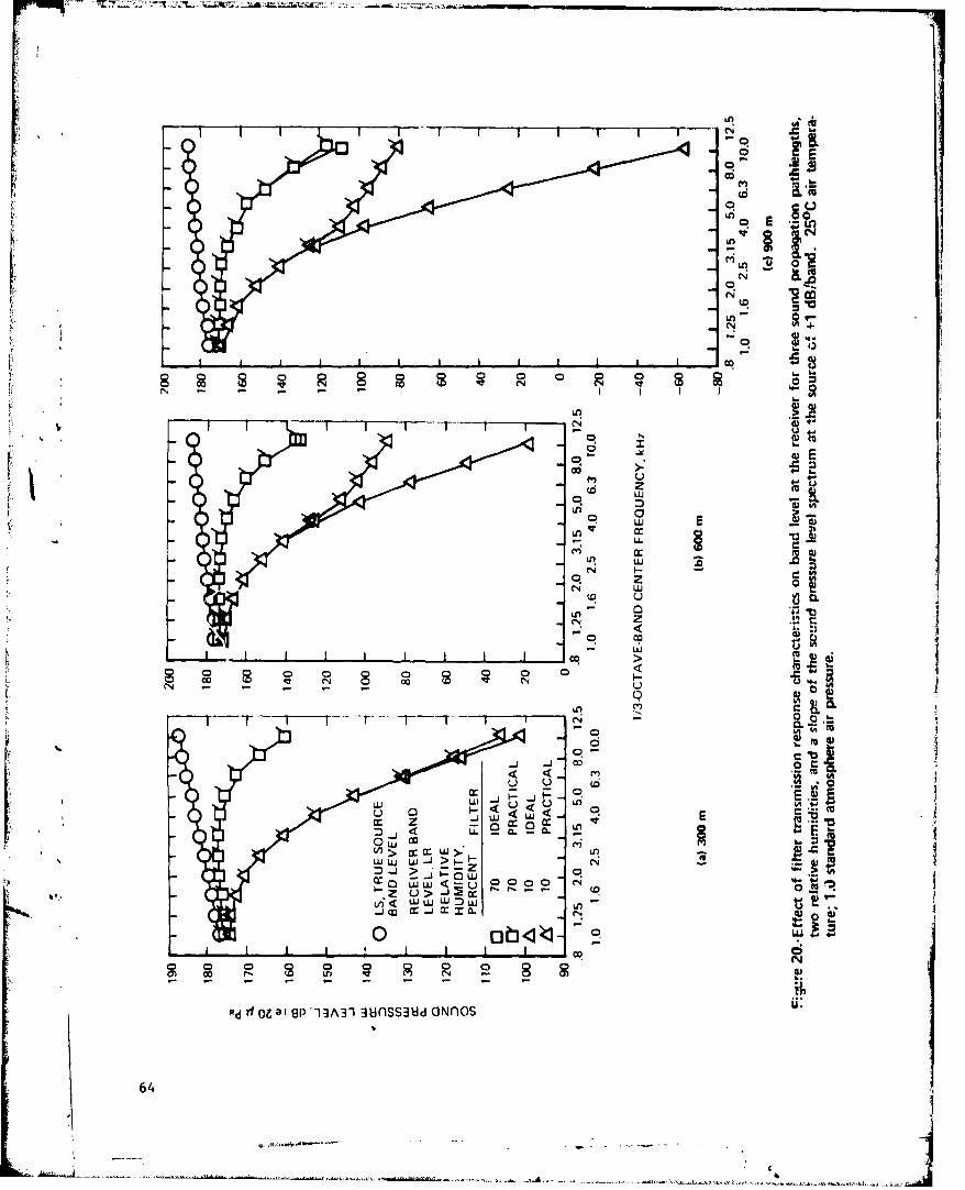
-o oN
0n
CN
NO 01
-T- N
00
Ln
~ WUJ.Jflw.~ II.. Hn ~ a-c0
64W
Nj

C14
L0
00
N~~U( C1 .4c N
NN
i 4w
00
0 J
on wNU, U
0~CL
to w
(N 0u
0) 0 0(N c- N - I
-7 ----- --
Uc 0oUJU
[II
(N -J - > ND >cr ui C65
Lu <5u-.- ~. .. .-- ~.- - - U > 4c

It is noted that presumably valid measurements of aircraft flyover
noise spectra for relatively absorptive conditions have been reported which
have a high-frequency "tall off" simil ar In appearance to those shown In
I11 g• . 20(b) and 20(c) fo r the 10-pereent relat vye-hum1idlty condition. 'TIhi,
suggestl I on Is that the reported I evev 1 , whi I ci were sa id Lo be we I I above
the L'orrespond Ing background no I se I eve Is, may not be val d because of
contamination by power transmitted through the lower stopbands of tile prac-
tical filters used in analyzing the tape-recorded signals.
'iThe results presented In Fig. 21 show additional evidence of a satura-
tion-like effect when the source slope is -12 dB/band. The receiver band
levels, as in Figs. 18(d) and 19(d), are higher, instead of lower, than the
"source band levels in the high-frequency bands. There was essentially nodifference between the practical-filltr band levels for the 70 and the 10-
percent conditions for any of the three pathlengths. In contrast, the differ-
ence between the exact rUceiver band levels for tile 70 and 10-percent c'ondi-
utions was large,, as expectLd, and Itp.creasod as tihe pathlength increasod.
Note that an ordinate scale with 40 dIR per division was required for the
data in Fig. 21 compared with 10 or 20 dB per division for the data in Fig. 20.
The inference drawn from the data in Fig. 21, and from the comparisons
in Figs. 18 (c), 18(d), 19 (c), and 19(d), is that once either the receiver
spectral density function, or the absorption function, or their product,
starts to increase faster than the filter lower-stopband response decreases,
"is thle Integration proceedn from the passband toward the lowest defined
frequency at f /10, then the band levels at a receiver location which wouldCresult irotm using a practical filter meeting ANSI Class IIt requirements
will he higher than the expected or exact values and by very large amounts
for soiiie conditions. Indeed, if, as in Fig. 21, the source slope is as
stecp as -12 dR/band, then the receiver band levels indicated for the
response of a practical filter can become essentially independent of how
Sahsorpt Lyv the attnosphere Is or how long the propagation path is. There
werc, diffe rences between the pract Ical-fil ter receiver band levels for the
70 and iO-percent conditions and for the three distances, but they were small
and are hard to see with a 40-dB-per-division scale.
66 J

•Two corollaries follow from the above inference. The first Is that
aircraft-noise dato-i-nalysis systenis In currnt liSt, mi:v not hIo ,lt, it1
provide me.aning ul. nfci .,lL' suronL',llleut i hi gt l i-qIreq il'v i I / 1-,tetl;iv,-bh.nl o liltd
pressure eo vvlts If the nI OsoeH iiir ce spote'trum Is tooi stoep, or the, 1t11iot.14-
phere is too absorptive, or the propagation path too long. The second is
that attempts to use measured aircraft noise 1/3-octave-band sound pressure
levels to derive, or verify, the high-frequency absorption characteristics
of the atmosphere may not he feasible and could lead to incorrect conclu-
sions.
SThe differences between the practical- and ideal-filter receiver band
levels could also affect the validity of attempts to adjust measured data
from test-to-reference conditions, as well as attempts to use measured
*iaircraft noise data to vatlidate or develop airc,rerft-nosle-predcl'tion methods
or to Jtlge the elffectivenoss of high-fre(quency no l.-suplpresslon device's
in1 L.1 i ed I inan lnly I 1C. Ana il ,lv Le, ( I nool Inear propagait lon iItfet ;iald the
cO flectLs o f aL4n ctlher ic ttll tli)U cIol l o soind p ropaglat: in may ailso be L l-
enceed by the use of Iracttical-f iter band levels that aire hitgher than the
corresponding ideal-fIl.Ler band levels.
The potential problems introduced by the response characteristics
of practical filters as well as possible solutions, would clearly seem to
be areas dese rving add it ional study.
Test-to-Reference-Day Band-LevelAdjustment Factors
Although the I'CSUt] ts were expec ted to be much different than those
cbhtaind using the exact or true band levels at the receiver, it was
considerud that it would be InstructLive to use the receiver band levels
calculaLctd for the response of a practical I ilter In determinations of
band-level adjustment factors from test to reference atmospheric conditions.
Determinations of ad cistment factors wotild use the analysis described
in the previous Section. '[hUt "measured" band levels would be assumed to
have the values that would have been obtained with ideal filters. Integra-
67
- - - -.- r -.-
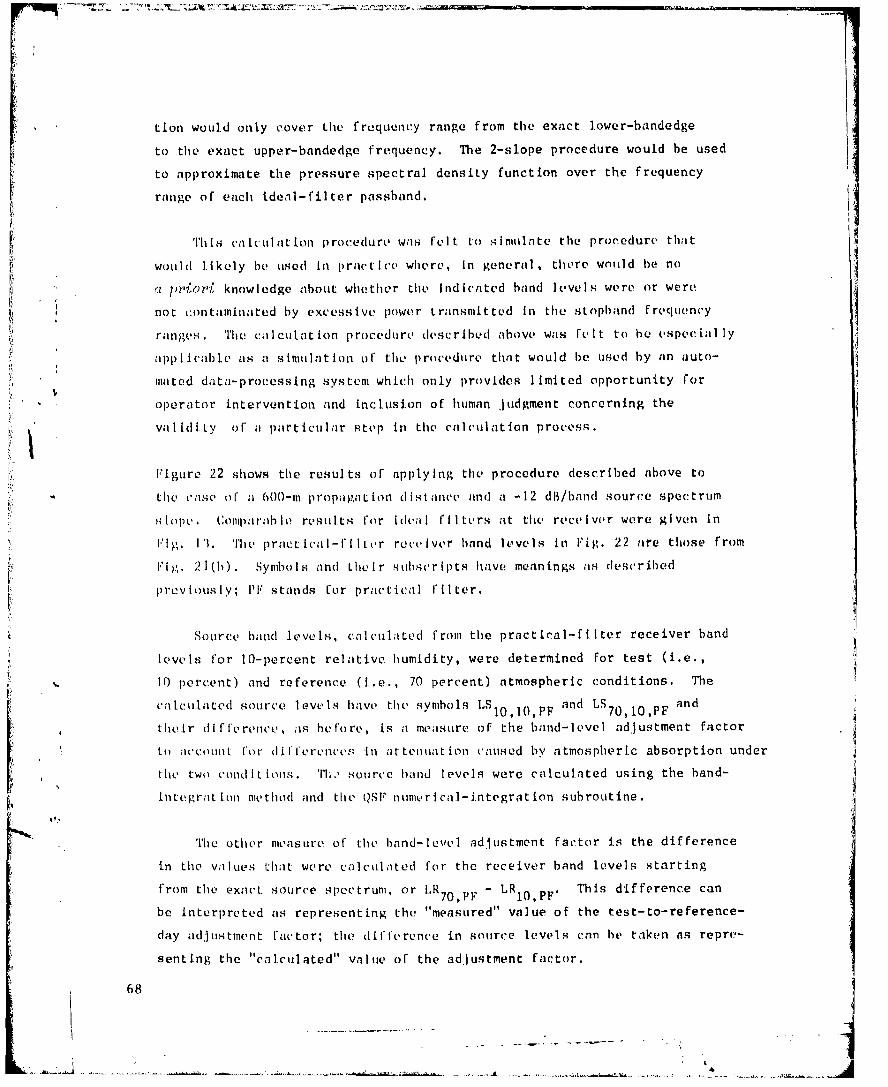
lion would only cover the frequency range from the exact lower-bandedge
to the exact upper-bandedge frequency. The 2-slope procedure would be used
to approximate the pressure spectral density function over the frequency
range of each ideal-filter passband.
I'This calcul ation procedure was felt to si nuilate the procedure that
WOuld likely be used in prract lce where, in general, there woold be no
a" pmiori knowledge about whether the Indicated band levels were or were
not montaminated by excessive power transmitted In the stopband freqiency
ranges . The cal culat ion proceduire discribed above was fe It to he espec ial ly
applicable as a simulation of the procedure that would be tused by an auto-
mated da-a-processing system which only provides limited opportunity for
F "operator intervention and inclusion of human Judgment concerning the
valid 1.ty of a particular step in the calculation process.
Fligure 22 shows the results of applying the procedure described above to
the case of a 600-m propagation clist ance and a -12 dB/band source spectrum
H lope. C, omparablo resul.ts- for Icea|i rliters at the receilvwr were given in
FI.g. 11. The practical-fIltr receiver hand levels in Fig. 22 are those from
I"1:,. 21(h) . Symbols and their shubscriplts have meanings as described
previously, IF stands for practical filter.
Source band levels, calculated from the practical-f, Ilter receiver band
levels for 10-percent relative humidity, were determined for test (i.e.,
10 percent) and reference (i.e., 70 percent) atmospheric conditions. The
caLculated source leve ls have tie symbols IS and LS andl10,1)PP 70,1O,PF
their difference, ais before, is a measure of the band-level adjustment factor
to aiccount for diiIlerences in attentiation caused by atmospheric absorption under
the two condMit ions. ThI. source band levels were calculated using the band-
integraLion method and the QSF numeri cal- integration subroutine.
'111e other measure of the band-level adjustment factor is the difference
in the values that were calculated for the receiver band levels starting
from the exact, source spectrum, or LR70,PF - LR oPF. This difference can
be interpreted as representing the "measured" value of the test-to-reference-
day ad)justment factor; the diil'l'e rence in source levels can be taken as repre-
senting the "calculated" value of the adjustment factor.
68
i~~~ . ..... ... . .. .. ...

260 1 I I I I 1
240
220
20020LS10,10,PF LS70,10,PF
i:1.0 180
S.. .. "• 160
-J
> 140UJ
uJ 0 LS, TRUE BAND LEVEL* 120 - AT THE SOURCE
0 LR7 0,PF BAND LEVEL AT
r 100 RECEIVER, 70", RELATIVE"C. HUMIDITY, PRACTICAL FILTERZ LR10.PF BAND LEVEL AT
: 80 RECEIVER, 10% RELATIVE
HUMIDITY, PRACTICAL FILTERULROFLlOP
60 -. ( LS10 10,PF APPROX. BANDLEVEL AT THE SOURCE,10% RELATIVE HUMIDITY,
40 PRACTICAL FILTER
LS70,10,PF APPROX BAND
20 LEVEL AT THE SOURCE,"70% RELATIVE HUMIDITY,PRACTICAL FILTER
0 1 1 1 1 1 I I I I0.8 1.0 1.25 1.6 2.0 2.5 3.15 40 5.0 6.3 8.0 10.0 12.5
1/30CIAVE BAND CENTER FREQUENCY, kHt
Figure 22.-Determination of band-loss adjustment factors when band levelsat the receiver location are calculated with the filter transmission-response characteristics of the practical filters from Fig. 15; comparewith results for ideal filters in Fig. 13.25 0 C air temperature; 1.0 standard atmosphere air pressure;-12 dB/band spectral slope at the source; 600-m sound propagationpathlength; integration method for absorption loss.Band-loss adjustment factor from levels at the source(integratingover passband of ideal filters) is (LS10,10,PF-LS70,10,PF).
Band-loss adjustment factor from levels at the receiver is(LR70,pF-LRoPF).
Difference here, for 10 kHz band, is (250.2-129.9)-(77.0-74.1) =
120.3-2.9 = 1 7.4 dB.
69

Using the O0-ktlz band for an examplo,, as belore, (lit, resutlts in Fi)g. 2
indicate thit the difference in calcu.lated sou.rc.e, levels is a reasonably
accurate measure of the true difference in atmospheric absorption under the
two conditions. From the data in Fig. 22, the difference is LSl1lOPF
"- LS 7 ,IOPF 250.2 - 129.9 120.3 d13 compared with the exact value of
115.8 dB from Fig. .13.
The adjustment factor determined from the difference in practical-
filter receiver band levels is much different than the difference in source
levels because of the lower-stopband contamination problem. ITlus, using
data from 1'1g. 22 7 P1 77.0 - 74. 1 2.9 d( in the l)-kllP band.io ' 70, P" VO, PV"
llicre lore, I11 the Prr;tical-Fller "inveastired" receiver hand leveIs forU'
Lest ;ind tlccICretCe (cOnd itIolls wrve to be used to assess the ;ccuracy of
dct rnii ing band-level ad~justment Factors, the results in Fig. 22 would c
Irdicate a huge error. in the 10-kilz band, the above calculations indicate
that the error would be 120.3 - 2.9 1.17.4 dB for the 600-m pathlength and
-12 dB/band source spectrum slope.
In additloti to the extreme value of the calculated error, use of the
contaminated pract tcal-filter receiver band levels to estimate the source
levels results in a severe distortion of the true shape of the source
;peu rI L1o1 acid exceedingly large indi cated source band levels as shown in
I"'ig. 22. It Is noted that calculations of "source" spectra have appeared
in thW I literaLture with shapes very similar to those shown by the LS
;and I'SlO, 1OPlc spectra in Fig. 22. The suggestion is that, although the
clc;clc.ulatcd at tenuation caused by atinosppheric absorption may be approximately
correct, the adjustment factor has been applied to contaminated, or in-
correct, receiver band levels.
To coipleteLI the annlvsIs of teist-to-reference-day band-level adjustment
li ctors as app lied to sound pressure levels at the receiver which were
.(Letermined using the response curve of a practical filter. it was decided
Lo examine tle differences between the calculated source band levels
(OS IOIOPF- I.sTOIO.PF) and the calculated receiver band levels
(LR 70,PF - , RIOPF). Analyses were carried out for the two source spectral
70

slopi s of +1 aid -12 dil/btnd -d for the I hrce propj;gai (on distanices (i1'
300, b00, and 900 m. As In Section 2 f or the analyses using Ideal
filters, adjustment Factors were calculated by ihe band- integration
metho" and the band-center-frequency method for the eleven bands with
center freque frrnm 1000 to 1O,000 lHz.
Figure 2'. shows the resulis of the analyses. Comparable ideal-
fItlte results were presented K' Fig. 14. Note that the ordinate scale
in Fig. 23(u) is difft 'it frm, Vcim in Figs. 2 (Wa) and 2 3(b).
Th " rror" L c in 'c cl ual;Ict. i f o f I:e I band-iv'Il acd just:mvnut ftactior
I s seen t-o L'. s[1;1 1 4 ), I,, ), 11),, 1 e ] (I r m 00 l()O Iz io ,somu, I*rvquenc-y an1d( t hon
to i:l('rca;v• very rapildly. Thbv larg,,sL vrrnws In Flo. 21 are [).gger by a
factor ofl 15 to 20 than th, Ilargt'st errors in HIg. 14 for receiver levels
calculated with FMiters li vitn g ideal response charac Ic ristics . The
Frequtency where the c mro 'tart:s to increase corresponds to the frequency
where Lh,, practi'a l-Filter rec'ivwr band levels start to deviate from the
Idoal-filltr receiver band levels as seen by comparng the results in
]"t;•s. 20 and 21 with the error analyses in Fig. 23.
Aside from the difference in the shape or the curves and the very
large .ri[Ftrence In the mignILtde oF the rt'sulIs,, the other ma]jor differ-
onve between ticP' idtani-Fit:,or resulL Isn iFJig. 14 and the practical-
I Ilor resuiLs in fIg. 23 is that in FIg. 21 tcie "et' rror" In calculating
tIii bhand- adj ustlment F c'Lcor is somncewhi at largeur by the hlnd-integratl(on methodthan by the hand-center- frequcency melthod. The reasons lie band-center-
Frequency method gave relatively sma]ler indications of error than it did
in 1F'Ig;. 14 Is probably 5 eca,itise tht spectrum of the sound pressure at the
re'eiver, thati wa, cal culIated for the pracctical filters, Is signinficantly
less steep than tie spectrum ca lculated using Ideal F i lters, see Figs. 20
and 2 I.V'lic dFfferences shown in Fig. 21 between the two methods are not
,egarded as significant, however, because the basis for the comparisons
(the so-called me;sured adjustment factor or difference between reference-
day and test-day receiver band levels) is obviously not correct in many
bands as can be seen by inspection of the data in Figs. 20 and 21.
71
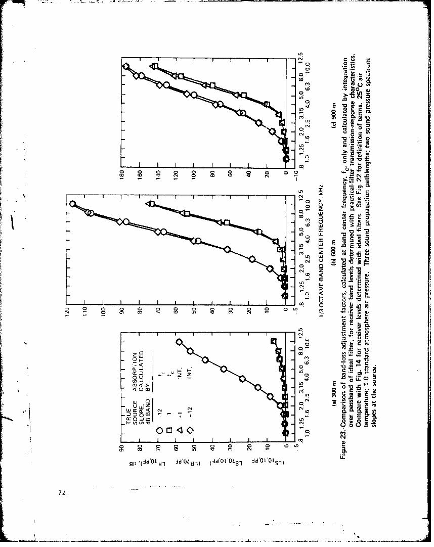
L4ALn T
LO
0ý0
Ln c
0 00C00o 0T 88 00ti C
UN N -
00 4- V
0)
q cc
LC cr4 L.
(0 w t
u
00
LO
Lj 0L E
000
LA C
(00
-n E -
DCo 03 8 E L
0 1' c~oL~ dLl ~'~Os dO~s
8

A -A
Thus, it is considered that the conclusion of Section 2 is still valid
wi th regard to the accuracy of the band-integration and the band-center-
fr&,(luen('y methods: namely, that when the band I,,ve ls ;it tiht rece, [ y r ;ar
prop, rly deteri|lined, the haind-Intgr;atlIon methoid Is ;preferre, d httiset, I I
produlces simailler errors for stoeup, negative, high-freitlen('y spectr'la
slopes than the b;ind-ont, r- frequen(y method. For moderate spec t ral slopes,
however, there is no signific'nt. difference in the accuracy of the two
methods and either one can be used equally well for determining band-
adjustment fa'tors.
IIThe crtitical issues It1 the choice of cal culation method seem to be:
how accurately are the correct receiver band levels known and, for the band-
.p integration method, how aLccuratelv does the 2-slope method, or some other
method, approximate the presser(, spectrum of the sound at the microphon".
As a practical. matter, there does not appear to be any feasible way toUresolve these issues. The next Section provides additional guidance asI ;L result of applying the anl.lytica.l procedures to nctual aircraft flyover
no ise icas ureme nti s.
7 .
73J
-is

4. ADJUSTMENT OF AIRCRAFT NOISE DATAFROM TEST TO REFERENCE
METEOROLOGICAL CONDITIONS
Thu objectiLve of the second phase of the study was to make a nuant I tati lye
evaluation of various procudures to adjust measured aircraft flyover noise (d.ata
for differences between atmospheric absorption under test and reference meteor-
ological conditions. A primary application for such adjustment procedures
would be during analysis of data taken to demonstrate compliance with the
effective perceived noise level requirements associated with aircraft noise
certification. Another application would be to adjust data acquired for
specifying A-weighted sound levels and sound exposure levels. Sound exposure
levels (SEL) are the basis for calculations of day-night average sound levels,
a noise descriptor that Is widely used in assessments of the environmental
impact or noise. Since the two applications used similar procedures, it Is1 sufficient to describe the application to aircraft noise certification,
specifically the requirements of Part '36 of the Federal Aviation Regulations.S
The next sections describe the requirements of FAR Part 36 relevant to atmos-
pheric absorption adjustments and the interpretations and assumptions made in
conducting the evaluations reported ,iere.
Requiremrents for Atmospheric-Absorption
Adjustments During Noise Certification
All transport-category, large airplanes and all turbojet or turbofan-
powered airplanes must demonstrate compliance with the applicable noise-
level requirements of Appendix C of FAR Part 36 (or FAR 36). Noise levels
must be measured and adjusted in accordance with the requirements of AppendixA of FAR 36. The noise evaluation quantity is the effective perceived noise
level (EPNL) wl,ich must be calculated, in accordance with the requirements of
Appendix B of FAR 36, from the psy,!hoacoustic descriptor called perceived
noise level (PNL) after addition of appropriate tone-corrention factors to
determine tone-corrected perceived noise levels (PINLT) and a duration-correction
Cactor (1)CF). Requirements for calculation of tone- and duration-correction
factors are also given in Appendix B of FAR 36.
If the test-time meteorological conditions do not conform to the
75b",9.4(yr 1

acoustical reference-day conditions specified In MA36. 5(c) (1) of Appenidix A
of PAR 36, then ithe measured data must hc adjusted for differences In atmo-
spheric absorption to determinte nol se levels equivalent to those that 14ould
haivec bee n measu red uindevr atc ous t i ea I re :e r vntce-da v co nd I L I oions.
Currently, the requirements of FAR 16 spccify that only tile 1/3-octave-
band sound pressure level Spect rum assocki aeci with the Maximum test-time
tone-corrected perceived noise levcl (PNLTM has to he. adijusted fortest
differences between reference and test-time atmospheric absorption.
The procedure speCCIf led in JAR 36 to account for diffrerences between
tes t and reference atmospheric ahsorpt Ion assumes tihat there Is no difference
he tween the di rec CLivi ty of tone-correc tedl perceived noise level under thle two
atmnospheri c cond it ions, i e.*, that there Is nio change fin the sound-emiss ion
angl1e or propaga tion path ilenlgtii ascatdW ith thle maximuml valuec of the tone-
correc ted perceived noise level . The :issumpt ion thtat there is no chiange in
tueV direct iv Ity (of tone-correct-d perceived noise level. is equivalent to
assumingti, that the duration-correct ion factor Is thle Same Under test and
t-eferetice atmosphier ic cond ititons'.
ll0weve r, IF eachl set. of 0. 5-seconld-average sound pressure Levels was to
be OadJUiS ted to refeureceI Meteorological cond it Ions, and if reference-day
L0IIe-C0orrLC ted perceived noise Levelis were to be cal~cula ted for each 0. 5-
sCcotid inte rvalI, and if that set of tonec-corrected perceived noise levels
were then to be searched to find the ma'XiMUm reference-day tone-corrected
perre ived not se , that maNXIT[mum nitieu ml ght not he thle same as the value of
Lthe re f'F(ren ce-d.IV I one-to r ret Lcdp eed nII-CIo( II Se level cal culiatted by thle
n rotedti- -te;poc iflked III FAR '30. 'i'ie d ilI eretice would 1( e cauised by changes
in lth ~et i otti th e !;omtind atite LiIc miro~phone , as a1 resultt Of the test-to
re e c iospie r ic-:iiior ;tIonaJustments , such that the direc tivI ty
01 IL iteIonc- corrected perceived no is e Ievel wvas alt 1ered.
To dk i i iptiSithe btween tile max imuri Ltone- enrrec I cc perceived no ise level s
cail culated -iccordiIng, tO the two methods, we lise- the abbreviation i'NL'TH to
rep ro.ecti i tue max Iimumi value of the ref erence-day tone-correc ted perceived n o Is v
level; for Cthe set of vtioe-correc ted perceived noise levuls at. 0. 5-second intCervalIs
76
and NITref to represent the reference-day tone-corrected perceived noise
lewvl determined in accordance with the method specified in FAR 36.
By the rules in FAR 36, tile reference-day effective perceived noise
level, EPNI,, is calculated from
EPNI, E'P N 1 + (PNI LT PNT.TM )=PNT' (46C)Nref test ref test ref + test (46)
where DC't is the duration-correc cion factor under test-time atmospherictest
condi t ions.
Equat I on (46) is strict.Lv appl icabl.e only when the reference and test
flight paths, power settings, and airspeeds are the same. If the flight
j paths are not the same, then additional adjustments are included to account
(.1.) for the differences in reference-weather atmospheric absorption because
of the different propaga tion pothlengths and (2) for the difference in inverse-
i" square divergence loss over the two propagation pathlengths. Other corrections
have to be Included for differences in engine power setting and airspeed.
If the test and refronce flit paths are not the same, thon .A36.11(e)
also requires th' addition of an adjustment which is proportional to the ratio
of the minlmum distances to the 1flight paths. The basis for this geometric
factor i[ an assumption that the airspeeds along the test and reference
f.l ifht paths are the same. The adjustment thus accounts for the longer, or
shorter, duration between the same sound-propagation angles for test-time
flight paths that are higher, or lower, than the reference flight path.
SThe analyses reported here didc not consider any effects caused by
di'ffrenenes between the tesqt and reference flight paths as a result of
differetunces In hlelit overhead or flightrpath angle since such differences
aI -re not relevant to comparIskons of different procedures for determining
atimospheri-c absorption losses. Nor were differences in engine power settI•ng
or airspeed conis idered . The' atinalyses followed the relu rements as given In
the 3 Apri I 1978 version of Appendix A of FAR 36. Adjustments for dl ffere'nct.
in atmospheric absorption losses w're applied only to the spectra at the time
7I

of occurrence of the maximum test-time tone-corrected perceived noise level,
PNLTM test. Similarly, reference-day sound exposure level was determined
by calculating absorption-loss adjustments for the pathlengths at the time
of occurrence of tile maximum test-time A-weighted sound level., ALM
No investigation was made of tile differences in atmospheric-absorption
adjustments that would have resulted from using the procedure required by
some European noise-certification autthorities for determining reference-day
EPNIL. That procedure requires that the spectrum at each 0.5-s interval
througlhout the 10-dB-down duration, instead of just tile spectrum at the
time of PNLTM be adjusted for differences in atmospheric absorptiontest'
under test and reference conditions.. ior effective perceived noise level,
the value of PNLTM is determined from the set of PNL'r values. A dura-ref ref
tion-correction factor under reference conditions is detennined from the
PINI,'i values and used to calculate tile reference-day effective perceivedref
noise level from IPNL = PNTM + I)C,' Iref' r eIF ref"
Requirements for a Layered-Atmosphere Analysis
The original issue of VAR 36 required the measurement of air temperature
and relative hum difty at a height of 10 in above the ground surface at a loca-
t ion near t ie Icrophlone,. Test-timc met corologica l conditions were acceptable
only If the 10-mn (or "surface") temperature was between 50 and 300 C and the
relatLivc humidity was, between 30 and 90 percent, and there was no inversion
(or positive gradlent) of the temperature lapse rnte. Tn determining adjust-
mnuin for d if ferences in atLmospheric absorpt ion under test and reference condi-
Lion!;, only tile surface condit ions were used to calculate the test-time atmos-
pheric.-absorptLon coefficients.
While vertical proflies of air temperature above the surface had to be
meaiured to nssure the certIfyinp authorities that there was no temperature
inversion presellt at the time of the noise recordings, there was no requirement
to measture relativ, humidity aloft or to consilder absorption losses over the
sound propagait itm pathI. TI'ini•, a Lest Lcouhld be conducted Linder condit ons where
the actual. abst, rption losWS:+ wL,' Ie rge owr a significant fraction of tile
78

propagation path, but the adjustment factors from test-to-reference conditions
were relatively small because the surface conditions were not too different
from the reference conditions.
The 3 April 1978 vwrs,(on of Appendix A of FAR 36 permits nolse-certifi-
cation compliance testing under a wider range of meteorological conditions
than tLose of the original Issue. The change gives an applicant for a noise-type certificate more flexibilily In choice of test sites and test schedules.
Air temperature rind relative humidity, however, must both be measured from
the surface (i.e., from 10 m above the ground plane) to a height greater than
the greatest height of the airplanc. during the time when PNLT is withintest
~. f PTTMtest'
Over that portion of the sound propagation path (presumably at the time
of" PN11TMt ) between the airctral't (presumably meaning at the Location of the
equivnlent aircraft nolse source at the aircraft reference poInt) and a point
W0 in abov: the grotuld at. L h, o1tse i;ieasur!ng ,?LatIon, the requ irements in
!iA36.1.(c) for 3 April 1978 are that
o the air tCmperatur,' must be bertweet 2.20 and 35' CVI* the relntLive humidity must be between 20 and 95 percent
0 the atmospheric absorptiun coefficrent, as calculated
tiusing SAE AT1P866A, must nit exceed 12 dB/1-00 in at. a
frequency of 7100 ltz for the 1/ 3-octave band having a
nominal 5•)and center frequency of 8000 Hz.
Compared w i'i the original issue, the so-called weather window was thus
mi'.Je considerably larger hi the 3 April 1978 version of FAR 36. Testing .
now permitted in the presence of tvimperature inversions. Atmospheric condi-
tions aloft can be more absorptive than at the surface as long as the 12 dB/l00 mV rule Is observed for the .1i/3oc tve band at 8 kliz
However, bocause testno, Is now permitted when temperature inversions
are present, a J.aycred-ntriosphere procedure was developed by the FAA to help
provide consistent and repv.1tablc results. Meteorological data must be
measured periodically throughout the day of the test from a height: of 10 rn
79
to the height of the airplane and at times that are within 25 minutes of each•iaircraft noise measurement. At each height where danta aro measuired (at height
Snt e rva 1 s not exceed I ng 30 m) , the me, isurd ;me Lo ro i og ta I a I is h) I n te r-
po 1laLed to tile time of the noise measureinvoL.
The average air temperature and r, Ilatwiv, humidilty must be determl:ed over
,ach horizontal layer of the atmosphert. uslug tie meteorological data, at 10 m
and aloft, interpolated to the time of the noise measurement. Atmolpheric
absorption coefficients must be calculated by the ,nethod of SAE ARP866A (for
the' ./3-octave band with nominal band center frequency of 31.50 1Hz) for the
avcrage temperature and relative humidity ovr each layer.
According to qA36.9(d)(2), If the atmospheric absorption coefficients over
a.ll the, layers up to the height of the airplane (at the time of PNLTM dotest
not vary by more than J0.23 dB/l100 m (or 1.0.7 d0/1000 't) from the value
calculated from the test-time air temperature and relative humidity at the
.1.0-rn height, then only the meteorolog l'al data at the 10-mi height need be used
to determine the test-time atmospherlc-absorption Coefficltents for use In
c.alculating test-to-reference-day adjustment factors. If des[red, the full
sel of meteorological data may also be used, instead of just the 10-m data,
to deterutne adjustment factor. when the condIt lon, aloft permnit the
,0.23 dB/100 m deviation criterion at 3150 liz to be met. AIl, temperatures
and relative humidities al.oft must also satisfy the weather-window criteria
cited above from FIA36.1(c).
When the meteorological conditions aloft are such that the ±0.23 dB/100 in
deviation criterion cannot be satisfied, then an average test-time atmospheric--
abý;orption coefftLc.ent miust he determined for each of the 24 bands with nominal
1/3-octave center frequencies from 50 to 10,000 lHz. The avcrage coefficient
-ntitt b, computed using the coeffic cint.; calculated for the iverage temperature
and rclat Lye humidity In earh layer. T'he attenuation applicable to each 1/3-octave band must be calculated for tho enttire sound propagat Lon path (at theOtn, of 'NL''M test) from tie sum of thIe at teonuations over the lengths of the
segments of tie path cortained within each layer. Al average test-time
, ,twos phter I e--absor t ion• coefficitent is the f[ound from the i( ratio of the to tat
attenuation over the path to the length of the propagatiom path. Thc: average
80
A
test-time absorption coefficients must be used in determining the adjustment
factors required in §A36.11(d). The process just described for determining
the average attenuation rates is known as the layered-atmosphere analysis
method. The alternative procedure, which may be used when the meteorological
conditions aloft permit its use, is known as the 10-m, or surface-weather,
method.
I Reference Meteorological Conditions
Meteorological conditions for the acoustical reference day are defined
in §A36.5(c)(1) of FAR 36. They are
(1) sea level pressure of 1.0 standard atmosphere (0.760 m of mercury);
F: ,(2) an air temperature of 250 C (298.15 K);(3) a relative humidity of 70 percent; and
(4) zero wind.
The reference meteorological conditions must be used to establish the
reference takeoff flight path; the reference takeoff and landing airspeeds;
the reference takeoff, cutback, and landing engine-powor settings; as well
as the reference pure-tone atmospheric-absorption attenuation rates.
A uniform, reference atmosphere with constant conditions at any height
was selected by the FAA for a layered-atmosphere analysis on the grounds that
such a definition provided consistent, repeatable, and creditable test results.
A uniform, reference atmosphere was also regarded as being consistent with the
process of determining average atmospheric-absorption sound attenuation rates
when the Lest-time meteorological conditions aloft were such as to require
the use of a layered-atmosphere adjustment method.
During the petiod of time that the proposed rule, which led to the 3 April
1973 version of Appendix A, was out for public comment, it was suggested to the
FAA that the requirement to consider atmospheric absorption losses along the
sound propagation paths from the aircraft to the microphone should also mean
that reference lapse rates should be included in the definition of reference
meteorological conditions. This suggestion was not accepted by the FAA for the
3 April version of Appendix A or for use as an FAA-approved equivalent procedure.
81
*1 . . . . ..-

•" •i •[*.;•nL.' a'n;z.r--. a-a- • h ; -- .•z; _' a :•..rr •..•••:
General Requirements of FAR 36 forAircraft Noise Measurement and Analysis
"This report is primarily concerned with evaluation of alternative procedures
for adjusting measured aircraft noise data for differences between the atmospheric
absorption that occurred at the time of the measurement and that which would have
occurred if the atmosphere had had acoustical reference meteorological conditions.
The adjustments would be applied as part of the analysis of measurements made to
demonstrate compliance w li aI.rcraft no Ise-cert If icat ion requ i rements of FAR 36.
The major el.ements of the general requirements of' FAR i6 for meisurement and
analysis of aircraft noise are reviewed here to establish the basis for the
structure of tle computer i roglram thlt was piepa red Lo evaluatec the alternative
procedures. Stbsequent discussions present some of the interpretations and
assumptions that were made to carry out the evaluations,
Appendix A of FAR 36 contains a holst of detailed requirements for measuring,
anal.yzing, and reportlng aircra ft noise data and assocfated airplane and meteoro-
Sloglacti parLlime emrs. The measurmenlt requ IrllieltS falll into two categories-
daIta•I ;qouIsItilon and data processinIg. We are co1n'eernoa-d here with data acqtuisi-
tion, datli processing and analysis.
There arc five principal measurement systems Involved in acquiring aircraft
noise data. The systems are for measuring (1) acoustical data, (2) airplane
tracking data, (3) meteorological data, (4) airplane/engine-parameter data, and
(5) time-code data for synchronI.zing tihe recording of the nc;ust teal , tracking,
and airplane/engine data.
For eacich noise measurement, data acquisition consists of the following
sequence of five general steps:
(1) meteorological data are measured at the surface and aloft;
(2) background noise (ambient noise plus electrical instrumentnoise) is recorded;
(3) the test airplane is set up to fly over, or to the side of, amicroplhone at constant conditions (i.e., constant engine powersettLing, airspeed, airplane configuration, airplane attitude,and fli Ight path angle),
(4) as8 thW airplane Fli0es over the microphone, simultaneousrecord inlgs art' made of svchronizing time-code signals and(0) tli aircraft noise sipgiat, (b) airplane parameters, and(c) tHie location in space of the airplane reference point; and
(5) aftar tiC test airplane has cleared the area, meteorologicaldata re again measured at tie surface and aloft.
82
S-.*1

Data processing is considered to Include those steps which lead to
generation of tile basic data which are subsequently analyzed and reportd.
Analysis includes all the adjustments from test-to-reference conditions,
calculation of effective perceived noise levels under reference conditions,
and determination of compliance with the noise certification requirement.
Data processing includes the following four general steps:
,() determine meteorological data, at the surface and aloft, whichare appropriate for the time of the noise measurement byinterpolating the surface (i.e., 10 m) data on time of day andinterpolating the data aloft, on height and time of day, toproduce data at heights that are not more than 30 m apart;
(2) at nominal 0.5-s intervals throughout the duration of the flyovernoise recording, determine 1/3-octave-band sound pressure levelsat each microphone for the 24 nominal band center frequenciesbetween 50 and 10,000 lIz;
(3) determine the coordinates of the airplane reference pointthroughout the duration of the aircraft noise recording intime synchronization with the aircraft noise data; and
(4) determine the values of the (nominally constant) airplane andengine parameters throughout the duration of the aircraftnoise recording in time synchronization with the aircraftnoise data.
The sound pressure levels must be corrected for aonideal frequency-
response factors such as the effect of a microphone windscreen on frequency
response and sensitivity, microph-:,' diffraction effects on the frequency
response of the microphone when the sound impinges on the microphone's
sensing element at other than a grazing incidence angle, the effect of
using an electrical pre-emphasis network to boost the sensitivity of the
recording system at high frequencies in order to capture more of the high-
frequency content of the aircraft's noise signal, and the effect that various
components of the data-acquLisitIon/,data. ,rocessing system have on the flatness
or uniformiLty of the system's fruquency response. The filters must conform
to the ANSI or IEC Class IlI requirements for 1/3-octave-band filters.
Corrections for effective noise bandwidth must be included for each filter.
More importantly, the sound pressures must be suitably time averaged as
83

well as corrected for the contaminating Influence of high levels of background
noise.
WltLh regard to time averaging, FAR 30 requires tlat th, 1/3-octave
band sound pressure levels be generated at th ine intervals that are spaced at
500 ms : 5 ins. Further, a time :interval of no more than 50 nis can be used to
read out the 24 values and no more than 5 ins of data out of every 500 ms
sample may be excluded from the average. hie real-time analyzers most often
used for processing aircraft noise recordings satisfy those requirements. The
electrical signal from the tape recorder is supplied to each filter band
simultaneously. The output of the filters is sampled at a high rate, squared,
and sumInCi over a period close to 500 ms. Summations from tue parallel.-
connected filters are scanned sequentially by an electronic scanner and storedH with time-code signal on a recorder. The time average of the electrical
analog of the squared pressures is Found by dividing by the averaging time.
Thel I egnr th11ii of the result Ici Laken to p roluee , with suItab•Ie scal lsg,
sound pressure levels relativ to a reference pressure of 20 uil'a.
The process described above is sometimes referred to as linear averaging.
Some sound level. meters and analog types of data-processing instruments use
resistor-capacitor networks to perform on effective integration of the input
signal; tlht process is referred to as exponential averaging. With exponential
Saveraging, the time constant, and hence the damping, of the signal can be ad-
justed. To facilitate the measurement of fluctuating as well as relatively
steady signals, sound level meters Incorporate both low-damping (or PAST) and
lhigh-damnping (or SLOW) dynamic-rnsponse characterist.fIcs.
A linear average over a 500-ms period corresponds, approximately, to Ohe 'i
FAST response characteristics of a sound level meter. Appendix A of Part 36,
however, requires that the dyn:imic resposec of the dat;a-procerssiFng system
simulate the d;amp rgin raeLertsitt1cs o[ the SLOW ressponse ()F a sound level
meter,. To mre'(t , hat requi rement', additionalI smoothIng ts ,often introduced by
i.mlllp to(y I ri a lluIVC Ig' 'Ve ag, 0l 1I '1caCMI-Square bas Is , Of sequnlt [La 1 valueCs
ol two or Hiree of tlu 500-1s I I iar-woveraged time-intogrot-d data samples.
84

,The running average is performed by a digital computer after the 1/3-
octave band real-time analyzer has produced the series of data samples at
500-ms intervals. The number of data samples to include In each running
average Is determined empirically for the particular characteristl's of thie(
data-processing system reJ"tive to the detailed requirements in Appendix A
and to the rates at which the noise signals vary with time during the flyover
noise recording. References 12 and 13 contain additional discussions of data
averaging methods to meet the dynamic response requirements of FAR 36 when
analyzing transient aircraft noise signals (which can include rapidly rising
and rapidly decaying signals from a flyover at a low altitude).
'The d iscussion (f' averagingp Is inc.lde'd here because the averaging
proccw. It rt, levant to atmns•phIrtvc ;ibtiorptilon. The averaging process flot
o0l I y .iff(c s the magn itude of the sound pressure Ievels, It also Influences
the choice of the Lime to assoclate with each data sample and hence the
Identification of the average angle of sound propagation and the propagation
PL pathiength. Moreover, the running-average method distorts the time variation
of the noise levels by foreshortening the time before the time at the closest
point of approach and lengthening tile time after the time at the closest point
of approach, see the discussion it) Ptuf. 14. Tile running average method can
thus affect the value of the duration correction factor.
For the study reported here, all sound pressure levels were obtained
using only a 500-ms averaging tifme. Shorter averaging times, whlich would
Phave 1 lmiproved angular resolution at the expense of statistical reliability,
were not co1rildhred. No attumpt was made to obtain additional smoothing or
to niatch the SLOW respoiso characteristics of sound level meter because
tLh runnintlg average method compl Icates the correlation between a sampl.e of
aicirt'r; Lt noise a;ld the correspolnding loc;atlon of the aircraft on the flight
I)Iptlt Mit tii' time wbhn it cfl('td the sound charracteri zeci by the particular data
,.iiu )l,', Morover, there was a concern chat if the pre,;ent Part 36 requirement
-,. ild Id C c hanged in the IutLurt to make it consistentl with t'le European
practice of determining atili0ophcric-aborpti,)r adjustments -it 0.5-s intervals,
lns Lead of just at tile tine of PNLTMt , then It mh be more correct,
technlieaIl.V, to compute the running-average values .i after, Instend of before,
ii, pVLy iJig the atnospherlc-;ihsorpi adjustments. ConsidlcratIonn o( when to
85
. . ..

For correlation purposes, the time ass w jated with each 5O0-mý, sample
of time-integrated squared sound pressures was assi'med to be the midpoint of
the 500-ms period. The relative data-procc(ss in, start time at 0.0 see was
assumed to be at the heginaing of the first 500-ms sample.
With regard to the second major correct on factor (namely, background
noise containnation), it is a requirement of 5A36.5(d)(3) or FAR 36
that the 1/3-octave band sound pressure levels of the aircraft noise signal,
at each 0.5-s interval ovc; the duration from when the 1'NLT is first equal
to MO-dB less than PNITM to when it Is last equal to 10-dB less than PNLTM
(or the duraL ion between the 100-dR-down t •,s), must he at least 5 dB
gre..Iter than the corresponding equivalent sound pressure levels of the
background noise. It also in a requirement of OA36.5(d)(3) that no test-time
EPML may he computed or reportcu- from data from which more than four 1/3-octave-
hand sound pressure levels have been exeluded because of background noise
contamination for any spectrum wit-hin the 10-dB-down times.
Sound pressure levels that Pxce.d th, background noise level by more
than 5 dB may have the background noise contribution removed using the rule
, -10 log , t0'1 1'p'm - i)0'1 tlo*b (47)
where 1, is sound pressure lcvel of the aircraft noise signal, L is thep I p ,m
no 'a.sured lov ,l of the combination o f tie signal and the background noise, and
I is the .;ound pressure level otl the hakground noise. Equation (147)
appl ies with the restriet ion that I. 1, " d .
ecausqe the true leo of a high-frequencv aircraft noise signal can be
very low as a result of atmosplheric absorption, it is extremelv important that
an aceurate and appropr iat e bac kg round no i se spec t rum be obta I ned and that
tthe 5-dB rejcct ion rule be careftllv n1bVserved. When thlie propagation path Is
relatively long, or the a tinmsphcrii. ('0(ndiLitos are quite absorptive, or both
thv.n ianyv of tht, hig[h-frequtencv, o~r evon low- oi mid-fruquvncy, banld levels maybh rejected because of backgrou•id nom• I 'en m [nation. Reference 15 describes
86

background noise cons iderations in ana;yses of aircraft nolse measuremen'- forcertification purposes.
Some aircraft noise analyses have attempted to use an estimate of the
spectral shape, or other procedures, to supply estimated values for 1/3-octave-
hand test-t ine sound pressure levels that have been excluded by the 5-dB
rule. Atmospheric absorption adiustments have been tlen applied to the esLi-
mated and I avels in order to detemiine reference-day sound pressure levels.
As part -f an analysis of simultaneous measurements made in the period
I rom ,!anuarv to March 1975 by tit, NASA Langley Research Center and the
Douglas Aircraft Company of tHie noise produced by a McDonnell Douglas DC-9
powered by a rel'anned version of the JT81) engine and by a McDonnell Dosglas DC-9
powere(I by ,1181 engines witth no acoustical treatment, Hosiert6 of NASA-
langley described the use of an arbitrary -2 dB per 1/3-octave-band rolloff
for high-frequency sound pressure levels that had been rejected because of
contaminat ion by background noise. Because the level of the background noise
was quite high and the level of the higb-frequency aircraft noise signals
was ratller low, the arbitrarv rolloff was applied by Hosler starting at band
center l'requtiercies of 1600) to 20)00 lIz. The NASA-Lang'.ey data-processing
system also used a running (or moving) average procedure to simulate the
exponential time weighting of the SLOW response of a sound level meter.
ReCerence-day higl-1freqoucncy sound pressure levels were calculated by NASA
from test-time soiund pressure levels determined using the -2 dB per band rule.
In anatlyzing the same noise recordings, llosier noted that Douglas Aircraft
Comipany used a spectral tIruncat io, rule similar to that used for the data
analyzed for the pre~sent study.
Iln general, there is no valid basis for determining the true values for
s•und pressutre levels rejected hecau,-.v of background noise contamination. There-
fore, il this study, when the measured sound pressure level was not more than
5 dBi above the background noise level, the indicated sound pressure level was
set equal1 to the arbitrary vaIlue of 0.0 dB1. A viitic of 0.0 dB was chosen
since, with the systems that were used for data acquisition, the minimum
me;isur;llle 1/3-octave-band S.ound pressure level was between 30 and 35 dB.
87
F t

I'I;
rI No spectrum syntliesis, or spectr"m "Ati L• '' , . 'as used in this
study to make up a compL[et 24-hand spoct ruri .: .1 Id sound
pressure levels from a spectrum that was .AIsslng ,%a, we-hand sound
pressure levels because of background noie conwinn I a band sound
or -ssure level of 0.0 dB was included in th,- sp- rum V .dAt,. 'ed for
aIantmo5phiric absorpltion losses, then no adfjSt, tment was callculated for that
band. If a band sound pressure level wan svt to 0.0 dB, the perceived no1ist-
ness for that band was set to (1.0 noys.
Procedures used durin),g dat a procu,•, in,, For t it- nveravtlug and for cvrrec-
l I Ipý', For- la0ruiid no e COntir inntl Ion hav, bt'ii ,i s iiscusefd In 'ortIe le tt a
.li-'' lt'eaiu ;t a var I r t y ol iro t-'li(t,.; art' e 'iiipl ov' ,d if) pr;Ict If' .' . lii,
(I tiI;'ss ionna, i ruov II Sect Ions 2 talidl 1 pi hiitted nut (. li• Iliii)rI ol ico Wl hIIa•VIi',
va I h I inlisisui renit'I. s of Lte IiI,.;o nd pr ssIo re o I (vt' Is it t le I r iei r (or nillvro-
plione) and showed that adjustments for atmospheric nbsorpt Ion losses c.ould
lead to spurious est imates of rc-Fe rencu-day sound pressure levels if the
test-day sound pressure levels were not valid. Utme-i-veraging and background-
nofI e-correct ion procedures ca" hliae a s irn!f Ifcant ef fect on the validity
of the Lest-day sound piressure level dnta.
13Basic Assuniption:.; &Reated to AtmOsphericAbsor- ion A\djustimnts
F,'our ha; Ic ;it;s.lnlpt iolns weri 1'attd' ill a.p iYlung thl annlvt. ical nothoiids to
flit er-i, lii, ;; trios, fie-r Ic -thso , r Ct ion aidj:utistmeiri t F:ictor, or aiCrc raft FlI -vo,''r
'iii lli mct ';isir' 'L:.eiLts. 'host- :, s as;simirpt l ott•s ;oli' coiioll I v use! Ii.d aII o\ses, ii (ll;tiL
ir' art i r'rIt--ije Is c-ompt itf icat iol ctnili] lanc'e demonst rat ion.
(1) ,or each ".'-tcit' V ban d W'i intere,,t, Lii' teffectl\'- source of theSound produced by Hih aircraft at anv puint on tilt flig•,t path is;I1 thu- locration of an airc-ralt reference point. T' aircraftri-fu'ervr't.-i point is that whiitl is used when trackhing, 'he aflrclrafttdur I rig, tlhe t.ivovt- noisi' rt,'iordlinrig. This as~sumption is tantamountLo an assuimpt ion that tkt' ;aircratL-to-niicrophione distance is alwayslari gi' tii'igth thiat. thvn micropunni is in Lhe acoustic and geometricIar fitId and that thit' air-iraft's noise s;ources can he consi;d,:redto radiate from an t'qrluivilleCut acoust ic point sotirce.
(2) o•iLuid from the equivaletnt point sourct of aircraft nolise propagate soutward without distortion of ihe wavefronts -,; ;i result of refraction
byv Lelip-eranure gr;,dIt-nt s ( i t ' t erilu itV ;ittnuosphl(rir turbul rcu e
88
catised by I nhomogene IIt i vs In a Ir t empe raItuire o r w Ind veloc i t y.Sound Is, therefore, assumredl to travel along straight ray pathsIfrom the souirce to th, minIcropihone.
(3) Nonlinear propagat ion effects on the wave Form, and hence spectruml~l,of hi gb-ampl iIt tide sound pressure si gnais can be neglec ted . ('liraisurnmpt I ion, whil i1v1t has a [most tin I ve rsal I> y'm)en applIied I n p)rey i ()tis;an.-i IVHsv , trulY intetd clIoser st'rutit flv f or Itaitire .t it u! ves. We bstLer i[ ;~~~~~ind III ackstoek, Re I. 17 conduci'ted a suywtLinicedthat thec
highfruItiecy ;I)U~rtm Inthe fafield of a hi gh-ampl Ittzde soundsource could he sign lf icantlI> affected by nonlinear propagationeffects.)
'Iii e, a sstinpt ions , Lit;; the a irp lane nolise souti res, con Id he r ejiresented
by an eqtuivalentm aentist Ii' po int. ,otirtket anti that the sorintid lroplagat ion )atist1
weort, Iia l I hits I rtm ii t lt t at Ion Wt he Li ý;4iluret' oil tiit fl igirt pathL to
Llic nut' ropitone , were uised (in ecoti ~un oi 01 with Lim I ,tynchiron Ivat [orn o I the
1-(L'iiS O recording, ;icitistulst t I, ai rtraft , and t nick lg datah anld w ilir the
!dl!in1 it* bt hill Of taIcit 0.5-sý m.-iirt it' of 01tdata at the m~idpointL ot die A
the no I e stotrce andi Lie receiver.
(4) [Ilie, fou rth bias ic assumpt ion was that the spec trum o f the sound at theriitrtlflilorlt coliilt~iltrie it() t i stret e-Frecjitierrev components. The spectrumWas :isstITRred to lbt briadh-t~.Ood With aI t'latI yeIVV smooth distribution ofactuist ic energy ove~r tlit 10 to 2(1,001)-liz fre'quency range of interest.
4 ~~~~~Tire I c(jiequencv range of In 'r es, ttonLa ins f requecnc ies that areiii! tw antI abovet\''li 11"11A I I ieqleInt'\ range (45 to 1 1,2(10 liz) toaccl'citlt flo citiirgy tvraust;itte IL th tirouigh thec lower and tipper stphnd01 t hei I /1J-i' avt-hanti f I Itors .
Ill t- tIit, aI I rt ra- I't t. ye1 s an d teng i t.e pt'wt r se' t Li ng!, fo r wit i cih data wt-'rv
avai oH I tb , I. it,' assurpt hiont thIa t rno (I Isc ret v- f re quten cv etmiponen ts we re p resen t
it) the sprect r a was rt'asona!l Ic', t'sýptc ial I Iv for t lie- h igli F recIuc c ls where
'I t iitisili L.r i c-a bsoiri)tL i on c f F ict s -'it I- ttrtst no t iccvabl t'c. At mos phe r ic absorpt ion
*d i ti Ii s t rutl L f, ir r- tI i mc' re(t v'- F reqI runei % c tiriponen t s w It h i n ;uI 1/3- oct ave -band
!spe-t't11 mun uiti d, tiieoret ital lv, be t ruatt'd sepairateky espe)Lcially if thei r
* I f'ttqiicttcy Is nT'ar th it'iantietgi' ot a I liter. Ch an ges in thit apparent frequency
ot soundt asL tire a r plant' app roachles anti re'cedtes from the mi crophone (i. e.,
iDopp I~ or I ioqtn cn tv sit I ft s catus-'s by chianges in t it magn I t title o f t he relIat I ye
!,eC'ii l 0 1t II soti r te anti t lie rc'ce I vt'r ) sirou I di a! so ih' considered i n calculat Ing
,ItLmospliier! c-ahsorprt I on I osxses f or d Iscrete- freqluency and broadband aircraft
sounds.
89
-A........................................

Assumptions Regarding Calculation of Tone-Correction Factors
I)cie tC iinat 1 on of of feFeCt I ye perce I ved (oI tosc I eve I re (I ti res ca l et i I. i t I, oo
a tone-correct ion penal ty wtillcli is to be added to the perceived noise level
to form the tone-corrected perceived noise level. Section 1336. 5 of Appendix BI
provides details of the procedtu-e to be tised to calculate tone-correction factors.
hae owever, straighitforward appi. cat ion of the procedures of §1536. 5 would
haeproduced spurious and Inconsistent results hecau.se (1) some of the 24 band
levels lin many ofI the 0.5-s data samples were expected to he missing since they
had been re ~ e bte ecause of con tamina tion by high background no0ise., and (2) all.
speUctra I data sa-mples were known to con ta In sp)c r Lrl lr-regulaiamIt-fes caused by('alce I at ion and rehil'o~tiCU'tit- Orfects rusuil Li g fr(,.il Interference hetween01 the
801111d i oat Iit'rc't Iv impIinged onl thb minIcrophonie ai-d souiid tha-t Wa rof-lucttrl
from the grthiiid LU it, Off, mcopltioi andl irrIvvdl untiL 1)1 CrII~. (roiod refloctLion
(I fo L Worc u'.,nl ;I I mdivit i 11 lit, spoof t a I at it a licatse th nl,11 cmroploone was p) 1~ue
asý redo urei byIN.6 t eillof 1.2 inn above Lthe ground surface.te
reclin ~ ~ ~ ~ 1 ofeietso pc'i xI I' AR 36 were'. Iot erpreted , as all[owed, to avoid
cal cu I atig tono-i-correctLion peonalties for spectra with missing band levels, or
spectral Irregularities from ground reflect ions. The intent of Appendix B is
to ral cuo laeo peno~1ttv b'r fit a i re'raft: nolIse spec truLm hay i og pronounced
irregular it ies cautsed b~y di sc rete- freq oenc'y atircr aft noi sC sources , not
spCctrali. [irregularI t-ies cauItSed by baickgrouind-no i so contamination or ground.-
reflectionL efet. tewording)' of1 IiB36.5(iO) reflects this Intent.
Aitottier spec if ic int erpret at Io~n ithat load to be, made was to Ignore thne
req u irement. of FA36. 5(d)('3) chtat no lEI1N b e enalculanited or report ed if more
thlan four hand l evelIs a re mnnis s ing from anyv s pec trum w ithiIn thfe range of the
I 0-dBil-owo t Imesx. That requ Iro-meo t, whinIch may be reasonable for ia ta-acqtisls-
tloin sy~stems fIn use after 1978, could not be retroactively applied to tile older
systLems uised to acquire the data avalibl hie for the study. To have incorporated
the requ iremnent of' A 36. 5(c)(3) in thne 111,11 ySVS woul d havv elIimionated most, if
not atll, tile (hit a thiait witre aIvaI ;ioh Ic
Sect ion 1136. 500), in thle '3 April1 78 versibon of FAR 36, Appendix B, permits
thc exc lus ion of tone-correct Ion penalie rtI02 esulItilog from pseuido tones caused
by ground-ref lect ion ef~fects in the 1/3-oc tave hands with center frequencilesof 800 liz and lower (i.e. , hand numbers 29 ndo') SPeCtrlirglrte
90

p ri-,tIlcd by g roiill- -r l('eI(, Ion fllec('t. ar1' Most )pronoinC'ed ;It low frequencies
(IesuatilIy in Lilt') to 400-liz bands) and are generall iy negligible above 1000 Hz.
In Ref. 18, Racki discusses problems caused by pseudotones in calculations of
tone-ct)-rrection factars and recommends changin rg tilr, microphone I'eI gh t froam
1.2 ill to 10 ill for fuIture :r. rcrrl-noise-ert I(letion tests.
Ihoiitts'i i' thoen' wais oi (orrvlt'l l i W:Iy (() tImHI tli t • l le' Ilie !;) l ri;it'i I rr ) I u l lr l io!;
tilll.•s'd by grorinld-relf ctlirn itl ,i'l.i In tih' tneasurd se(,utiz d revsilri' livi',Is, nillr-
routl I ii' P'6TC iII thle i()ittitc'r )rogi,,rti Iniiorpf)rrit(i the' )Opt iin I Mr 'i t'0, -)(nd) ;trul
ealculait-,s tone correctioins on Iy over itie range of hand center freq uneIVs
from L000 itz (band 30) to 10,000 lIz (hand 40), see Volumen I.
'lone correct.oas wecre, however, calciiiated for band sound pressure level
"differences (IP values) down to 0.0 dBI according to Table B2 of §1336.5.
lo avoid the cal.u [llatli of a tone correction for a spectrum with band
levels Ilissillkg Ill lit' 1000 to 1),000 IlN riange, a pr 'cedure was adopted whlich
was; dn.vrived from aI I' Iyover-no Is,-anal ys is rolnuptiter p r(grami; called ()MEICA 5.5.
Th;iL program wa;s priepared for th hi 1d[1)clvnam ics and Biiecnginecring, Brant:in of the
[I.;AV Aeraspai'C Mcdl'cal Researcii ]laboratory at Wright-Patterson Air I'(rce Base,
A lescript[o) o l' the IISAI' iompntit.'r priigranm Is4 i),vtn in Ref. [9.
Thu procledure for avoldi rig tone corrections caused by missing band levelswas to limilt Li010 spectral search to tLhose bands around the band containing
Lhe Imaximum .;ound pressure ILevil (in the 1000 ti 10,000-fHz range) which had
ound prcssir'ILevLe, Is > 20.0 )1di. A minimum sound pressure level of 20.0 dB
Was, ehosc',n hi, ecals, t'ilt level i n a hand contaminated by background noise was
sil eqtinl to 0.0 diM. Therefore, if Otte Indicated sound pressure level was
20.0 d1i, tLht lewvel had to be valid.
The el1w'vi'n hands from 1000 to 10,000 lIz (i.e., band 30 to band 40) are first
"se arceird to loait' tlicW riximum I/3-octave-band sound pressure level and Its
band niimht'r. TiIL' spectrum is then seuarched from the maximum sound pressure
Ievel toward hand 24 to find tLie band number where the level is first less than
20.0 dlBi. The search Is tlhin repenited from thi band having the maximum band
level toward band 14 to find tLie f irst band number where the level is again less
than 20.0 dB. Tone corrections are then calculated over the range of consecu-
tive sound pressure levels that are all 2, 20.0 di). A rule is used that there
91
---- --- ---- --- --- ---- --- -. Z .~.-..4 I
hawv to he at Least six consecutive bands of valid data (out of eleven) for the
tone-correction computation to proceed. If there are fewer than six consoeutive
bands where the sound pressure levels are > 20.0 dB, thk. tone cotrection factor
is set equal to 0.0 dB and a flag is set as a wirning that there were insuffi-
c.Lent val id data in that particular data sample.
The rationale for limiting the tone-correctio,: search to sound pressure
levls > 20.0 dB was derived from 5B36.5(L) of Part 16 which permits the use
of a- frequency analyzer with a bandwidth le4 than 1/3-octave band if it is
suspected that a calculated tone-coi'rection penalty results from other than
a discrote-frequency airc-:aft noise source.
Two other problems addressed in development of the sHbroutine to calculate
tcne-correction factors were band shaving and the identifi.ntion oF "tones" re-suiting [rom sharp• spectral. chatiges caused by atmospheric absorption. For many
aircraft noise measurements, both of these prublems are ofton present in the
l1-band frequency range from 1000 to O.000 lUz
Band sharing means that the sound pressure level in some band is affected
by the presence of a high-amplitude discrete-frequency comVonent tn an adjacert
band. Band sdharing its often encountered when a discrete-frequency component ticsd
i frequency near the edge of a band. The problem of band sharing is caused by
the non-ideal response charactcristics of prat.ilcal filte,'s. The Influence of
the sharing of energy between adjacent barhis will viiy wi-h time ouring a
measurement of aircraft flyover nojiw. Furthermore, hecauý:.: of band sharing, ,1
two adjacent 1/3-octave-band sound pressure levels can be "encirclea" in the
tone-correction calculation procesr prescrihbd in Appendix B of FAR 36.
If two adjacent bands are encircled [meaning identified as possibly co,,-
taining discrete-frequency compotientw], the rules of Appendix B in tlhe Apri?. 1978
.,k wversion of FAR 36 do not provide a meatns to distingt:ish which band actually
does contain the discrete-freqAency cumponrent and to assign the tore-correction
penalty t.o that band and not to The adjacent band which could be in a frequen-'•
range where larger F factors were calculated and which could thereby yield an
Inappropriate value for the maximum Lone-correction factor. Even tnough the air-
craft signals available to this study did contain discrete-frequency c'mpono'nts
92 - .!
7i,
from fan noise which could have .aused a b;.nd-sharlng problem such as describec!
"above, it was not within th' scorn. of Ltt, study to at tempt to develop a spcecial
relo for com,'ut Inrig tonecrret I WitI two ad.)'•'n( itnhand, wer , etm'i r rcIvd.
'[lih. ruln s of !IB'36 . 5 were s impl] Y' IpI It'd In i st. ra Igt I • tLvIard matilc'r I o a II
Vail I sound pressure leve'ls betwec'n I 000 and 10,000 IIz and the largcst toni,-
correction penalty so calculated was iLdnt I Fed as tle, tone-correct ion Factor
for the specrtrum.
",he other aspect of hand sharing whet eby the frequency of some particular
vdiscrete-frequency component (e.g., the fundamental of the fan-blade-passing
frequency) shifts from one band to another because of Doppler effects as the
aIrplane j)asse. overhvad was also specifically not included in the program for
analyzing the flyover noise data. [or thIs problem, paragraph B36.5(n) of
Part 36 requires that the average of the five tozie-correction Factors around
Sthe LIllme Of occurrence o(f the maximun tone-corret'ctd pei'tvc'd nolInc, level
(two bhfore and two after) be computed and compared with tie tone-correcLionfactor calculated for the Maximum LtelLt-tmc he Lae-correct cd p ,rcelvced o(i•, 'ev'l.
vhe average tone-correctIon factor Is to be substituted for the tone-correct ion
factor that had been ediciluated for the spectrum at the time of ]PNIMT, If it Is
larger, and thus increase the previously determined value of PINLI but not change
Its time of occurrince.
F ]ncorporating the reouireinent to compute an average tone-correction factor
into the computer program might have increased the value of the test-time PNLTM.
The test-t[me durat ion-correct Ion factor would either decrease or remain the
,ame. Adjustment factors from test-time to reference-doy conditions would he
th' same for the 1/3-octave-band sound pressure levels whether or not an average
tone-correct ton factor was calculated. However, changes in PNL, PNLT, and iPNY,
would have been distorted because the sound pres-sure level adjustment factors
art calculated only for one 0.5-s data sample and hence there would be no way
to determine the change In the average tone-correction factor for reference-
day condit ions. Calculatlfor of reference-day adjustment factors at every 0.5-s
Interval might be coc way to eliminate the potential distortion that arises
when the tone-correction factor for the test-time PNLTM is increased because of
band sharing.
93
-. . • - - --

With r•gard to the problem of ton,-.rorvecttion pennilties being ident if led
for sharp spectral changes caused by atmospheric absorption, consider a broad-
band saource( of sound such as jet noise. Tf the signal. from such a source
propagates a long distance under moderate to highly-absorptlve atmosiphcric
conditions, the high-frequency portion of the spectrum will decrease rapidly
with Increasing frequency. Tie tone-correction calcuilat ion procedure in
Appendix B of Part 36 will treat any sudden change in spectral slope as a
spectral Irregularity and compute a corresponding tone-correction penalty. Since
tile source of sound does not contain any actual discrete-frequency components, the
tone-correction penalty associated with the effect of atmospheric absorption could
be the largest of tile tone-correction penalties for that spectrum. The resulting
tone-correctcd perceied noise level could turn out to he the UNLTM for that re-
cording of flyover noise.
Although as~signment of a tone-correction penalty for a spec,(tral irregularity
cau,•ed I'y atn',.•spheric absorption was eonsidvred to be as tlappropr Late as tone-
correct Ion I)enflaltiV,; for irregularitlus caused by ground-reflection effects,
there was no obvlius wav to modify the tone-correction procedures to eliminate
thc. problhm. Thus, again because of the limited scope of the study, the proce-
(iure from the April 1978 version of Appendix B was used without modification and
the probal.he occurrence of t:ont-cortection penalties for atmospheric-absorption
effects was anticipate,. Note that rone-correctLion penalties for spectral irregu--
larit'e9 caused bv otmosphleric absorption are similac to fhose caused by spectra
from which band levels were missing because of contamination by high-level back-
ground noise. 11owever, there was no easy way to eliminate the spurious penalty
as there was for the missing-band-level problem or fcr the ground-reflection
problem.
Before it was used for analyzing flyover noise data, the computer subroutine
P 36TC ior calculating tone-correction factors was modified to cover a complete
24-band spectrum and checked against the example in Table B3 of 5B136.5 of FAR 36.
The check also included the calculation of perceived noise level. All entries
in Table B3 of Aipendix B were replicated by tile subroutines given in Volume TI.
Calculation of perceived noise level by the computer program uses a math-
matical formulation that car, reproduce the perceived noisiness values in Table B1
9/1

of Appendix B . l'ab IL BI was ext ,'id d, in the 3 April 78 version of Appendix A,tt( a pIere Ived 1no s itic ýs of 0. I nov f Io L tile m I~l•ilii iL Va I t e Of 1.0 onoy I1n anr
L'arI.l.er version. 'hl(, t• htlematlal formulaLtllo, gven in !di36.13 of VAR 36
(3 April 78) Is consl:4tent wiLh a previous version of Table B1 and is notapplicable for perceived noisiness values less than 1.0 noy. Additional Slopp
factors and breakpoints had to be developed and included in the computer program
in order to bh able to compute PNL according to qB36.3 and Table BI. The
mathematical. formulation that was used for perceived noise level c.ulculations
Is g W.Iven In subroutine INL, in Vol,.um, T1.
Assumptions Regarding Calculation of Duration-Correction Factors
The duration--correctLon factor, )tim, for the test-time effective perceivedS~noise level was found from
while the duration, o)E,,•f tile test-|line sound exposure level, SEL, was
S 6ýdeter:mined from
) II, = SlI,', AII: (49)
wl tc'e AIM Is. Che maximum value of the ti ine series of A-weIghted sound levels,
Al.(i).
I,? Ie ltIl lwe pere'. Ilv'd na ise , e•vel wu;• cal ti latL~d lcoin
EPNI, 10 leg 10 + 10 log (At/tE) (50)
•E tjt
•.wl,,ro At is tile sample longt,•t or o.5 s•, tE. Is tile effe~ctive-percelved-noise-
•+ ~~~l~evel ruifv?,•-vncc' thiie of 1.0 s, ntid tj anld fto are tlmeF; corresponding to thevaILueS of test-day 'NiI which are closest to (PINLTM - 1.0.0) decibels, i.e.,
the time,-, or ithe 0-dB-down points.
Sound exposure level was calculated by a simllar expression, namely
95
........................................0•

T~
ti < )
..• 0.1 AI,(I)
S 10"] 10 log 14 1( l;o (At/i 0)Litl
where At is also equal to 0.5 s, but the SEL reference time, t:O, is equal to
1.0 s instead of 10.0 s. The summation interval in Eq. (51) is for a duration
(t 2 - tO) corresponding to test-time AL values closest to (ALM - 10.0) decibels.
No tone corrections are applied to the AL values in the calculation of SEL.
The only interpretation of the requirements in SB36.9 of FAR 36 that was
nmade in preparing 2,omputer-program subroutine INTEG to perform thle summations
in Eqs. (W0) and (51) was In the definition of' thie initial and final times t1
and -2.
By the requirement of 1B36.9(h), the summation interval Is supposed to be
determined to the nearest 1.0 second. To comply with this requirement means
using some form of a round-off rule such as to always round tip if the duration
(t2 - ti) has a non-integral value from the series of 0.5-s data samples. The
rounding up could he done by either reducing t2 or increasing t2 . An alternative
rule would be to round up if the number to the left of the decimal roint was odd
and round dtown if the number was even, again by changing either t1 or t2.
Since by the rules of [AR 30, the duration correction factor is assumed
to be the same for test-time conditions as for acoustical reference conditions,
any consistent definition for tj and t 2 would have been suitable for a study
of atmospheric absorption adjustments. Therefore, the rule that was chosen was
based on riB36.9(u) wherein the applicable limits are specified to be those times
when PNLT(I) is closest to IPNLTM - 10.0 and also chosen to yield the largest
possible value for the duration time from the 0.5-s data samples.
If there are several PNLT values which are equal or close to PNLTM - 10.0,
then the starting time ti is at the midpoint of that 0.5-.; interval when PNLT is
for the first time equal, or closest, to PNLTM - 10.0. Similarly, t 2 is at
the midpoint of the very last 0.5-s interval when PNLT is equal, or closest, to
PNLTM - 10.0. No attempt is made to round the duration (t 2 - ti) up or down to
the nearest 1.0 second. The determination of tj starts uith the first data sample
96
i ,€
at a relative test time of 0.0 seconds at the beginning of the sample and
proceeds toward the relative tinm of the last data sample. I)eterminat ion of
St starts at the relat.ivye tlme of lt. lasi dat;a s,,amlolp , and proe'tt,,,; hackw;ird:h
toward thu Ifrst sampll.
Description of Test Cases
Nine samples of flyover noise data were used to study the application of
the varlous adjustment methods. The nine samples Included five different air-i craft: two commercial jet transports, a buIs-ness/executiv,, let, a turboprop-
)powered commercial airliner, and a propeller-powered general-aviation airplane.
Table 1 lists the model numbers of the five aircraft and gives some general
-information about their propulsion systems.
For the I)C-9-14, there were five test data samples. For each of the
other four aircraft, there was only one t.est data sample.
'IiThe data for the 727, Learjet, I11-748, and Beech Debonair were obtained
from Bolt Beranek and Newman, Inc. (BBN). The particular samples of 1/3-octave
band sound pressure levels for these four aircraft were from the same test runs
that provided the narrow-band sound pressure levels that were to have been used
(as described in Section 2) for validating the atmospheric-absorption calculation
method. The 727, Learjet, HS-748, and Beech Debonair airplanes were selected to
provide data having different spectral characteristics and acquired under dif-
ferent weather conditions than the DC-9 data.
The five samples of DC-9 data were chosen from recordings made during a
series of tests conducted under the joint sponsorship of the FAA and NASA in
October 1974 at Fresno Air Terminal. The main purpose of those tests was to
study the effects of different atmospheric conditions on the sound measured at
ground level. The test airplane was flown along a level flight path at various
heights over microphones mounted on or above a taxiway.
During the 1974 test program, recordings were made of approximately 270
test flights. In 1977, DyTec Engti,.rlng, under NASA contract, conducted a20study• of ground-reflection effects present in the measured data. A con-
97
.. .. ....-..

(1# Q)
__ _ _ _ _ _ _ _ __ _ _ _
>4 4Jl~' -,4 W rQJ-H~V
0 ~~ ia uf r.i 0. -(V4- ~ ~w ~ ~ ~ ~ C -, > 0..i U0 I,- 0f ~ 4
M~ W Q) tv OL ýo*WN
0 00 rL ý.o 4 W-. 04.- 0 ".
mJ 00 CI "4 4 0 ) Uo'- -H1-iCu W4 0e 0~( --4 4.J ,-4
U) r 14 r~- u~ 4 N -- 4 -,4 U ý4 4
0 01. -4 01 10 > ~ ) .011
04 4- 44
4-4
V Q) I- C-)44 M
o - ) 0t -4- 0
0 -4 - -4- .-
00e.0U-4 I1
'.a m
0.)
Q, .,q
'-4 W -44A 4.-
IVW 0) -
-44 14 -. 1,e>4.1 wJ U vw.0 -4;0 4)0U.-e
V in w0 fl w-
98

sistent set of data was obtained by re-processl.- ' n of the recordings to
yield 37 sets of 1/3-octave-band sound pressure leveis at 0.5-s intervals through-
out the duration of each flyover. Each of the 37 sets of data contained sound
pressure levels recorded at six microphone locations.
The 37 runs represented data acquired under a variety of atmospheric con-
ditions with the IC-9 test airplane flown at various heights above ground level.
(i.e., various sound propagation pathlengths at equal sound emission angles).
The 222 individual data samples (6 microphones tim..s 37 runs) were examined to
select the five samples analyzed for this study. Most of the available DC-9
data had the same problem noted in Section 2 in the description of the attempt
to obtain narrow-band flyover noise levels, namely hligh-level background noise
which contaminated the high-frequency portion of the spectrum at most (or often
all) of the 0.5-s data times.
illgh-frequency contamination of the flyover noise levels -as of little
concern to the ground-reflection study because the spectral irregularities
caused by ground reflections are primarily low-frequency phenomena. However,
since atmospheric absorption is primarily a high-frequency problem, the loss
of most of the hIigh-frequency data was a significant limitation on the useful-
ness of the avallable data for the present study.
The 37 available runs included data at three nominal heights (152, 335,
")uId 610 m,) and three nominal thrust settings. The seven runs at the nominal
610-m heWight were eliminated becaus, none had any spectral samples with sound
pressure levels in the 8 and 10-kilz bands and only a few had data for the 5
and 6.3-kliz bands. The five runs at the highest engine power setting (at
nominal heights of 152 and 335 m) also had no data samples with valid sound
pressure levels to the l0-kHz band. Of the remaining 25 runs, 22 were for one
nominal thrust setting and 3 were for the lowest thrust setting. The 25 runs
were examined to selez:t data sets having at least several 0.5-s Intervals with
valid sound pressure levels to the l0-kHz band.
Table 2 1 ikts sorn, of the relevant parameters for the nine runs that were
examined. The five 1(Y.-9 runs include four at the nomitial 152-m height and one
(run 374) at the nominal 335-m (actual. 341-m) height. Except for run 322, the
99
S. . ... ..... . .. ... ....iI:

4-I
.,-4N '4 N -4 CNNN r-4 It
41 C) 00 0C0 0
ý4 5, r. r-- r---r-- r-r L)
-41 $W 4 C
.-4 O 00 0 V0 O -4 1.i C; -
~Hb~0 . 41 A..
Ln 00 00000 00t00 W J 0
w0 0) 0. 0
w~~~~- knC NC C ,
N0 r- -4 .nC )
.5 4CK4 4J-I0:~01 U) ý0.1 0 0f
ý4 Lr r-~L~r -4 ~ L~a C4 a% r.4CDCOC) -4 0- - - -4 4 -4 4 4 -.0 0
0.1 -4
t-4 ~ ~ ~ ~ -C/-H('c~ O O ~ C
0.1n 4-1
Cfl ~ ~ ~ ý ;U HN U - >~l:*r
C)1U a. 00 0m
it) -44- CO 0
0- 0
Hl cl 0) It co V) -I
0) lJ- C1 )r- -, rJ- -
100)
7A~ T-e ý--' - --
DC-9 runs were all at the moderate thrust of 26.7 kN per engine. For run 322,
the alrplane was flown at the low tMrust setting of 13.3 kN per engine. Data
for the lower power setting were Included In order to study the effect of the
dliifI, renlt spec,'traIlu .hape i5.!itclflt d with tiflt' lower lh llu:t st'tt In D* ht a tir
Lit' '141-m tin hi t of run 3'4 we-re includet d to ,'Judv tiit' iIteel ni I adil:t big a datu
iiimeansured over Longer paLilieng•.ts c'vcn though thlere were no 10-kliz data ava ll;rl.
Run 374, however, was about the hest of the 17 runs avnIlable at the nominal
r 335-i-m height in terms of havinr several valid samples or data in the 8, (.3,
and 5-kilz bands.
The four sets of data obtaianed from BBN were for a variety of c:ondlLtions.
The Learj et and the D)ebonair data were obtained for level-flight conditions
as were the DC-9 data. Th' 727 and fS-748 data were obtained for climbing
flight paths; the 727 data were recorded below an actual takeoff flight path
from Los Angeles International Airport.
Io all nine data sets shown in '[able 2, the data were measured by a
iimicrophone located 1..2 m above a con crett or asphalt g;round surface. T1fI e
1.2-m height Is specified in FAR 36 ancd wats used for all data here even though
some of the I(-9 data were mniasurrld with a microphone flush In a plywood sheet.
The It'luiil mcropchone tinta werei not usetd h'cause the spec'trr woul.d not have
been compit_ ible with the sp'ct ri- from the 1.2-m-hu 1h microphones used for the
BBN data and because there was no significant diff'rence In the number of
high-frequency hands contaminated by high backgro,,n noise level s for the flush
and 1.2-m data.
As a final remark ;iw 'hut' data runs in Tai t 2, note that the heights
of the 727 and D)ebonair tests were coompnrable to the heights for the f)C-9
tests. The HfS-748 h•etght, however, was two to four times greater than the 4
height for the D)C-9/727 tests; thi Lear)jet height was four to nine times
,-. greater than the height for the D)C-9/727 tests. The turbojet engines on the
fear)jet were capabie of providinig a high si gnal-to-noise ratio over a wide
"range of frt'etque'nc ies even over simu'h a long propagit ion path.
Test-Time Meteorological Data
'[lie nine t'Lst cass of laildl 2 were chosen to provide a variety of tem-
perature and humlidliv conditions and vertical profiles as well as propagation
pathlengths and sound-soirct' spectral smhapes.
101
-A.
1.4. .'-1 - -

The most-complete meteorological data werr, .,'ens.ired during the FAA/NASA
tests. For those tents, an Instrumented meteorologlcal test a irplane was usudl
to sample the atmospheric vonditions. VPrt Ica I prof r Ies o t oniperatutir and
hum id I Ly were measured several limues on each no I se-measu reneit test day. For
each set of meteorological measurements, data were provided at 30 heights
ranging from 30.5 to 915 in at intervals of 30.5 m. A set of data at a height
*• of 1.2 m was also provided.
For e,'aich Ight , a inear interpolat Ion method was used to obta In meteoro-
logical dttta that would be appliIcablo eo the t inet- (at ovvrhead) (Jf the flvover
10noisv recording,, A short computer progr'm was wrIlten to read all the
*, . measured tempe rature and relative humidity data, to enminllate corresponding
values at the times of the 37 flyover noise recording:., and to list the inter-polated data onto a computer file. Data corresponding to a height of 10 in
(for the so-called nurface conditIonms according to FAR 30) were interpolated
between data for heights of 1.2 and 30.5 ni.
In contrast to the detailed meteurological data availtable from the FAA/
NASA I)C-9 test& , the Four sets of data from BHN only had surface meterolog cal
data for two rn.,. For the other two ruos, meteorological data were available
to a limited number of heights. For the Mleechi Debonair, meteorological data
were measured at the surface and at the airplane heiiyht. For the Learjet,
meteuorological data were measured at several heights.
'Tabl.e 3 summarizes the meteorological conditions for the nine test cases.
Air t empe ratu re; and reelative humiditie;s are listed for the 10-m height and
Ilr the heieht ofg thle airplane when It was over the microphone. Note that the
tiiperatture ranged froum cool to rather warm with lapse rates ranging from
ieg, aLiv', to i sothermal, tn positive (temperatu re inversion).
TO 'o liep visual ize lte vertical var iat ion of temperature and relative
humidity, Fi",g. *?4 shows the vertical profiless for the six runs where data
were meiasured at several leights, I.tv,, the f Iye iC-9 runs and the Learjet
run. For each test run In F"ig,. 2,4, the data were plottd at the height of
the midpoint of the horizontal layer ol tih, atmosphere defined by the heights
where the meteorological data were measured. The DC-9 data were plotted to
102 *.... .L.*ih*=~~*>i
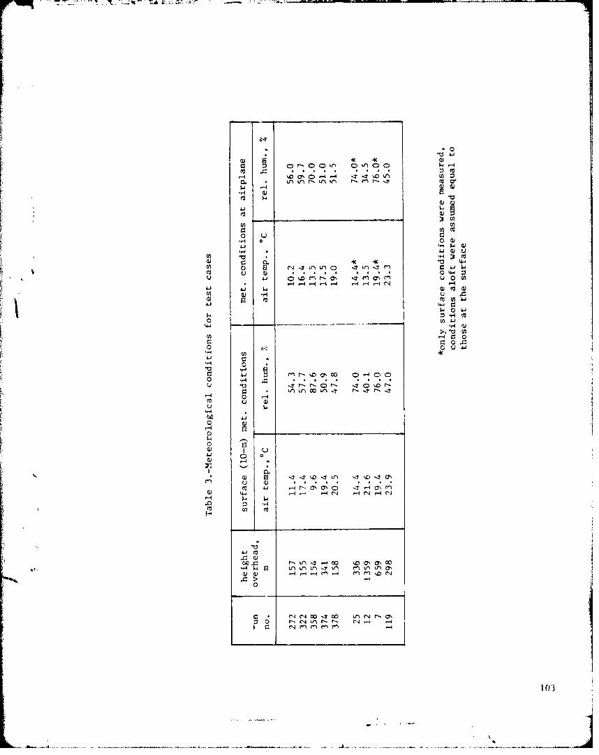
44-
it r lr r- Le) r) r-. r-~
.1 wQ.) U.
"0 4-
U) Aj
U)) CO "4 C
u *ý ý u ;
U) it) .,.4 00 in I .'t
P.4 0- 1-4
1-4
'.44
0 -4
4-j
00
r44 C40 0 n0.4 C' n rf--4 4 ý
rn U) 40r1)-
*10

-0.23 +0.23400
300
200 A
100
E-Ji
-J 0o 8 10 12 14 16 50 55 60 65 70 *-0.6--0 4--0.2 0 0.2zIDo I-,i DCM*14; RUN 272; AIRPLANE HEIGHT, AH, 157 m
040 ___o____ --0,23 +0.23
300I
200I
100 1 6 8 0 5 6 0 6 0 -.- 2 0 : .
0
OCPERCENT dB/100 m
¶ (b) DC-9-14; RUN 322; AIRPLANE HEIGHT, AH, 155 mn.
Figure 24. -Measured vertical profiles of air temperature and relative humidity fortest cases; also profiles of difference between atmospheric absorption
J04
- f '*' 1•••''•''• .• • ,,,'v% '• ,L•",": ,• •• : - - "•• • •,• :, - m .- ,-- - - - -,
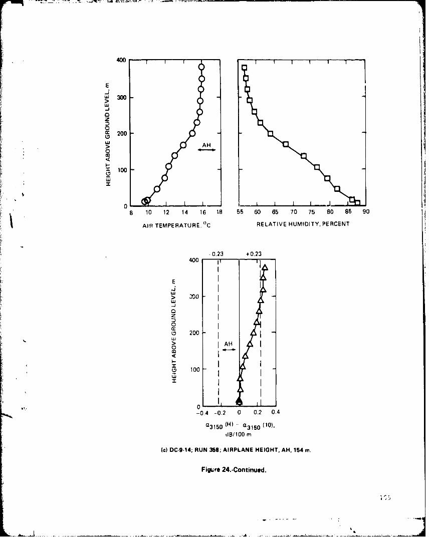
400
E
w 300w
-J
az
0: 200
'U
J> AHO
- 100
0 -
8 10 12 14 16 18 55 60 65 70 75 80 85 90
SAIR TEMPERATURE, (C RELATIVE HUMIDITY, PERCENT
-0.23 +0.23400 -p
E
w
0
-3 I>0 200
'U
> AH
0
-0.4 -0.2 0 0.2 0.4
a3 150 (HI - a3 150 (10),(iBo100
Wc DC-9*14; RUN 358; AIRPLANE HEIGHT, AH, 154 m.
Figu~re 24.-Continued.

400____________-0.23 +0,23400 ;T -I' - -- !
AH
300 -•:200 -
!ES100
-J 16 18 20 22 45 50 55 60 -040. 0 0204
(d) DC-9.14; RUN 374; AIRPLANE HEIGHT, AH, 341
- 0,
>400 -023 +0.23
.00
zI , I
'300 I I;00 --
100 -1 -
016 18 20 22 45 50 55 60 -0.4 -0.2 0 0.2 0.4
AIR TEMPERATURE, RELATIVE HUMIDITY, a,3 150 (H) - a3 15 0 (10),
0C PERCENT dB/100 m
(e) DC.9-14; RUN 378; AIRPLANE HEIGHT, AH, 158 m.
Figure 24.-Continued.
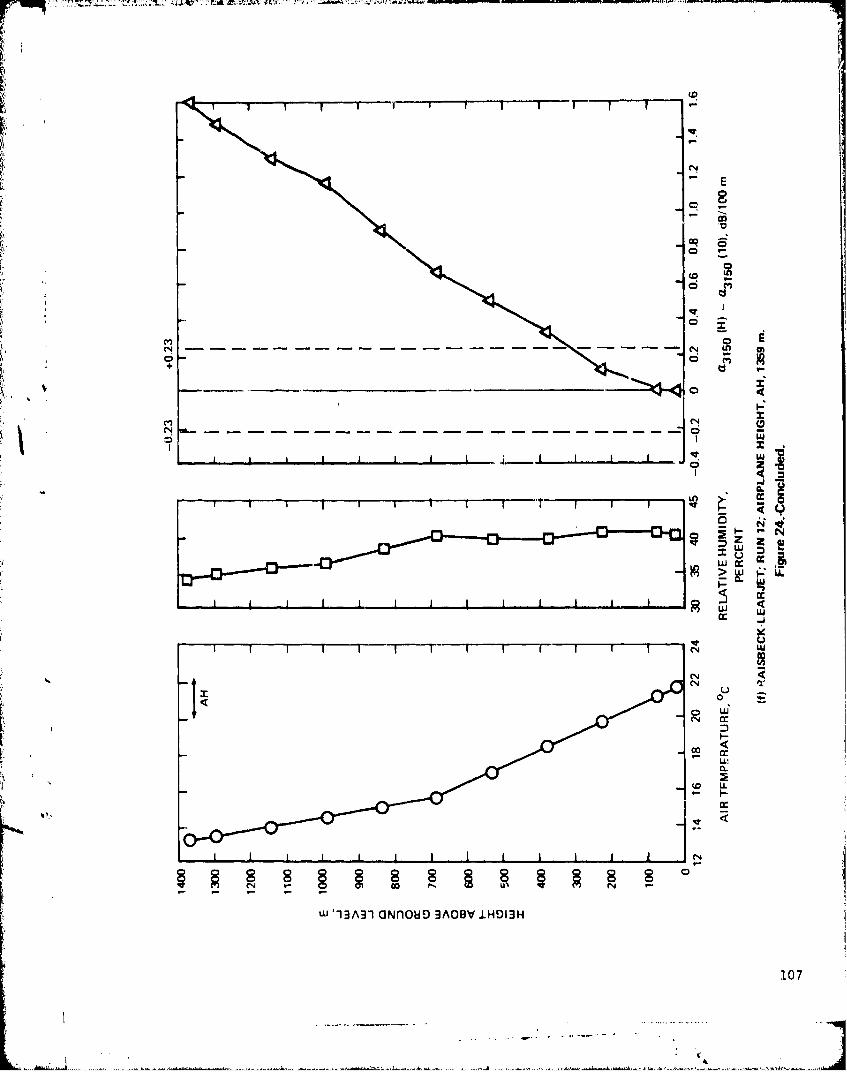
-E
+o
06
U CC
> w ý
-j
N Er 2
co.
SOD N
0107
a midpoint height of about 380 in to illustrate the trends and to extend lhe
profile above the 341--m airplane height of run 374 In Vig. 26(d). In all
cases, the height of the airplane is shown by the double-headed horizontal
arrow in the temperature profile with the label AH for airplane height.
As expla[ned in an earlier part of thi s Section, the FAR '36 criterion forj applying a layered atmosphere analysis in calculating ad justment"; from tes• to• ~reference conditions dep lends onl tihe difference between the at~mospheric absorp-
ttion coefficient (as calculahed ry SoAE AR 866A)i atn a frequtency orf a150 (I,ait a lhe Ight- tip Lo the height of tfie, e2irplane 23 (h1'/ti 0 of sound emission
and tile atmtoslhorie absorption c'oefficient ait 3150 Ilz at tio. surfaCe (1.0,.,
i'i:' , it the lO-in hei, lh ). Tf thils dllftorence exetccds .•()2'3 diB/leO i, Lhen a
layered atmosplhere analysis has to be performed.
The difference in atmospheric absorption coefficients, '%3 1 50(H) - a 3 1 50 (10)
is also plotted for each test run in Fig. 24. It is interesting to note that
none of the five DC " runs that were selected would have required a layered-
atmosphere analysis, even for run 358 In Fig. 2 4 (c) where there was a rela-
LIvely strong temperaturt, inversion In conjunction with a rapid reduction of
relatlve humidity with increasing height. For run 272 in Fig. 24(a), the
atmospheric conditions above a height of 200 in were quite absorptive and data
(If thref, had been any) froum tests at such hi lights would have required a
laye',eti-atLlnosphert, ana lysuis.
"For the Learjet run in Fig. 24(f), the relative humidity was low and did
not decrease by much while the temperature decreased rapidly from the surface
to the lie ight of tLhe aircraft at 1359 in. As a result, the absorption along
the sound propagatLion path was quite a bit greater than at the surface and the
+0.23 d11/l00 m criterion was exceeded at a height of about 300 m. A layered-
atmosphere analvsIs would have been required for the Lear ct data.
A bas ic quantli ty affecth•lg the absorption of acoistic energy by the
' atmuosphere is thi, amount of water vapor present. In the current model of
Satmospheric absorption , the molar concentration of water vapor is used as
the measure of humidity. Molar concentrations were calculated at each height
where meteorological data were available. For each test case, the air pressure
108
. i

at any height was assumed to have the value measured at the 10-m height.
Subroutine MOLAR in Volume 11 was used to perform the calculations.
The resulting vertical profiles of the molar concentration of water
vapor are shown in Fig. 25. Four of the five DC-9 runs [Fig. 25(b)] had
similar profiles with molar concentrations ranging from 1.0 to 1.15 percent
over the range of heights to 380 m. Run 272 [Fig. 25(a)] was different in
t that the atmosphere wais quifte dry (;I molar concentrrat Ion hetween 0.69 and
0. 73 percent) to a lit, iht of abfotit 170 I. Ab)ove thhat ho I 'ht , thit li Id It y
I nr'r(.asctd rap idIly to va Itue orf aboutlt .O 1)(prcent. rhf, mort-humld layer
-I.Iolt aecotints fur tht, lact thaL ithe habsorlpt ion coelfI I Icl nt was lower than
at tHie ,ir fa'ce at he|ights abovo 170 m In FIg. 24(a).
k1 The humidity profile for the Ltcarjet, 11ig. 25(c), was significantly dif-
Sl erent than those for the DC-9 tests. The humidity at all heights up to
1370 in was less than at the surface. The drier conditions at altitude account
for Lhe ahsorption coefficient being greater aloft than at the surface and
for the positive values of the profile of differences in absorption coeffi-
vicvnts In F'ig. 24(r).
T 'ie I, lll1 a.iir colcent raiL Iols i1n I-' Ig. 24 rangl d from 0. 5 to 1.15 pereent wIth
the driest conditions being assý:ocJatel with the August test of the Learjet
,it lr'•sno Alr Terminal. The October tests of the DC-9 (all at Fresno also)
were generally somewhat more humid. All measured humidity values in Fig. 25
were significantly lower than the humidity associated with the FAR 36
conditions for an acoustical reference day. At 250 C, 70-percent relative
humidity, ;ind one standard atmosphere of air pressure, the molar concentra-
t Ion iv 2.18774 percent or two to four times that existing at the time of the
SI yover noise measurements. Thus, in general, it was expected that the
adju:ctment factors from test to reference conditions would be positive, i.e.,
that 00e sound p)res.ure levells would be greater under reference conditions
lthan Under test conditionns, especially at high frequencies.
109
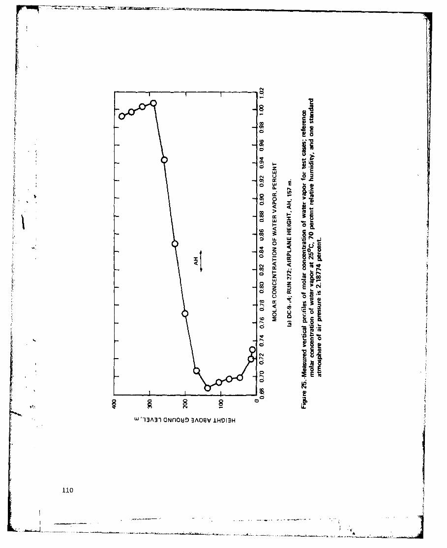
N
Lo
Co
co
0 c
0 .
o0.
40 46 0 cc
CL C
m So
0 m
W'33 ~oD3A1 iH- 13
101U

400
,E 374
L,, 341 m> -,00w
• z0 z RUN NO.
-200HEIGHT0 3 2 2 3 558 737J
a R 155 m 154 m 158 m
I - 10 0 ' 5
I..-
1.00 1.02 1.04 1,06 1.08 1.10 1.12 1.14 1.16
(b) DC.9.14; RUNS 322, 358, 374, AND 378.1400 r ------ T T T
1300 AH
1200
1100
1000E
-Jui 900
.. 800z0 700
"> 600
<. 500•
300
200
100
010.50 0.55 0.60 0.65 0.70 0.75 0.80 0.85 090 0.95 1.00 1,05
MOLAR CONCENTRATION OF WATER VAPOR, PERCENT
(c) RAISBECK.LEARJET; P'-'.ý 12; AIRPLANE HEIGHT, AH, 1359 m.
Figure 25.-Concluded.
111

Sound Propagation Paths
Tn order to calculate the attenuation of sound during propagation through
the atmosphere It is necessary to determine the length of the sound propaga-
t ion path. If tl,e meteorological conditions are not constant over the path,
thet L .'? path must be segmented according to intervals of height over which
average meteorological conditions are known (i.e., by strata or horizontal
layers of the atmosphere).
A description is presented here of the procedure that was developed to
calculate the incremental distances along a sound propagation path. The
procedure is specifically applicable to the geometry of the te- caseA; it
could, however, be readily adapted to other noise-measurement situations.
The symbols and terminology used here are consistent with the corresponding
i!;;ige For the computer program in Volume TI .
We begin by entimerating certain asstimptions relevant to the test cases.
(1) rhe airplane flies at constant speed, Va, and Mach number, M along
the flight path for the duration of the recording of the noise.
(2) The airplane is always at a Large enough distance that the noise
that ir produces can be considered to be emitted from a single equivalent
acoustic source located at the airplane reference point, i.e., the point used
fo," determinin), the location of the airplane on the flight path.
k() ThI flight path is stralgl't for the duration of the noise recording
and Inclin d at an angle, y, to the hotizontal where y is positive for climb-
ing flight and• .,egative for descending flight.
(4) 'Vie sound from the aircraft sourc, propagates at constant speed, c,
alonl!. a straight 1ne to the microphonn, i.e., variations in propagation
oirecticin (refraction) caused by temperature variati, ns (hence sound speed
vnriat.io0s) cnn he negiecLed.
(5) 'The airp a-Le's fl ight path is directly ovr the microphione.
I1!?..*

(6) The height of the airplane, AH, is measured when the airplane is
overhead (i.e., when the airplane reference point is over the microphone).
(7) The microphone is mounted on a stand at a height ZM above the flat
ground plane.
(8) A tiling mark is recorded when the overhead position of the airplane
is measured, i.e., at tfinte TOIl. The timing, mark and the measurements of
height, airspeed, and 'li ght-path angle are the only information available
for tracking the airplane's position as a function of time along the flight
path.
(9) Noise data samples are averaged over 0. 5-s periods and are available
at 0. 5-s intervals throughout tle durat 'on of the noise recording.
(10) The position of the equivalent airplane noise source along the
fIight path Is corrI Ltcd wi Li the t ine at the in id-o int of a corresponding
0. ..- s, si lllf1 c (if n1(1 So' d(t1 l.
It was convenient to ;nalyze the general sIiuation accordlng to a relative
Lest-data-sample t fine, 'IR, dleIf'nc as time relative to the time at the over-
head position.
Time at overhead, TOll, wa!4 provided as part of the input data In seconds
on a 24-hr (86,40(0 s) bas is. The t lie, TS, at the beginning of the first
0.5. s sample of no ise data was also provided in seconds,, on a 24-hr basis.
Thls (TOli - TS) r-'pr.eseits tie time at overhead, in seconds, relative to the
t nin' atL the s'tarL ol Lthel first dlata sample.
"['ihe stream oh 0. I-S no', C dat a sanipLes was des ignated as TT(l) 0.0,
.o(2) = 0.5, TTr(3) = 1.0, T1(4) = 1.5, and so on, where r'r represents test
time and TT(1) is identifled with 0.0 seconds at the beginning of the first
data sample. For the i-th data sample, the test time at the midpoint of the
sample is thus [TT(1) + 0.251 in seconds relative to the beginning of the
first data sample.
113
a11 • J •.• . . . .. . . . . , .... •. , -- ,•- - • • . .. • . . . . •k . .... •.• . ...

T 'lint., III sL ConIs, for the midpoint of anyII data sampljt, rUlat Iw 10 t l111' at
O 1,trh d,;t I! I hum
'IR( ) = '11'(I) + 0.2 To I''l I 'I 'S . (Co )
For any particular sample of daLa (c.g. , the set of 1/3-octavv-band sound
pressure levels associated with the mdximum value of the tone-correctedperceived noise level), the determination of the corresponding sound propagation
path depended on whether the value of TR was ltss than, equal to, or greatex
than zero. that is, on whether the airplane was prior t-, at, or past the over-
head point.
Figure 26 shows the relevant geometrical relationships for the three
I tpossiibilities and df i.nes the important angles 'P and $ and the auxil, lary angle
I).
The airpano files at c~onstant speed V and Mach number M., along the
flight path inclined at angle y. The microphone Is at the receiver position
R near the ground plane.
At ipoint L on the flight path the airplane emits a noise signal which
propa.,at•.., at speed c toward the microphone at sound-emission angle iP relative
to the flight path and the direction of flight. In the time, At, that it takes
for the noise ,Ignal to propagate the distance c(At) trom E to R, the airplane
moves along the flight path a distance V (At) to point P. The airplane positiona
at point P is at angle ' relative to the flight path and the microphone.
The auxiliary angle rn can be readily found from the law of sines for plane
triangles as
c[((At)]/sin(1 - $) = [V (At)]/sin n (53)a
from which we obtain
= a r c s in (M a in ( 5)a (54)
where M = V /c.a a
114
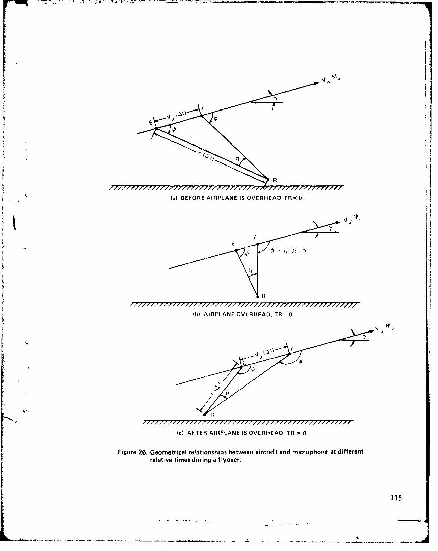
r/i
H11[11//117 77I/1/1 1•IIlll/I~' (.0) BEFORE AIRPLANE IS OVERHEAD,TR<O.
"'•"" ill,-1i111lll/ltlilllllll1111i171111111177ll777=
(h) AIRPLANE OVERHEAD, TR .0.
Ic) AFTER AIRPLANE IS OVERHEAD, TR > 0.
Figure 26.-Geometrical re!ationships between aircraft and microphone at differentrelative times during a flyover.
115

The sound-emission angle, i, which needs to be determined, can be related
to * and n using the trigonmetric rel:Ltion
from which'p ¢ - n(55)
Therefore, if angle q can he found, then angle 'p can be determined using
Eqs. (55) and (54) for a specified aircraft Mach number.
In the special case at overhead when TR = 0, Fig. 29(b), angle € - (R/2) + y.
Note that for level-flight flyovers with y - 0, the sound-emission angle becomes
'p w• ( 1/2) - arcs ln(M ) . arccos(M ) when the airtolane is over the microphone.
'Io d (tLrml ne the values of ,p and ' at times other than overhead requires
the use( of some geometrical relationshilps derived from the available information.
ligure 27 illustrates the definition of quantities used to determine angle € on jthe assumption that. anle y, aircraft Mach number M , and distance from the
mlcrophlw.' to the flight: path at the in, t:lant when the aircraft is overhead are
all known.
Tile calcculation process proceeds as follows:I
(1.) Determinte the distance AMH from the airplane to the microphone at the
t ime of overhead, i . ý. , AMI = Al - ZM.
(2) lFrom AMII and flight path angle y, find the minimum distance U)M to the
f fIig! I path from the microphone at point R (DM - AMH cos y) and tile distance DBi
back along the flight path from the overhead point to the point of the closest
approach (1)B = AMII sin y). 1l1l) ton e IM Is positive' for c'limbing flight paths
when y is positIv( and nt'gativv for descending fl ig ht paths when y is negative.]
(3) 'hl'h. point I' on the flight path is where the airplane is when the sound
emitted at point E reaches the microphone at point R at some specific relative
time TR. The distance D)O along the il ight path from the overhead point to point
11 Is given by I)O = (V )(TR). l)istance DO is negative when TR is negative, Fig.
27(a), and positive when TR is positive, Fig. 27(b).

"• -. AAMH AH
PIAHS
(m) BEFORE AIRPLANE IS OVERHEAD, TR C 0,
!, (b) AFTER AIRPLANE IS OVERHEAD, TR > 0.
4too
•--Figure 27. .Definition of quantities used in calculating angles 4', il, and '4; sound propagation,} distance PD; and aircraft height above the microphone height at the time of
sound emission AHS.
117
r .4

(4) Calculate angle 4, in radians, from
S= arctan(-DM/(DBl + DO)] (56)
whnU 1)B + D)0 ) O, and fromrn
i t = - aretann DM/ ( M + DO)) (57)
Iwhen I) + )0 + 0. When istanMce (IM + D)0) -(0, then poinL 11 Is at the minimum
Ldistance point a1d l - V/2. (Th' nminus sign before DM In the numerator of the
argument of tihe aretangent in Eq. (5•) was included to eliminate negative values
for angle w when ()11 + DO is negatlve.)
(5) Calculate aux1l 1ary angle n, in rad lans, b)y us ing Eq. (54) knowing
M and 4.a
(6) Find angle qj, in rad 1an,, by applying Eq. (55) using the calculated
vaLues of 4 and ii.
(1) l'et ermine tLie total soound propagation pat:h]ength or distance, 111),Irolni
Pl) lk)/s l•l (58)
l0or 11nV relat NOe L i 01Q.
(8) I Inal I y , determine Lhe difference between the height, ZM, of the
microphone and the heipht of the a irplane noise source at loinLt E when it
emitted the sound that reached the microphone at the specified relative time.
lThe height difference, AIIS, is found from
AIS = I') s in(4 - y) (59)
Ior any relative t line.
The incremental d I stanCes , 1(K) , along a sound propagat ion path can now
1W determined '(vcti angles 4) and y and the height difference AHS. Figure 28
illustratev the general scheme for calculating the lengths of the segments of
1.18

E
H (K + 1) 0AHS
HM (K4-I1) -HM MK P..J, K"-; / HM W3)D (K) =
*HM (3)
* HM (2)
o HM (1) ZM
Figure 28. -Illustration of procedure for calculating incremental distances, along soundpropagation path of length PD from R to E, which correspond to heightsHM (K) where meteorological data were measured.
119

-7 -1
the propagation path according tile the heights, HM(K), where meteorological
data were measured. The Index, K, for the array of heights and pathlength
segments starts at 1 for the height or segrinrnt nearest to the ground.
Except for the first and last pathlength segments, the general expression
for calcultat ing tie length of a pathlength segment is
I)(K) = tHM(K+I) -IIM(K)l/sin(i - y) (60) -
for any relative t ime.
"For the flirst pathlength segment, the array of heights is searched to
identify the first hi, ight which is greater than the microphone height ZM.
For example, In Vig. 28 that first height is I-IM(2). The index of the first
meteorolog:ical data height which is greater than the height ZM Is designated
in the computer program by index KK and tile first pathlength distance is
found from
I)(1) [1IM(KK) - ZMI/sin(i - y). (61)
The dilqtance along the last segnent of the propagat ion path (or really
t lt f I rst L c'gtmnit for propagat Ion proceeding from the locat ion of the equ Iva-
t'unt source of noise toward the milc rophone) reqiiIres spec ial consideration
because the height of the airplane at point E will not, in general, coincide
with the height of a meteorological data measurement, The array of meteorolo-
g ical. dta hli ights Is again searched during a calculation to Identify those
he.!1ghtUs (or Indexvs) which I are one auid two less than the height of the airplane
at point. V (incd.xv,, KA and KAI in Fig. 28).
1Index KA Is kused to tern nmite the calculations of D(K) using the standard
f'ormullla in Eq. (60), that is, distance interval !)(KAI) is the next to last in-
terval between the microphone and the .•ource.
'The length of the last pathlength segment Is found from
I)(KA) = (AiHS - IIiM(KA) - /MI I/sin(ip- y) (62)
120

Equations (60), (61), and (62) are applied sequentially to generate the
array of pathlength segment distances over the total propagation distance for
some specified relative test time.
Data Analysis and Adjustment Procedures
The previous parts of this Section have attempted to establish an
understanding abouL the general requirements of FAR 36 relative (a) to
measurement of aircraft noise levels during a noise certification demonstra-
tion test and (b) to adjustment of the measured test-time EPNL to an equivalent
IiPNI, under reference meteorological conditions.
We have also described the characteristics of the Flyover noise data that
were available for analysis. These characteristics Included: (1) the 500-ms
averaging time for each set of 1/3-octave bhad sound pressure levels, (2) the
system used for synchronizing in time the recorded aircraft noise signal and
the position (at overhead) of the aircraft on its flight path, (3) the pro-
cedure used to account for contamination of the signal by high-level background
noise, (4) the geometrical relations available for use in establishing (a) the
angle of sound emission between the flight path and the ray to the microphone
and (b) lengths along the sound propagation path corresponding to the heights
where meteorological data were measured, and (c), for the nine selected test
cases, the nature of the flight paths that were flown and the accompanying
meteorological conditions aloft.
The computer program that was developed to analyze the flyover noise data
From the nine test cases and to calculate atmospheric absorption adjustment
factors was given the name TESTREF for the study of test-to-reference adjust-
ment pcocedures. Volume 11 contains all the statements for the program.
For each test case, the measured 1/3-octave-band sound pressure levels" (corrected for background noise) and the associated test-time meteorological
data, tIme-synchronization data, flight path data, and identification data
were all stored in an input data file.
An analysis begins by reading from the input data file. After reading
identification and flight-path data, the program reads sound pressure level
121
"..'. .•, • , .. .....2 • -.... .. .. ....... ... .. ... . . . . .... . .. ... ... . . .. ............ .. .. ]... .

data denoted by the array SPL(I,J). The index, or subscript, I indicates the
time variable (at 0.5-s intervals) and the index J indicates the frequency-
band-number variable. The .1 index ranges from 1 to 24 for center frequenciesfrom 50 to 10,000 Hz.
For each 0.5-s set of i/3-octave-band levels, the program calculates the
corresponding perceived noise level, PNI(1), using subroutine CPNL, tone-
corrected perceived noise level, PNLT(1), using subroutine P36TC, and A-
frequency-weighted sound level, AL(T), using frequency weighting factors forV 1/3-octave bands from American National Standard S1.4-1971 for Precision Sound
Level Meters.
The sets of PNL(1), PNLT(l), and AL(I) data are then searched to find the
maximum value in each set [i.e., PNLM, PNLTM, and ALM, respectively] and the
relative time of its occurrence. The sets of 1/3-octave-band sound pressure
levels that are associated with the times of PNLTM and ALM are identified.
The sound pressure levels are identified by codes for the two particular times
as SPL(IPTM, J) and SPL(IAM, J) and, for convenience, are given the special
names SPH'TM(J) and SPLAM(,) for the sets of band levels at the relative
test-time indexes IPTM and IAM.
Adjusttment factors for atmospheric absorption losses are calci.ul.ated fortho sotlud villission aungles and propagation pathlengths applicable to the rela-
tive test-time Indexes TPTM and [AM. The adjustment factors are applied to the
test-time measured sound pressure levels SPLPTM(J) and SPLAM(J) to yield
corresponding values for reference-day band levels. The program also reads the
"input file to obtain the measured values of air temperature and relative
humidity at each height and the air pressure at the 10-;n height.
The next step is to cal(Ulate the effective perceived noise level and the
sound exposure level for the ONI.T(T) and AL(.) data, respectively, using Eqs.
(50) and (51). Program subroutine INTE(. Is used to Integrate the data given
the l0-dB-down values, in decibels, of PNLTM - 10.0 and ALM - 10.0. The dura-
tion [actors, I)CF and I)SEL, for the test-time values of EPNL and SEL are found
by application of Eqs. (48) and (49).
122
~ A------------.... .

Reference meteorological conditions are defined for air temperature,
relative humidity, and air pressure.
If t ,eHt-time meteorohlogical data w(,r, 110t il.,a.tir o- at a livighl of 10 m,
then data at 10 m are estimated by interpolnting betwen data menstired at
heights which are less than and greater than 10 m. The second height is
assumed to be always greater than 10 m. The first height where data were
measured is assumed to be < 10 m.
The average temperature and average relative humidity over each layer ofthe atmosphere are then calculated from the measured data interpolated to the
time of the test and read from the input data file. The air pressure measured
at the height of 10 m is assumed to apply to all heights up to the height of
tthe airplane.
'Ilhe final stel) before cal cul.at lug the atmo,,pherl(-,:-aisorpti.on adjustment
factors is to determine, at the relative times corresponding to IPN],TM and
ALM, the total length of the sound propagation path and the lengths of the
segments corresponding to the heights where the meteorological data were
measured. The relative test times at time indexes IPTM and IAM are found using
Eq. (52). Given the flight path angle, the airplane height at overhead, the
airspeed, the airplane Mach number, and the microphone height from the input
data file, the program determines the propagation path distances using Eqs.
(58), (60), (61), and (62). Airplane height at the time of sound emission
I•s found using Eq. (59).
Four alternative procedures for calculating 1/3-octave-band atmospheric-
absorption adjustment factors were included in the study. They were
(1) absorption coefficients and band attenuation by SAE ARP866A
and meteorological data measured only at 10 m;
(2) Absorrition coefficients and band attenuation by SAE ARP866A
and a layered-atmosphere analysis using meteorological data
measured at various heights;
123

(3) absorption coefficients by ANSI S1.26-1978, a band-integration
method to calculate attenuation, and a layered-atmosphere analysis
using meteorological data aloft; and
(4) absorption coefficients by ANSI S1.26-1978, attenuation calculated
at the band center frequenci-s only, and a layered-atmosphereF. analysis using meterological data aloft.
"For each procedure, the set of calculated reference-day band levels isused to determine values for PNL're PNLref and AL't . The reference-day
Nef re ref,effective perceived noise level and sound exposure level are then found by
applying Eq. (46), namely from
EPNL = PNLT' + DFe(63)ref ref test
and
SEL = AL' + DSEL (64)ref "ref test
using the previously calculated values for DCFtest and DSELtest.'
Procedures (1) and (2) are the 10-m and layered-atmosphere procedures of
FAR 36. lI'-oCeudtir (4) is similar to procedure (2) except that absorption
is calculated by the method of ANSI SI.26.-1978 instead of SAE ARP866A and
center frequencir:s are used for all frequency bands instead of just to 4000 Hz
with lower bandedge frequencies for the 5000 to 10,000-Hz bands. Procedure (3)
uses the method of ANSI S1.26-1978 to calculate absorption but evaluates the
adjustment factor by integrating over the bandwidth of a filter.
The methods used for procedures (1), (2), and (4) are relatively straight-
forward. The method used for procedure (3) is more complex because of the re-
quirement to evaluate an integral.
For procedure (1), the reference-day band level for any band is found from
124

SPL ref,()= SPItest + (test, 1m- a ref)(PD) (65)
using the calculated value of total propagation distance PD in meters for
absorption coefficients a in decibels/meter.
The absorption coefficientq a::::: 2a and a ref are determined using a
computer-program subroutine called ARP866A. To find a the sub-test, l10'thm sb
routine is supplied with the air temperature and relative humidity at the 10-m
height for test-time conditions. The 250 C and 70-percent relative humidity
V conditions are supplied to calculate aref.
For procedure (2), the reference-day band levels are found using
Slref,( 2 ) SPLtest + (•test -aref)(PD) (66)
where a is tihe average absorption coefficient under test-time conditionsF. test
over the sound propagation path.
The average absorption coefficient is determined from
=test = atten/PI) (67)
where atten is the total attenuation in decibels over the path. The total
Sattenuation is found from
KL
atten a [te(K)][D(K)] (68)
K=1
where a (K) represents the average atmospheric absorption coefficient by2•.,.test
SAE ARP866A for the K-th segment of the sound propagation path. The index KL
represents tile last segment of the path from the microphone to the airplane.
For each of the K-th segments, the average temperature and relative humidity
for the layer is used with subroutine ARP866A to determine the value of
a test(K).
"125
-

The structure of Eq. (66) was chosen to be parallel to the wording of
FAR 36. Equations (66), (67), and (68) could have been cobrhined as
K11
SPLref,( 2 ) SPLtest +E [a tst(K) - ref][1)(K)] (69)
K=1
since af is a constant and 2I)(K) = P). The method implied by Eq. (69) is
superior to that of Eqs. (66), (67), and (68) from a computational point of
view because the adjustment terms in the summation are all relatively small
numbers and hence the overall accuracy should be better.
For procedure (4), the formalism of Eq. (69) is used to calculate the
reference-day hand levels, namely
KL
SPI,= SPL[ae(K) - a r][D(K)] (70)Pref,(4) test - test rpfK=1
where now the atmospheric absorption coefficients are determined by program
F subroutine ANSAB for American National Standard ABsorption for the test and
reference. meteorological, conditions.
The band-integration method for procedure (3) is described in the next
Section.
Description of Band-Integration Procedure
For procedure (3), the expression for calculating the reference-day sound
pressurL levels is given by
SPL MI~Lý + BA (71)ref,(3) Ltest (3)
126
I"• •. ÷ ... .I

where the hand-adjustment factor, BA( 3 ), in decibels, is determined by a com--
puter-program subroutine called NUMINT for NUMerical INTegration.
The basis for the method of calculating the band-adjustment factor was
derived using an analysis similar to that in Section 2. Tile 1/3-octave-band
filters were assumed to have ideal filter-transmission-response characteristics
because indicated or measured band levels that were not the same as those which
would be indicated by filters having ideal response characteristics were con-
sidered to have, effectively, a measurerent system error. 'Tle "correct" hand
levels were considered to he those which would have been indicated by filters
having ideal response characterristics.
"In making tih assumption about ideaL Ilters, It wa.; rcognized, as a
result of the analysis presented in Section 3, that some of the measured fly-
over noise data may have. contained high-frequency band levels which were
influenced by energy transmitted through the filter's lower stopband. Never-
theless, because there was no way to confirm the suspicion of real-filter
effects for the data that were available and because development of a pro-
cedure to u.ie the response characteristics of real filters with actual aircraft
noise spectra was not within the scope of the present program, the band-integra-
t Ion methcd of procedure (3) was based on the assumption oF ideal filter-response
'haracter 1st Ic,.
Th, assuInpt ion of ideal charactQrisLtics for the 1/3-octave-band filters was
considered to have negligible effect on the valid[ty of the relative evaluation
of the four alternative atmospheric-ahsorption adjustment procedures, especially
for evaluations in terms of time-integrated measures such as EPNL or SEL. Eval-
uation in terms of relative differences in band sound pressure levels, especially
the high-frequency bands, was considered likely to be Influenced more than eval-
tat.ion•s In terms of time-integrated measures by the assumption of ideal filter
transmission response. However, for the data available to the study, the number
of 1/3-octave-band sound pressure level evaluations that could be made was
limited because of contamination by high-level backgi-ound noise in the high-
frequency bands.
The band-adjustment factor for procedure (3) was derived as follows using
127
lj Si 4

, .. 7..............•!-�. -• •,-•.. •, -. _ _
notation introduced in Sections 2 and 3.
'FThe sound pressure level in any band that would have been measured at the
receiver location under reference meteorological conditions (i.e., the bandlevel. Iref) can he obtained from the level measured at the receiver location
under the actual, or test, meteorological conditions, LRtes, by applying an
adjustment factor as
LR re l= + (1R LR (72)ref I'test r f - 'test)
where the hand-level dif'ertRnee - ,R ) ti the adjustment factor BAwhrekt~nu.(1ref test (3)
V In Eq. (/I).
The band-adjustment factor in Eq. (72) can he written in terms of the ratio
of the mean squared sound pressures as
(lR. - Rtest) 10 log [P,re 7R,test]
which can also he expressed in terms of the ratio of the Fourier transforms of
the power spectrum, GR, of tilth Sound pressure at the receiver location as
(Re -lRtest) = 10 log fIf G,ref df /[ U test df (74)L,
[f the filters have ideal response characteristics so that the range of integra-
Lion only need.s to cover the fi. ter's passband.
To evaluate the Integrals in Eq. (74) requires an expression for GR,Cefin terms of measured or known quantities. By analogy to thi development of
EIqs. (17) and (26), the required expression is obtained by writing the spectrum
"at the receiver in terms of the spectrum at the source and an atmospheric-absorp-
tion functi on.
Th Ilius , sVmbol I 'av, the sotind ptresstw ,;pectrtrm at the receiver under the
two meteorological conditions can be written as
128

G(c) (A F )R,test S Ltes
and
(G (AF' (76)R,ref S ret
where AF- is the absorption function over the sound propagation path from the
source to the receiver under the noted atmospheric conditions.
If the sound emission angle I.s constant, then the source pressure spectrum,
GC; in Eq. (75) Is equal to the mource pressure spectrum in Eq. (76). (The
sound propagation pathlengths and the source st.rengths are assumed to be iden-
t Ical under tilte two meteorolo),, I cal cond I t ions. )
I.'rm o I .i (7'I ), the H 0tmtt' i) re iss v spec L rum i s
( G R, tet /AFtest.(77)
R,test te+st
+where the notation Al Indicates the absorption factor along the path from the
receiver to the source, sOe Eq. (26).
With Eq. (77) , the sound pressure spectrum, CG , in Eq. (76) can be
written as
C C )(A-'~ + (AU F ) (78)R,ref R,te.t test ref
Substitution of Eq. (78) into Eq. (74) yields
(IR - I1 t U.;) = BA
10 log )( ts 9 (AU' + (A Ft .fG d (79)(CR, test) tst refR, testd
129

Referring back to Section 2, the form of Eq. (79) is seen to be similar
to that of Eq. (28) with the inclusion of the AF tern. as a factor in the
integral in the numerator.
Because the sound path is to he divided Into segments according to the
layers of tile atmosphere, the absorption function at any frequency has the
form of Eq. (20) namely
+~ k ktest •k,test/10
and
AV/10I'A 20 ak,ref ~k r,r/ef (81)
ref
wholere a [LS the a tino lHlier c sound absorp tion coevfficient appl cable to the k-th
sugment (if the propagaLlon paLh undtr test or reference meteorological conditions
and rk Is the length of the k-th segment. Moltoro logi cal pirnmetors appI Icable
to a path segment are assumed t( be the average temperature, humidity, and pres-
Hure at the mIddIe of each layer of the atmosphere.
Ithe I' oiuiLid path Is dI ivided Into the same segment&; under tiie two atmospheric
condit ios; (as It usual.lv would be) , then rr- r - , and the product ofk,test ~k,ref 'k
the absorpt ion functions In Eqs. (80) and (81) can be written as
- (ak,test - akref) •k/10
(AF +t(AFref) - 1 0 k (82)
and Eq. (79) for the band-adjustment factor becomes
r 1. I (a~ ktest - k~ref) o 1BA(3) 10 log 0 (c, ) IR )df I
(3) ,Jf~ tst ](83
fU (:RCt df
130

Equation (83) defines the band-integration method carried out by subroutine
NLIMINT f'r calcuilat Ion of aid. litiLmunt t'a(tors iv:., procedure (3). Evaluatlun of the
.Intgrals I,4 relatvtI-y ,t5ralghtlorward If an e - x Irc,,fon can he muppi led Ifor the
power spectrum of the sound pressure at the micropho-vu, GRgtest, given the mea-
sured 1/3-octave-band sound prer-sure levels. St.broutine ANSAB is used tc cal-
culatc the values of a and akref by the m.thod of ANSI S1.26-l9)g.
the technique selected to approximate the power spectrum of the sound
V• pressure was the same two-straight-line or two-slope technique used to evaluate
the integrals in Eq. (28), see Figs. 8 and 9. Any iothod of approximating the
a autual shape of the power spectrum of the sound preý-sare at the microphone,
te(f), over the frequency range. of cho pansban,. .-'.f a filter that was moreH, test
sophisticated than the two-straight-line or two-slope method was not felt to be
appropriate. (Sutherland and B~ass discuss the use of a spline function as a
genieral interpolnt ion method between two band-leve, ldat a po ints but recommend
it .log-i linear uvquat Lon to Into rpolate a spoctral shapt, I based on hand leve Is for
tlie hands below, at, and aboV, thi band of nt vrest,) The two-straight-li n,
method was considered to be the best choice becatuse the data were available
only in 1/3-octave-wide frequency bands, because the possible contribution of
energy transmitted through tie lower or ul.,,er stopbands was neglected as a
re, sult of making the assumption that the filters had Ideal response character-
ist~ics•, and because of the necessity to work with practf[cal spectra from which
band levels were missing because of background noise contamination.
Moutegani 2 has developed an aIteornatlve method for numericalty evaluating
the integrals [such as those in Eq. (83)] which express atmospheric absorption
loss over the frequency range of an ideal bandpass filter. As for the present
analysis, Montegani uses band-level differences, or a two-slope technique, to
approximate the power spectrum of the sound pressure at the receiver, GR, but
he defines frequency steps across the range of integration on a logarithmic
"rather than a linear scale as done here for use with the numerical integration
routine available in subroutine QSF. For the i-th frequency band, Montegani
recommends dividing the interval from f, to fr into .1 steps according to
(fr /f ) - lO(3/10b)jj/(2m + 1)1 (84)
131
where bdivlth'te; the type of fractional-octave-band [1 her (h) = 3 for 1/3.-octavc
ball", Eilto s) and Il is an in tege r who.,e( vna1ie I s sp'ci[fi ed by thle user. For all.1
ban11ds, Xo{mtoegan I rocotltlimndn, III: 3 to )-IVe' neven f requene eni ~ioqt ily mpacedl
It Ioi tr j -III t o fil h b tweenl I anld I oii a I loga r ithmtic sca I e
tror I ong -d I-. t on~cv fineaurcuin t L s~ (I' 5011,1, the hIf gi-f frequency port I m) ()I thle
spect runt ('an (Ilecreaso very rapidly' w Ith freqluencY, e,.g. , vec FI g. 4. I)c termi flat I on
o1 L atmosphe r Ic albsorpt I onl I osmen for surh ca8(cM may rep: Ire (.a I CI ]III at on at mnore
than three Frequencies inl each hairf or a frcquenc~y hand Lo ma intaini accuracy.
flowever, for those CcaSCS. the indicated band sound pressure level is most likelyto Ibe con taut [lnated by enlergy t ransmimt td thirough the l owe r 5 topband and theI
approximation of' the power spectrum by the two-slope method will. also be less
accurate. Mon~teganI 'R compu~ter progrant in Ref. 21 could be modified to use m 3
ior somte ra uige or 1low- and midl-f requeney b ands and Inocreas ingl lv arger II values for
tue highelir- frequen1cy banIds. A ntore- fundamen ta I need, however, Is ror a trethod
WhitIch, Ilin a oitipla-tita monlii y V f I 12I Clt 111t111n1r , Ii ible I o t i~t e nI(ati the con tr [hut ion
Lo li, ndI il O IMld141.1idpr.-sur Iov I at,4d y rn -IF ILcref fect.s and then cn
Sut~herland, in Ref. 22, has refined the iteration method described in Ref. 7
and has proposed an analyticil. procedure to estimate what the band sound pressure
Levulis would have beenI If thfe filters had ideal rather than prac ti cal. transmission-
r~esponse cha ra ctIeri st s.
'The met hod use~d here I or calIcu 1 at lg band absorp tion loss made use of thle
sante app roach1 an~ thitt used to derive Eq . (29) . The frequency range over the
panshband of aI flitvtr was qplit Inrto two p)arts, from f 11to the band center fre-qutettcy , ,C and fromt f to ft,. Thle two ternin In thle numerator of Eq. (83)
C ~Ctwhitcih are Ident ical to hone inl Eq. (29) except that they include the absorption
func t I i tis an hown Iiti Eq. (83) instead of Just AF + an in Eq. (29)] are evalua tednunerI caI-i',l ly usingli i."and- lovel di f fe~rences (or s lopes) def ined by E-qs. (30) and
(31). '11w' two denominator termts are evaIluated using EqIs. (32) or (33) as
t approprintace for thev value of' the nslope of the. appLi cabli straight-linto approxima-
tion to CRLs
Subroutine, NUIIiNi carries '(itt tite ralcunLtion of Ohe ad Iuntment factor
according to tuec above-described process for evaluatinog thle Integrals in E~q. (83).
The subrout~lIe requiren spoc if (cat ion of (1) the test-time sound pressure
132

levels that are to be adjusted to referen't conditions, (2) the refer-
ence air temperature, (3) the ret erenee relat iv humid I ty, (4) thLe re 'erence
air l)resm, r(, (5) the array of avrage tst-tlne air teinperaturos over each
Inver oi the atmophire start lng at the lie IghL or the mnIcrophoov, (6) t h
Correslmond Ing array or average t vt-t ime rel at ie 1 hum id It I Cs over each iftumoS-
pheric layer, (7) the test-time air pressure, (8) the array of pathlength
segments between the microphone and the aircraft at the time associated with
the sound pressure levels, and (9) the value of the final index along the ''
path from the microphone to the aircraft for the arrays of air temperature,
relatlve humidity, and pathlength segments.
Tue total number of rrequency intervals (or number of frequency steps) *Ivr thie pa4sbannd of n filter that were uted to evaluatLe tiLe numerator terms
VFor Eq. (83) were the same as used with subroutinme QSF In Seet'Ion 2 for thie
Ileven hinuis with center Irehquencles frrom I00) to 10,000 Ik',. Thum, for oxample
the hand at 10,000 liz was dIvided Into 30 equally-spaced Qvteps, 1.5 from f to
f and 1ig from fC to fu. The 13 hands from 'AO to 800 HIz were each dividedC ( U
into 8 steps, 4 From r to r and 4 from r to fU. Four steps is the minimum
numb•r recommended for use witlh the QSF Integoration rout ne.
Civen tihe test-time sound pressure leveln, meteorological and pathlength
dnta, and the nummimbe r 0f rrequvmncy intervals to use for the numerical integra-
Li lons, t.Ltm process of calculating tihe hand-ad usntmentI f actor is strai•ghtforward
With oie texception. The exception is the calculation of the slopes of the
mtraight gine approximations to (GR,tVst over the frequency range of each
f liter.
Calneulation of band-level differences or slopes was not as straightforward
am in Section 2 because of the need to he able to handle spectra from which
band levels were missing because of background noise contamination. The
various possibilities for spectra having missing band levels are shown in
Fig. 29. Subroutine l)IFFS, which is called by subroutine NUMINT, was pre-
pared to handle all the poss ibilitiest and to calculate appropriate band slopes
for any test-time spectrum.
Figure 29(a) illustrates the case when a complete spectrum with no missing
band levels Is available. Slopes (or band-level differences) are computed for
... ........ ..... ,

SLOPE (1,2) .) L.1
SLOPE(,I) SI.OPE(II2)eQg
SPL, dB SLOPE (J, I) SLOPE (J 12)SLOPE (J,2) -Lj+ - Lj
000 I L eeSLOPE (23,2)-- L2 4 - L2 3
1 2 3 **e 101112 13 e 21 222324 SLOPE (24,1) - SLOPE (23,2)SLOPE (24,2) - SLOPE (24,1)
BAND NUMBER
(a) CASE 1: DATA AVAILABLE FOR ALL BANDS.
SLOPE (1,1) - SLOPE (1,2) - SS (1)
SLOPE (2,1) - SLOPE (2,2) - 1,0I SPL, dB • ' SLOPE (3,2) - L4 - L3SLOPE (3,1) = SLOPE (3,2)
AND SO ON TO BAND 24
1 2 3 4 6 6BAND NUMBER
(b) CASE 2: NO DATA FOR BAND NUMBER 2;
ISOLATED BAND AT BAND NUMBER 1.
see FROM BAND 1
SLOPE (21,2) -L 22 - L21SLOPE (22,1) " SLOPE (21,2)
SPL, d8 SLOPE (22,2) = SLOPE (22,1)
IIISLOPE (23,1) SLOPE (23,2) - 1.0re- SLOPE (24.1) - SLOPE (24,2) - SS (24)
- 21 22 23 24
BAND NUMBER
(a) CASE 3: NO DATA FOR BAND NUMBER 23;
ISOLATED BAND AT BAND NUMBER 24.
oe. FROM BAND 1
SLOPE (J-2,1) - SLOPE (J-3,2)SLOPE (J-2,2) - SLOPE (J-2,1)SLOPE (J-1,2) SLOPE (J-1,2) - 1.0
SPL I dB" SLOPE (J,1) -SLOPE (J,2) -+SS(J)
SLOPE (J+1,1) - SLOPE (J+1,2) - 10
""00oSLOPE (J+2,2) - L -+3
1 2 "" , "" 23 24 SLOPE (J+2.1) - SLOPE (J+2,2)"AND SO ON TO BAND 24
BAND NUMBER
(dl CASE 4: DATA FOR BAND AT J, BUT NO DATAFOR BANDS AT J-1 OR J+1; ISOLATED BANDAT BAND NUMBER J.
Figure 29..lllustration of rules for calculating band.level differences.
134
- -..... .. . - - " "'
- : - 7
the lower half and the upper half of each band, see Fig. 9. For a band at
If0,'quIenev-InIti .I, Jhe s lopes ovwr t:hiv lower and upper halwys of tihe, passband
art, tit'I tiot cd by v LIt two-d Illne s I ol ,aI itrrays i 1.0111,:(.l , I) ind SIOPI(,l ,2) , r,,pe't-
Iv'l y.
I'lgure 29(n) also Indicates the rules used I'or computing the s lopc,- for
any of the 24 bands. Note that a special rule was required for thme lower
half of band 1 and the upper half of band 24. The slope over the lower half
of band 1 [SLOPE(l,l)] was assumed to equal that over the upper half of band
1 [i.e., SLOPE(l,l) = SLOPE(],2) - LI]. The slope over the upper half
of band 24 was assumed to equal the slope over the lower half of band 24, i.e.,
SI,0PE(24,2) - SLOPE(24,1) = LP- r Montegani 21 made the same assumptions
for his computer program.
SFl,,turL'5 29(h) to 29(d) IIIIusIratt, the tLlret, spictlal cascs taot nec'dold to
he c'onhldered as i rescliIt of hand Ieve Ls mils1ng from aI ,p)ectrom h 'ltiise ofbackground noise contamination. The three special caases Involve thtl question
of how to specify a set of slopes for a hand that is Isolated in the sense
of not having valid sound pressure levels In the bands above and below. the
three cases also involve the question of what to specify for slopes for the
band for which the sound pressure level is missing because of contamination.
The peneral rules adopted for the isolated-band and missing-band problems
were (I) that the slopes to use for isolated bands were the substitute slopes
shown in Fig. 30, and (2) that a slope of +1.0 dB/band should be used for
bands having no valid sound pressure levels.
The band-level slope of +1.0 dB/band was chosen as a convenient, though
arlItrary, value to use with tie numerical integrations performed by sub-
routine NUMINT. A slope of +1.0 dB/band represents a white-nolse spectrum
with Uqual energy per unit frequency. By Eq. (30), tihe power spectrum of a
white-noise signal Is a constant (i.e., 91 . R, 0).
When the band-lcvel slopes are +1.0 dfl/band, the hand-adjustment factorfrom E~q. (83) represents the difference in the average attenuation resultingfrom atmospheric absorption over the frequen.v range of the pasaband of the
135
.I

21
w -OOO
SO-2- BAND SLOPE, 0, NUMBER dB/BAND
8 20
1 0z .4 1 T03 41 0•. • •. .5 4 TO 16 O"
6 17
15 AN24is AT1 200hI
:" ' • "; 7 -19' 3•" I 204
621{ -" 10 - 22 .. 70 "11 23 .lO0
f:-13
" 14 - BAND 1 IS AT 50He'•15 - BAND 24 IS AT 10,000 Ht
50 80 125 200 315 500 800 1260 2000 3150 '000 800063 100 160 250 400 630 1000 1600 2500 4000 6300 10,000
1/3OCTAVE BAND CENTER FREQUENCY, Ht
Figure 30.-Substitute slopes for 1/3.octave'band levels of broadband aircraftnoise in the free field. (Substitute slope for band 1 estimated fromslope derived for band 2,)
136

ideal filter and over the length of the sound propagation path. For a white-
noise spectrum, Eq. (P3) reduces to
~ rf~ /(ak~~ -ak~ref)Yki0I
BA 10 log I 1 10 ~es ' dfII (f f (85)(3) If i d
where the denominator (fU - f 1) represents the bandwidth of the ideal filter.
Although subroutine D IPPS does supply subroutine NUMTNT with slope values
Ifor the, lower and upper halves of' all 24 bands IncI.tidin g toste hands ,HL I. have
lno v.LId data bhcause of background no0ise contatn U1nt Ion f i and 1101oliglh I Ihrout
NUM TNT does calculate a band-adjustment factor for every hand from band 1 to
hand 24 regardless of the value of the test-time sotind pressure level., the
main computer program is instructed to set the reference-day band sound pres-
sure level to 0.0 dB If the test-time band sound pressure level was not valid.
Thlt is
Sil,r (.1) 0.0, if SP te (.J) - 0.0 (86)rof test
for any biind and for any band-ad ustment method.
'The rule expressed by Eq. (86) was adopted to avoid creatIng values for
retFerence-day hand hiound pre'ssurt, 1 Ve is whtu thv, test-L Iime sound prossture
Iewv l was nl H s InH ,g Blcause, 0l Eq. ( 8), any conveni ent slope cot id Iave been
sel.t e'ed to lisse for SLOPE (.1,,I,[) and Sh (11,(2) when the hand sound preossure
level was missing. The value of +1.0 dB/band was selected I,,tcalv it
yields a measure of the average adjustment factor. The average adjustment
factor was considered to have intrinsic interest. All adjustment factorsare available internally within the program and could be listed in the output,
If desired, with minor changes to the program statements.
'The problem of specirying reasonable values to use for hand-level slopes
Iln the case of an Isolated hand sound pressure level [cases 2, 3, and 4 in
Figs. 29(b) to 29(d)] was resolved by developing the set of so-called sub-
stltute slopes shown In Fig. 30.
137
I " ]

T e sI )I)L'-;hin I'g. 30) re~preSentL 'lv(,r;1), Va 1C 01L1 Iie o ld i d f' iOnl VNI1inI l:ilt It'll
of 1),indi-lev'c . s loipes from 1./3-oct ave-hand spec tra aLI vat. Ioulý t m's- dIirinrlg t ht
record ings of flC-9 flyover noist! levels front the five samples of' test data.
In the low-frequency hands (center frequencies from 63 to 630 Hz), large vanl-
ations in slope (±ý8 to ±10 dB/band) were observed. Thle. large vairiations were
attribuited to ground-reflection effects in the measured spectra. An average
slope of zero dB/band was estimated to be approprnl'e for the broadband
comp~onent of the spectrum in nn acoustic free field. For the high-frequiency
hands (1250 to 5000 lHz), votriations -in observed slope values, were somewhat
smale thn hos osev.ýd for the low-frequency hands and] were nttribued
to discrete-frequevncy components in the YN81 engine noise inl
Tllie Iii gl- I reqtiinvy ro 1101.1. u F the spec trum Impliled hy the( I ncrons I iii'y
negat ive' slopes F'or the bands. above 1600 liz Itt Fig. 'J0 was regarded as being
representativye of* the broadband component of the let-no ise spectrum for the
moderately absorptilye atmospheric conditions andi moderate pathlengths appli-
cable to the available aircraft noise data.
Alternat ives to the. use of the substitute slopes In Fig. 30 for specify-
Ing hand-level sloipes to use with subroutine NUMINT to calculate an absorption
adjustment factor for an "Isolated" band were also considered. The alternativesI
were elthc'r to specify some arbitrnry slope that was the same for all bands
that mighit have Isola~tedl values of sound pressure l evel or to calcuilate. a
Sl~ope based ou the n'art'sL val Id souind pressure leve(ls in bands above at, helIowOlhe hand couILa Inii g the '' 0 ie' )111sound pressure IlovelI. S pee if en tion
of an arb itrary slope (such as +1.0( dIi/band) would have been somewhat ens icr
to incorporate In the computer program than the use of substitute slopes;
the substitute slopes, however, were regarded as being more realistic in the
high-frequency bands. Calculations of slopes, by extrapolating ov~~r one, two,or more bands hayving missing sound pressure levels would have. been more comn-
p1 iCatc(ad would not have been anyv more accurate or appropriate than the
teclun Ique of us ing ai set of stibst ittute slopes.
The slope over the upper half of the band prior to a band where the data
were missing [e.g., the band at .1-2 in Fig. 29(d)] was calculated as though
138

0i!':iI ,the band was the last In a completc spect rmin [I . e, band 24 In Fig. 29(a) ISimilarly, the slope over the lower half of the band above a band where the
V data were missing [e.g., the band at .7+2 in Fig. 29(d)] was calculated as
though the band was the first one in a complete spectrum [i.e., band 1 ina[" Fig. 29(a)].
As a final observation on the band-Integration procedure for determining
the attenuation caused by atmospheric absorption, it is important to note
that the power spectrum of thu ;ound pressure at the microphone (i.e., GR'test)
has always implicitly been assumed to be a relatively smooth and continuuus
Function of frequency. This assumptlon was the basic JusttIfleation for the
"rvastlahbleniss of" ipproximt Inglg C In Eq. (8)) 1 nilt' sgmients, overRI, Levst
the lower and upper hal] ve of the theoretical pasl•4lil of the I/1-o taiv-h•nd
F iters. If' the spectrum oF the sound contains dIscrtc-FrI'requoncy components
" .; such that the sound pressure level In a band is controlled by the level of
one, or a few, spectral components within the paasband of the filter, then
-I the two-slope or band-level-difference method for approximating G as aR,test
I> function of frequency will not provide a reasonable estimate of the actual
variatiton of C with frequency.Ritest
Tf discrete-frequency components are present in the passband of a filter
and If a procedure were available to determine their level and frequency, then
tl 1,Integrati:on of Eq. (83), or the summation carrIed out by the numerical
IIVtc',rat I procedure In suibrott iIii' NIIMINT, wo ild ounIv need to Inclit' l ih' lhe
d I•s,| reut e- I r'i(titntcy comlpolintlsn . I I there Is only (lni' d sI er t, -'r q(liincy cdlm-
ponentl withlin the passband and Its leveI dot rmInL's the lIndicated hand Leve L,
then the integration would include only one spectral component and, for that
"band, the calculation of the adjustment factor would be reduced to the form of
Eq. (70) for procedure (4) but evaluated at the frequency of the component
Instead of the band center frequency.
"In order to lie able to apply the integration method of Eq. (83) separately
to the broadband, continuous component of a spectrum and to the discrete-fre-
quency components, some procedure must be available to provide an estimate of
the level and frequency distribution of the component.-. The procedure 'iould
have an analytical base so that It can he dserhc'bed mathematically and Ineor-
I T9
-------- -.

porated into routine data processing by a digital computer. The procedure
should be capable of accounting for band-sharing effects caused by strong
discrete-frequency components or by moderate-amplitude componencs whose fre-
•i quency Is near the edge of the passiatid of a filter. The procedure shotild
an ;o he ;ble to account for tlit pparient hlang,,, In frequiency di,. to IDoppler
elf l cL, F s L it, magn I lode and s Ign of hith- Coml1OnLo t of the sp'eed of t lie ,sokind
C ssourcues on Lite a ircraft in the dir-eclion of the sound ray p'ropaga t Inip, toward
ithe microphone (and consequentlv thie apparent wavelength and hence frequency)
change with time during a flyover.
A procedure to determine the separate components of a complex time-varying
sound such as aircraft noise does not exist. The nearest approximation to
such a procedure is the tone-identification routine in Appendix B of Part 36
but that method only provides a crude estimate of the broadband, continuous
component and no information on the true frequency and level of the discrete-
frequency components. No analytical procedtore is ava1iable to account for band-
sharing or IlollI r-[rcqule 'y-' ll lf , t:F. Thus, e tither bec'.1se' in1forma7;|tioll Is not
IVawlabIt or cannot Ibe provhilid In a practical maniner, appl i cation of the band-
hintegrol ion method f EqI. (81) wil tzsa |- lliy bh accompl Isised in a :;Lr;li,,ItL-forward man ner i)V ignor Ing aniy ,sos pe t'cd or atr u cLual dis('rctc-[requency com. p('nunts
and simply estimating the pressure spectrum function G by the band-levelV 'R,testdifference method across The passband of every filter.'I,,
The straightforward approach was adopted for this study when using the
',hand .integration method of procedure (3). The band-level adjustment factor
determined by such an approach will be incorrect although the error, as
Montegani 2 ' has pointed out, will potentially be no larger than using tihe band-
center.-frequency method of procedure (4) and ignoring the integral approach.
Results of Comparative Evaluations of AlternativeAtmospheric-Absorption Adjustment Procedures
.Previons parts of this Section have described the nine cascs of flyover
noise data that were available for analysis. The description included consi-
- deration of the procedures used for acquisition and processing of the flyover
noise data as well as consideration of the available tert-time meteorological.
, data. The method of calculating the lengths of the sound propagation paths
140
!A
and the angles of sound emission at times during a flyover was shown for the
geometry of the test cases. Also described was the computer program, TESTREF,
that was prepared to analyze flyover-noise test data and to determine the
sound pressure levels that would have been measured under specified
reference-day meteorological condltions instead of the :ic t e st-timemeteorological conditions. Four alý:ernatiw, proeedtiros were conside.red f or
calculating the band-Level adjustment factors for diiference s In atmosphericeabsorption under test and reference conditions. l',valoat lon of those four Iprocedures is presented In this part.
Evaluation of the atmospheric-absorption adjustment procedures is given 'j.
here primarily in terms of the effect on the 1/3-octave-band sound-pressure- r
level spectra. Evaluation also includes a discussion of the effect of using
the various procedures on the following noise descriptors: PNDI, PNLTM, EPNI.,
ALM, and SEL
S4( aau?'oc/ / Z'Y' I ', i c'c" / N,,'j;- I, / tfl,/ A- atqh, tot ,U'OLd Icveh "[,.- We begin by
considering the variation of PNIT and AT, wih tLime Jur ing a typIcal flyover
no 1ise imeaisureimient. IFIgulre '31 presvents the results at 0.%-s t line mrt rva ik
relat. i•;tL to the t lin1e when| the airldane was ovwr the miic'roplione, i.o.. tife
'I' (I) by Eq. (02). The I'NIT and AI, vaties were normalized by t heir respe(,tiv(y
maximum ievels, PNLTM and AIM. The data are from run 272 of the set of 1)0-9-14
tests, see Table 2. The subcaptions for the two sets of data in Fig. 31 list
the values of the maximum quantities (PNLM, PNLTM, and ALM) as well as the time-
integrated quantities (EPNL and SEL).
The plots, in Fig.. 31 illustrate some features that are significant to a
study of atmospheric-absorption adjustments. The primary scale for the abscissa
is the linear scale for the time TR(T) at the midpoint of a data sample relative
to the time at overhead. A secondary abscissa scale is shown below the time
scale for the sound emission angle p. Note the rapid variatiun in the value of
""i around the overhead position. In the two-second interval from TR= -1 s Lo TR
= +ls, 0 varied from 53.20 to 1.02.30 or about 250 per second. The rapid varl-
ation In angle emphias izes the need for having a hlhli-quality airplane-trackingI
system during a test and for having, accurate synchron[zation in time between
the airplane tracking system and the noise recordings.
141
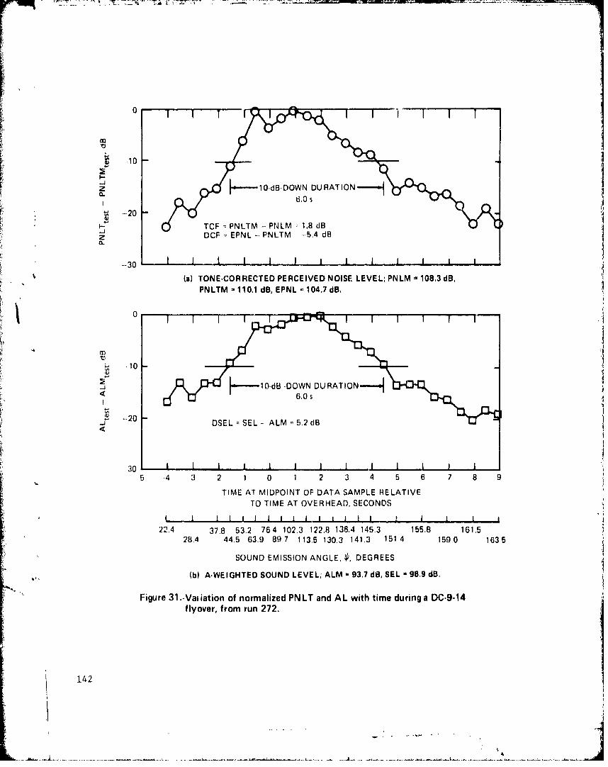
0,
-JI- -10
Z ý-10-dB-DOWN DURATION-.0.O
-20
I- TCF ý PNLTM - PNLM - 1.8 dBZ DCF EPNL PNLTM -5.4 dB0.
--30 ., I I , I , I ,1 ,
(a) TONE.CORRECTED PERCEIVED NOISE LEVEL; PNLM 108.3 dB,PNLTM I 110.1 dB, EPNL = 104.7 dB.
0
.10
30 I I I I I I
5 .4 3 2 1 0 1 2 3 4 5 6 7 8 9
TIME AT MIDPOINT OF DATA SAMPLE RELATIVETO TIME AT OVERHEAD, SECONDS
30 I 1 i ! I 11 1 1 1 1 l I 1 I 1
22.4 37.8 53.2 764 102.3 122.8 136.4 145.3 155.8 161.528.4 44.5 63.9 89.7 113.5 130.3 141.3 1514 159.0 1635
SOUND EMISSION ANGLE, b, DEGREES
(b) A-WEIGHTED SOUND LEVEL; ALM 93.7 dB, SEL 98.9 dB.
Figure 31.-Vaijation of normalized PNLT and AL with time during a DC.9.14flyover, from run 272.
142
-./. .

Another point is that, although the time variation of VNLT and AL in
Fig. 31 Is relatively smooth, the time pattern can contain several .bhrrt-
duration peaks. Indeed, for the PNIT data In Fig. ll ,I' the peo.i -It thbe
relative time of -0.55 s has a valetu whiclh Is only 0.1 dBi below tih maxilmiin
"at +0.95 s. if tile peak at -0.Y) s had been 0.1 dti hightur and thi peak at
0.95 s had h,.,en 0.1 i dl lower, then thi sot(nd emis.4inn angle associated with
PNLTM would have shifted from 102.3' to 63.90 with a correspondingly large
change Ln the length of the sound propagation path and the magnitude of the
calculated band-level attenuation due to atmospheric absorption.
Note ralso that if there had been two or more peaks having the same
maximum values, the one chosen to he destgrlated as PNLTMI (and its corre-
sponding time or emission angle) is always the last one in a search from the
first. to the last data sample. The choice of which maximum to designate as
i PNL'I'N or ALM does not affiect the dettrminination of tht, 11-dii-down integration
tLimus or the value of the 00ltegrated measures E11PN, or Sli,. 'I'lh! cholot of the
Hjim, of occurrence of i'NITMi or AIM do•s, howev.,r, ali' vttth, .1 en)gth of Hth sound
propi'-galt Lon pat!i and the caicouLaLion of the hand- :veIL tidjust:inent f'actorn from
Lest to reference meteorological cond it ions,
In five out of the nine test cases, the time of occurrence of PNLTM was
the same as the time of occurrence of ALM. Figure 31, however, shows one of
the coses where thu re1 at. V imoP.q were not the same. The maximum sound
lev(,l ,c.curred at +L.95 s, a't an angle of 122.8' or one second later than
'NIT'M at an angle of 102.:. 3 Depending on the spectrum of the sound signal,
the time of ALM could precede or follow the time of PNI,111, although in three
of the four cases where the times were not equal, the time of AiM occurred
iafter the time of PNLTM by 0.5 to 1.0 secondsi.
'lThe Lone-correction factor (TCF) of 1.8 dil shown In Fig. 31(a) was th(e
largest value obtained for the nine Lest cases alt bougih a value of 1.8 dB was
also obtained for run 358 as indicated below,
143
<4
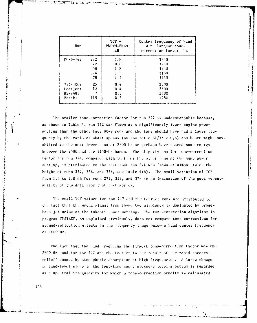
TCF Center frequency of handRun PNLTM-PNLM, with largest tone-
Ldil correctlon l'aetor, INl
)IC-9--14 : 272 I.8 '11 'i()
SI: IIi('122 0.6 11W'374 1 .3I 3i110
'..378 1. 5 31 SO
727-100: 25 0.4 2500Learjet: 12 0.4 2500HIS-748: 7 0.5 1600Beech: 119 0.3 1250 i
rhe smaller tone-correction factor for run 322 is understandable because,
as shown in Table 4, run 322 was flown at a significantly lower engine power
settlng than the other four I)C-9 runs and the tone should have had a lower fre-
-Itoeney hy the ratio of s.halft Hpeeds (1y the ratio 61/75 v 0.8) and heiv(..e tl hli : hav
'it I I.It ed to Ihe next lower bantl at 2 ')00 II z or perhapH havie "itrruid ,ome onrfy
tOu'twOV II th 2'u() 11l11 the Il'()-Il',, MiddO.W 'liii si , ghI ly tnmnlllor toyio-corri-,t Ioli
I actor fot ron 1/4, compared with that lot, the ot her runs a; t t hi e :tho !tt., piwvir
,tvtti.ng, t1 aitt rlbutLd to thhe Fact thant run 374 was l'lown at almost twice the
height of runs 272, 358, and 378, see Table 4(b). The small variation of TCF
from 1.5 to 1.8 dLl for runs 272, 358, and 378 is an indication of the good repeat-
abhi. ty ef the data from that tet series,
The Sm11 '[1 TCl" vallue S for the 727 and the lxearj et runs are lttributed to
Sthe fact that the sound signal from those' two airplanes is dominated by broad-
"band jet noise at the takeoff power setting. The tone-correction algorithm in
program 'I'I'STREF, as explained lpreviously, does not compute tone corrections for
ground-refLection effects In the frequency range below a band center frequency
of 1000 Hz.
The fact that, the hbandi produc li, Ilie lrirg.est tone-correct fon iactor wns the
2500-liz hand for the 727 and the lezar et Is the result of the rapid spectral.
rollolf c ius d by ttmospheric absorption at high frequoncies,. A large change
in band-level slope in the tcst-time sound pressure level. spectrum is regarded
as a spectral irregularity for which a tone-correction penalty is calculated
144
k • . "... .... • . . .. . . . . . ," ,

Table 4.-Engine/airplane parametersfor I)C-9 runs
(a) engine parameters
nominal engine engine enginerun thrust pressure exhaust gas LP shaftno. per engine, ratio temperature, 0C speed, pct
kN left right left right left right
272 26.7 1.44 1.44 370 375 75.1 75.0322 13.3 1.205 1.205 322 321 61.2 60.9358 26.7 1.44 1.44 380 380 75.9 75.2374 26.7 1.44 1.44 390 380 76.0 75.5,378 26.7 1 .44 1.44 J90 385 70.11 75.8
(b) airplane parameters
airplane airplane flap nominal nominalrun gross weight height deflect, airspeed, flight'no. at overhead, over mic, deg m/s Mach no.
kN m
272 344.9 155.8 33 71.7 0.213322 312.2 153.8 0 78.3 0.229
358 334.3 152.8 38 74.4 0.219374 315.8 339.8 38 73.5 0.215378 302.1 156.8 36 72.6 0.212
even thou.gh no discrete-frequency is present.
For tih two proupellr-powerd airplanes, the spectral. irregularities rt Ia, Ld
to the fundamental and harmonics of the blade-passing frequency in the bands
at 100, 200, and 400 Hz were ignored in calculating tone corrections.
Spectral irregularities for center frequencies above 1000 1iz were caused by
atmospheric ahborption and yLelded the 0.5 and 0.3-dB tont-correction factors
shown In t he table on page 144.
To eomplet,, the discussion of the results in Fig. 31, consider the duration
factors DCI for IININ and DSEI, for S,'L. It is interesting to note that DSEL can
"be closely approximated by the quant ity (DCF + 10). To see why this should be,
"and to derive a useful relation, we re-write Eqs. (50) and (51.) by introducing
145

the maximum values J'NLTM and ALM. The working definitions for EPNL and SEL
can then be re-cast into the format of Eqs. (48) and (49) where the duration
I(.acltors are givwn by
DCI' L) log, . I (PNI.T(I) - INI,'I'M) + 1( log (At/lE) (87)
and
t 2
DSEL 10 log 1 0,l(AL(i) - ALM] + 10 log (At/to). (88)
If, as suggested by the two plots In Figs. 31 (a) and 3 L (b) , the time varn-
a:Ition of' the norll, Ii ized quant lties [IPNIT(1) - PNLThM] and [AL (I) - ALM) is anpprox-
Imatl, ly the same over the plri lod of Ll me betl.ween Hit, l0-dif-down tIlim., I' and 12,
I.h1,i the two duration correcLion 'ictors sh ,oil1d only differ by 11) tlm: ,,m l.he,
Ilega i itlh1l (l1 Lie, ratito of thu rel'erenc , t imes iI.:/I
Thus,, Ohe fol lowing approximat lu01 hold hold:
DSEL DCO + 10 log ( /Lt ) (89)
or
I)SEL DCF + 10. (9o)
The'lu reference times of t 1, =0.0 s and to 1.0 s were used to obtain Eq. (90).
Equation (90) could be useful in a situation where the EPNL and the duration
factoi DCF were known and ALM was also known and it was desired to obtain an
estimate of SEL for the same recording of flyover noise.
Another uselut r, 1lati oiu hL' Lwe('nii the dural1 on f (ac'tors can be obtained by
approximately Lhl, Lhape o0" the time variat fon of I'NI,T or Al, between the l0-dB-
down times by i triangle with a base qoual to the 1O-dB-down duration time
1.46

(tD, or tDA or simply tD). The vertex of the triangle is at 0.0 dB for the
normalized quantities at the time of PNIIH or ALM.
The height of tile triangle Is given by the difference between the power
ratios at 0.0 dB and at 10.0 dB, i.e., by the difference between 1.0 and 0.1
or a height of 0.9 in terms of power ratios for the normalized ordinate scale.
The area of the triangle approximates the area under the plot of [IPNLIT(i)
ri - P'NLTMI] or or (AL(i) - ALM] In Figs. 31(a) and 31(b) and, effectively, prov ides
an alternative way or evaluating IEqs. (87) and (88).
Thus, Cor the normalized PNIT plot we obtain
* DCV 10 log ([(1/2)(t )(0.9)]/t }
10 log tDF + 10 log (0,9/2t j) (91)
10 log t - 13.51t), E
and for the normalized AL plot we obtain
DS Eh 10 Log L[(1/2)(tl),A)(().9) (/t (92)
10 log tIA - 3.5.
1)
We can use the value of 6.0 seconds shown in Figs. 31(a) and 31(b) fort D,E and tD,A to test the validity of the approximations in Eqs. (91) and (92)
rThus, for run 272, Eq. (91) gives -5.7 dB against the calculated value of -5.4 dB,
while Eq. (92) gives +4.3 dB against the calculated value of +5.2 dB. Additional
comparlsons are given in Table 5 for the approximations given by Eqs. (90), (91),,nd (92) wi th durat I o- factor va 1 nes caI cu ated from Eqs. (50) and (51) using
com)utiLr-program subroutine INTEIC. The approximate duration correction factors
are within one decibel of the values obtained from the measured data.
The data shown in Fig. 31 were typical of the time variation of airplane
noise level in the sense of being representative of the shape and the 10-dB-
down duration time that would be measured during an Appendix C aircraft-noise-
147

Table 5.-Measured and approximate duration factors for EPNL and SEL
(a) Duration factors for EPNL
Eq.(90) Eq. (91)
Prop. Anglea DCF- DlCI DCF-Run dist., IP, Airspeed, EPNI,- DSKIL tD,E' i0 logno. In dog m/s PNTM, -10.0, -195li -13.5,
-dB dl"• ~dB
272 159.5 102.3 71.7 -5.4 -4.8 6.0 -5.7322 156.8 101.3 78.3 -6.9 -7.2 5.0 -6.5358 154.4 98.2 74.4 -6.0 -5.3 5.0 -6.5378 162.3 105.0 72.6 -5.5 -5.4 5.0 -6.5
374 369.4 113.1 73.5 -3.9 -4.6 9.5 -3.725 507.2 139.5 79.2 -2.0 -1.4 13.0 -2.4
12 1925.7 135.2 77.7 -0.8 +0.2 29.5 +1.27 652.5 92.1 59.7 -3.5 -3.4 10.5 -3.3
119 298.9 83.2 84.5 -4.4 -5.4 7.0 . -5.0
(b) Duration factors for SELSProp. A b Eq.(90) 4q. (92)
DSELw DSELw DSELRun dist., I Airspeed, SEL- DCF tD,A' 10 log tDArno. m deg m/s ALM, +10.0, 3
dB dB -3.5,!! dB
272 185.3 122.8 71.7 5.2 4.6 6.0 4.3322 156.8 101.3 78.3 2.8 3.1 5.0 3.5358 163.2 110.5 74.4 4.7 4.0 5.5 3.9378 174.1 115.8 72.6 4.6 4.5 6.0 4.3
374 369.4 113.1 73.5 6.4 6.1 10.5 6.725 507.2 139.5 79.2 8.6 8.0 13.5 7.8
12 1925.7 135.2 77.7 10.2 9.2 32.5 11.67 652.5 92.1 59.7 6.6 6.5 11.0 6.9
119 298.9 83.2 84.5 4.6 5.6 6.5 4.6
At the time of PNLTM
t .At the time of ALM
148

certification exercise for many large Jet-powered airplanes, The results in
Fig. 31 are also representative of most of the data avallble to this study.
However, for high-performance airplanes (e.g., most buslness-executive jets)
• and for relatively quiet aircraft (e.g., airplanes powered hv modern high-
',• ~bypass-ratio engines Inclu~ding new or re-engined buslnevqs-vxevtcL, Jo, lts),
i the time variation shown In FIg. 31, is not too representative, espvceally
for roise measurements at the FAR 36 takeoff or sideline points.
Airplanes that have a high thrust-to-weight ratio and consequently attain
a great height by the time they reach the 6500-m takeoff-noise-measuring point,
as well as airplanes that are relatively quiet, may both generate noise levels
which, at most, are only a few decibels above the background noise, especially
.under highly absorptive atmospheric conditions. In such cases, determination
"of the l.(-dil-down IntegratLon times Lt and t? can hb difficult. Noise levels
mLastqurod during thI La ilsheck-1,var.lt ttesst, run 12, are rvpl•resentatlvL or such
data with the resultts shown In Fl.g. 32. Note that the Increments ualong the
time scale on the abscissa in 111g. 32 differ from those in Fig. 31 by a factor
of two. The range of sound emission angles covered by the data in Fig. 32 is
smaller than in Fig. 31 because the maximum values occurred well after the
overhead point at an angle of approximately 1350 and becaus' the rate of change
of emission angle with time is slow when the height of the flight path above
ground level is as great as i.t was for the Learjet test (i.e., 1357.8 m).
K! When the propagation distance is long, the noise level is often observed
to fluctuate by several decibels over relatively short periods of time. The
"fluctuations may be caused by atmospheric turbulence or by refraction effects
resulting from variations in the wind or air temperature along the sound
propagation paths. For the data in Fig. 32, the lO.-dB-down duration times,
determined in accordance with the rules described earlier, were approximately
30 seconds. Not.se levels between relative times of 10.75 and 13.25 seconds
are not shown in Fig. 32 because for those test times there were so few
measured band sound pressure levels which exceeded the background sound pressure
levels that the calculated perceived noise levels and A-weighted sound levels
for those times were not reliable.
14i 149
-- ---LI
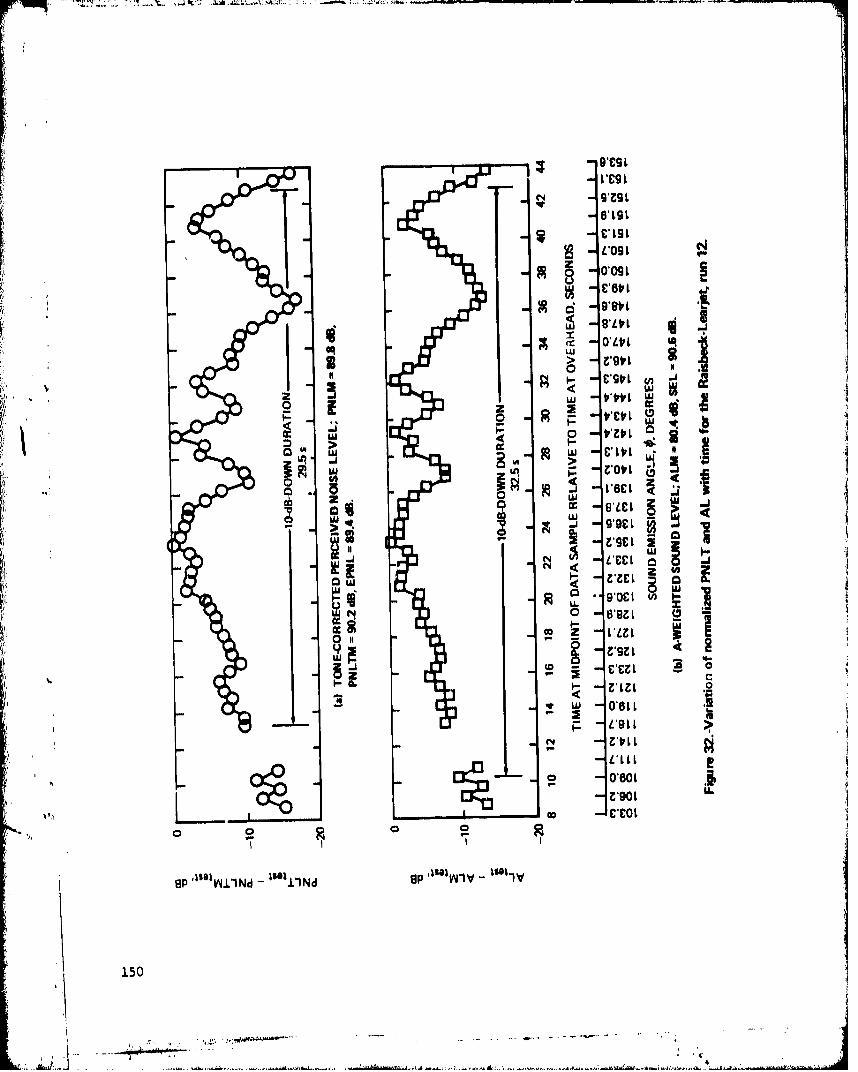
C091
0,091
O.V uz
wn w C,I~ D
0 IQ ~a 09
wow
- 4 Z
ivan. I
1500
-91

1/3-Octave-Band Sound Pressure Levels at the Time of PNLPM.-Thus far we
have discussed the time variation of perceived noise level and A-weighted
sound level. We have also discussed tone-correction factors for perceived
noise level and the duration factors in the calculation of effective per-
ceived noise level and sound exposure level. We now turn to the 1/3-octave-
band sound pressure level spectra.
The sound pressure levels at the time of occurrence of PNLTM are shown
in Fig. 33 for all nine test cases.
The spectra for the four DC-9 runs that were at the same nominal heightover the microphone (at the distance designated AMH in the legends for the
figures) are shown in Fig. 33(a). The propagation distances, PD, and sound
emission angles, 4, are tabulated in the legend. Note that the low-frequency
component of the spectrum is significantly lower for run 322 than for the
other three runs because run 322 was flown at a lower power setting (see
Table 4). All runs had a spectral peak in the band at 3150 Hz.
Note also that the high-frequency sound pressure levels in the 4000 to
10,000-Hz bands were significantly lower for run 272 than for the other three
runs. The lower levels are probably the result of more-absorptive conditions
along the sound path at the time of run 272 because, as shown in Figs. 25(a)
and 25(b), the atmosphere was considerably drier during run 272 than during
the other runs. The adjustment factors from test-to-reference conditions
should therefore be greater for run 272 than for the other runs in Fig. 33(a).
Figure 33(b) shows the spectra for DC-9 run 374 and for the 727. Those
two runs were flown at about the same height overhead, but the propagation
distances and sound emission angles were different becaise the 727 was
climbing while the DC-9 was flown in a level flight path. The emission
angles also differ because the 727 was at takeoff power instead of the
reduced power setting used for the DC-9 runs. Note the much higher level of
low-frequency jet noise for the 727 even though the propagation distance
was 507 m compared with 369 m for the DC-9. The 727 and the DC-9 are
both powered by JT8D turbofan engines.
151

I.80
RUN AMH, PD,NO. m m deg
70 0 0 272 155,8 159.5 102,3
S03 322 153,8 156.8 101.3" 358 152,8 154.4 98.2
S378 156.8 162.3 105.0
;60
(a) DC.9-14 AT OVERHEAD HEIGHTS FROM 152.8 m TO 156.8 m.
110
-o
w"- 100wI~
90"0 90z
8S' 80
70
60 RUN AMH, PD,
NO, m m deg EPR
"O B-727 25 334.8 507.2 139.5 T.O.
o DC-9 374 339.8 369.4 113.1 1.44,, •5 0 i I i I i a a I i I I I I I i I i I I I I I
50 50 80 125 200 315 500 800 1250 2000 3150 5000 800060 100 160 250 400 630 1000 1600 2500 4000 6300 10,000
1/3.OCTAVE.BAND CENTER FREQUENCY, Hz
(b) 727.100 AND DC-9-14 AT OVERHEAD HEIGHTS OF 334.8 m AND 339.8 m;
NOTE DIFFERENT POWER SETTINGS.A.
Figure 33.-Aircraft sound pressure level spectra at the time of occurrence of themaximum test-time tone-corrected perceived noise level, PNLTMtest.
"152Aj
S. . . .•: .. .. ,,,•,V.,,• .,.d~a '•.,, ,•, . ... . .-. . . " .

[,i
90
-$ . 80 "
so
wu 70
w
Uj 60CL
z
00•}, ~50-
RUN AMH, PD,I•, ~40...
4 0 LEARJET 12 1357,8 1925.7 135.203 HS.748 7 657.8 652.5 92.1SBEECH 119 296.8 298,9 83.2
3050 80 125 200 315 500 800 1250 2000 3150 5000 8000
63 100 160 250 400 630 1000 1600 2500 4000 6300 10,000
1/3.OCTAVE.BANO CENTER FREQUENCY, Hz
(c) LEARJET, HS.748, AND BEECH DEBONAIr4.
Figure 33..Concluded.
153
Sit.,
Figure 33(c) presents the spectra for the Raisheck-LearJet (the run with
the longest propagation distance at 1925.7m) and the two propeller-powered
airplanes thc Hawker Siddeley HS-748 and the Beech Debonair. The strcng
spectral peaks in the HS-748 spectra in the 100, 200, and 400-Hz bands are
related to the fundamental and harmonics of propel blade.-passing frequency.
The spectrum from the Beech Debonair did not contain the sharp spectral peaks
that the HS-748 spectra centained.
The spectra in Fig. 33 illustrate some of the missing-band problems
discussed in an earlier part of this Section. Data for the 63-Hz band are
missing from the DC-9 data in Fig. 33(a) leaving an isolated sound pressure
level in the first band at 50 Hz. Data for the 80-Hz band is missing from the
DC-9 spectra for run 374 in Fig. 33(b). Data from the runs with long propa-
gation distances have several band levels missing because of background noise
contamination, espccially in the high frequencies where the effect of atmos-
pneric absorption ha3 reduced the signal to a very low level. The Learjetrun is also missing low-f~-uency data in the 50, 63, and 80-Hz bands.
SThe spectrum for the 727 for the bands at 4000 and 5000 Hz also seems
to indicate the problem of inadequate rejection in the filter stopbands that
was discussed In the ;u.x'-ious Section. On the basis of the 507-ni pathlength
and tihe relatively !,•orptive conditions at the surface, the spectral slope
should h:1ve continued to decrease from the 3150-Hz to the 4000-Hz to the
5000.-Hz bands. The increase rather than decrease in slope is similar to the
filter effect shown, for example, in Figs. 19 and 22.
The ensuing discussion of atmospheric-absorption effects will concentrate
on the four DC-9 runs at the same nominal power setting (omitting run 322)
and the iLearjet, run 12. The adjustments for the 727 and the HS-748 are
not too intcresting because only surface meteorological data were measured.
The adjustments for the Beech Debonair are also not very interesting because
inert'orological data were measured only at the surface and at tne airplane and,
as shown in Table 3, there was not much difference in temperature or humidity
betweel th.' two heights. Also, for the Beech data, because the temperature was
only I1 to 20 C less than the reference Lemperature of 250 C, though the rela-
"l5i1

• | . ...... • '• . .. ... ;'• .. .. .. 7-.... .......... ...
tive humidity was less than 70 percent, the magnttude of the spcctral adjusLmsouiLs
would probably be relatively small. Therefore, because conditions along the
sound propagation paths were not measured during the Beech Debonair tests,
discussion of the effects of the alternative adjustment procedures on the
1/3-octave-band sound pressure levels is omitted for the Beech Debonair data
as well as the 727 and HS-748 data.
Atmospheric Sound Absorption Coefficients.-One of the objectives of
this Study was an evaluation of the differences in calculated band-level
Sadjustment factors caused by differences In computing atmospheric absorption
by the method in SAE ARP866A and that in ANSI S1.26-1978. To anticipate
V• • the magnitude and ,tign of the differences, Fig. 34 shows how the atmospheric
sound absorption coefficients from the two methods vary with the frequency of
a sound wave and the relative humidity and temperature of the air.
The absorption coefficients for the ANSI S1.26-1978 method are presented
as a smooth continuous function of frequency In accordance with the method
in the Standard. However, the coefficients for tOe method of SAE ARP866A
have a discontinuity at 5000 Hz [see, in particular, Fig. 34(h)]. The dis-
continuity, while it could have been eliminated by just using the equations
for the method and simply varying the frequency in regular steps, was included
in Fig. 34 because the discontinuity is a central part of the method of
SAE ARP866A when dealing with 1/3-octave band data. Thus, the absorption
coefficient by SAE ARP866A that is plotted at 5000 H1z was actually calculated
for a frequency of 4500 11z; at 6300 1Iz it was calculated for 5600 Hz; at
8000 Hz it was calculated for 7100 Hz; .-id at i0,00,) !Iz it was calculated
for 9000 11z. The result is a displacet'tent to the right of the high-frequency
end of the absorption-coefficient curve.
It is interesting to observe that a displacement to the left of the high
frequency portion of the SAE ARP866A curves would make them almost coincide
with the high-frequency curves calculated by the ANSI S1.26-1978 method.
Neglecting the built-in differences between the two methods at high
frequencies, the main differences is in the absorption coefficients at low
155

1001 1 1 1 1fi
-ANSI S1,26-1978
SAE ARP866A
E 10
z
0
z0
0
z0
U,
U)
0.1
0.0
40 100 1000 10,000
FREQUENCY, Hz
(a) AIR TEMPERATURE: 50 C.
Figure 34.-Pure-tone atmospheric sound absorption coefficients by ANSI S1.26-1978
and SAE ARP866A.
156

r10. _ ___I' III -. I II I II'
100I If
-I ANSI S1,26-1978
SAE ARP866A
E 10
z
U.~
z -, - //0. - _
cc 1.0 -o -
0C, /
u /,- /
0./o, /
./ ///
"/
0,01 I 1111 I I 1111111 I I 1111II40 100 1000 10,000
FREQUENCY, Hi
(b) AIR TEMPERATURE: 150 C.
-Figure 34.-Continued.
157
. . . . .

100
- ANSI S1.26,1978- -" SAE ARP866A
E 10
o • /zLU
0LU
S0 1 :
• ' .c 0 .0 1j4
0
zo
CYATR
T
a.l15/
0. 011 , 040 1010
10.8

frequencies when the humidity is moderate to relatively high, see Figs. 34(h)
and 34(c). The difference at these frequencies would be most significant
for long propagation paths. In the frequency range from about 500 to about
2000 Hz, the method of ANSI S1.26-1978 generally indicates a smaller absorp-
tion coefficient than the method of SAE ARP866A. Thus, for data in that
range of frequencies, the band-level adjustment factors to reference condi-
tions should be somewhat smaller, for most test conditions, for the method
of the ANSI Standard than for the method of SAE ARP866A.
b
Band-LeveZ Teot..to-Reference-Day Adjustment Factors.-The first set of
1/3-octave-band sound-pressure-level adjustment factors are shown In Fig.
'38 for DC-9 runs 358, 378, and 272. Those three runs had approximately equal.
V• propagation distances and sound emission angles at the time of PNLTM. Also,
they all were flown at nearly equal engine power settings, see Table 4.
K The sound pressure level adjustment factors for the three runs in Fig. 35
are arranged in order ranging from run 358 which had the smallest values for
the test-to-reference-day adjustment factors to run 272 which had the largest
ýi adjustments of the three runs. The fact that the adjustments were largest
for run 272 was expected because the test-time high-frequency sound pressure
levels for that run were significantly lower, as shown in Fig. 33(a), for
that run than for runs 358 or 378. Also, on the basis of the low temperature
and low humidity during run 272 [see Figs. 24 (a) and 2 5 (a)], it was expected
that the adjustments to 250 C and 70 percent relative humidity should have
been relatively large for the data from run 272.
The fact thati the adjustments were somewhat larger for run 378 than for
run 358 was expected because, again as shown in Fig. 33(a), the test-time high-
frequency sound pressure levels were lower for run 378 than for run 358. For
the same propagation distance, emission angle, and engine power setting, the
lower values of sound pressure level should have been associated with a larger
amount of atmospheric absorption along the sound path. Thus, the lower values
of sound pressure level should have the larger adjustments to reference meteor-
ological conditions.
159
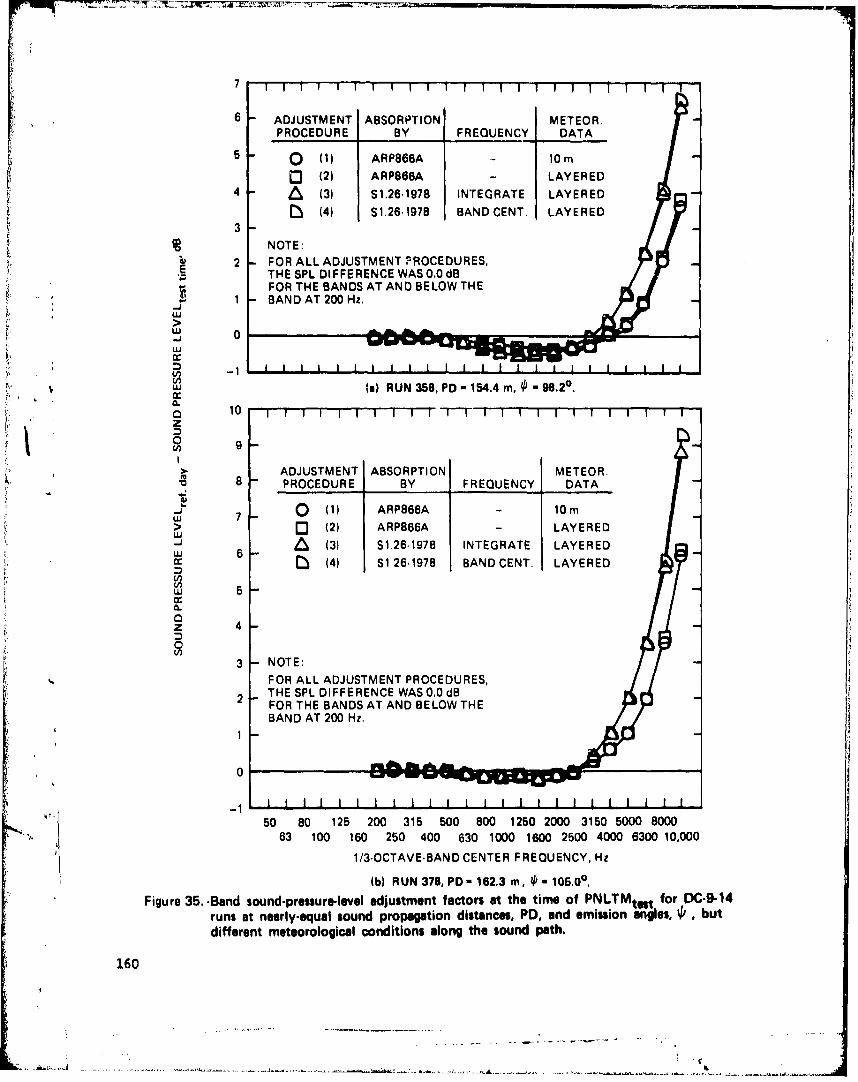
6 ADJUSTMENT ABSORPTION METEOR.PROCEDURE BY FREQUENCY DATA
5 ( (1) ARP866A 10MC (2) ARP866A - LAYERED
4 & (3) S1,26.1978 INTEGRATE LAYERED
( J (4) S1.26.1978 BAND CENT. LAYEREDS3
SNOTE:2 FOR ALL ADJUSTMENT PROCEDURES,
THE SPL DIFFERENCE WAS 0,0 dBa - FOR THE BANDS AT AND BELOW THE
1 -BAND AT 200 Hz.-"JLU
-J 0LUJ
'T'7
' (a) RUN 358, PD = 154.4 m, P u 98,2(.
o, 10 /i-i-'T ! I i I I i 1111I I
z0
ADJUSTMENT ABSORPTION METEOR.8 PROCEDURE BY FREQUENCY DATA
w 7 0 (1) ARP866A - 0MQ> (2) ARP866A - LAYEREDSI.U
w 6 A (3) S1.26-1978 INTEGRATE LAYEREDi (4) S1.26.1978 BAND CENT, LAYERED
Z 4
3 NOTE:
FOR ALL ADJUSTMENT PROCEDURES,2 THE SPL DIFFERENCE WAS 0.0 dB
FOR THE BANDS AT AND BELOW THEBAND AT 200 Hz.
0 ""
50 80 125 200 315 500 800 1250 2000 3150 5000 80001 63 100 160 250 400 630 1000 1600 2500 4000 6300 10,000
1/3-OCTAVE-BAND CENTER FREQUENCY, Hz
(b) RUN 378, PD - 162.3 m, 4 105.00.
Figure 35.-Band sound-pressure-level adjustment factors at the time of PNLTMtest for DC-9-14runs at nearly-equal sound propagation distances, PD, and emission angles, 4, butdifferent meteorological conditions along the sound path.
160

16
15
14SADJUSTMENT ABSORPTION METEOR.
13 PROCEDURE BY FREQUENCY DATA
0 (1) ARP866A - lo1m12 - (2) ARP866A - LAYERED
u (3) S1.26.1978 INTEGRATE LAYEREDU 1 (4) S1.26.1978 BAND CENT. LAYEREDUJ
M 10S/9
z• 8
> 7.
NOTE:,,; ..a 6 - FOR ALL ADJUSTMENT PROCEDURES,
THE SPL DIFFERENCE WAS 0.0 dB FORuJ THE BANDS AT AND BELOW THE BANDS•- AT 200Hz.
r% 4-
4
S 3 --z
2
0
t- 1I
50 80 125 2AJ 315 500 800 1250 2000 3150 5000 800063 100 160 250 400 630 1000 1600 2500 4000 6300 10,000
1/3-OCTAVE-BAND CENTER FREQUENCY, Hz
(c) RUN 272, PD - 169.6 m, . 102.30.
Figure 35.-Concluded.
161
The reason the test-time atmospheric conditions should have been more
absorptive for run 378 than for run 358 is not obvious from inspection of the
meteorological data in Figs. 24 and 25. It is noted, however, that the pro-
files of the molar concentration of humidity in Fig. 25 had a negatite lapse
rate for all runs [including the Leariet run in Fig. 25(c)] except run 358
for the range of heights between the surface and the height of the airplane.
For run 358, the lapse rate of humidity was powitive, as was the temperature
-i lapse rate shown in Fig. 24(c). Apparently, the meteorological conditions
along the path kept changing in such a way that the test-time absorption loss
was closer to the absorption loss under reference conditions for run 358 than
for run 378.
The data shown in Fig. 35 Jillustrate some general trends observed for the
"six of the nine test cases where meteorological data were measured along the
sound propagation path. First, therewas some frequency below which the test-
to-reference adjustment factors equalled zero decibels (actually less than
.0.05 dB because of rounding to the tenth of a decibel In the calculations).
T..he frequency below which the adjustment factor was always zero decibels was
a function of (1) which model was used to calculate atmospheric absorption
losses, (2) the meteorological conditions at the time of the test, and (3)
Cj the length or' the propagation path. In general, the frequency above which
ithe adjustment factors were always nonzero was higher using the ANSI S1.26-1978
""; ethod thUM the ,iicthod of SAIF. ARIP866A, i.e., by adjustment procedures (3)
or (4) than by procedures (1) or (2).
This result is con.;fstent with the differences in the low-frequency absorp-
tion coefficientts In Fig. 34. ('ompare, for example, the curves in Fig. 34 (c)
[or the reference temperatnire of 250 c, at frequencies below 500 Hz, with those
-'or colder temperatures in Figs. 34(a) or 34(b). The differences arise because
the model in SAE. ARP866A is Independent of humidity at low frequencies for
warm temperatures [25 c'], while the model In ANSI S1.26-1978, which is based
" on an Improved understanding of absorption mechanisms at low frequencies, indi-
cates a strong dependence on humidity at all temperatures. The consequence
of the differences in the low-frequency absorption losses calculated by the
two models is not large In an absolute sense unless the propagation path is
of the order of thousands rather than hundreds of meters.
.162

•i The second interesting feature of the band-level adjustment factors inFig. 35 is that over a relatively large frequency range (generally from 250
to 2000 Hz in Fig. 35) the adjustment factors are negative rather than positive.
A negative factor indicates that the sound pressure level under reference con-
ditions is lower than under the test-time conditions, i.e., that the test-time
meteorological conditions are less absorptive than the reference conditions.
Although, as can be seen from the data in Fig. 34 or by examination of the
tabulated values of absorption coefficients in Volume III of this report, the
absorption coefficients for the warm and humid conditions at 250 C and 70-per-
cent relative humidity are usually smaller than for other temperatures or hum-
idities, they can be greater at some frequencies. At high frequencies, the
reference-day absorption coefficients are almost always smaller than those under
practical test-time conditions with the result that the adjustment factors
are generally positive at high frequencies and the sound pressure levelws are
greater for reference than for test-time conditions.
The magnitude of the negative adjustment factors was always less than one
decibel for the pathlengths corresponding to the data in Fig. 35. Longer path-
lengths would be expected to result in calculation of factors that are more
negative than those for the pathlengths of Fig. 35. The importance of negative
adjustment factors is that they tend to offset, to a degree, the influence of
positive adjustment factors at high frequencies. For a particular aircraft,
thu. net effect on perceived noise level or A-weighted sound level. depends on
the shape of the spectrum of the sound signal at the microphone. For aircraft
that produce a spectrum having a large amount of liw-frequency energy, for
example the Learjet at takeoff power as in Fig. 33(c), the offsetting effect
of the negative adjustment factors could yield a lower, rather than a higher,
reference-day EPNL and SEL compared with the test-time values.
For most aircraft noise-certitication tests, the relatively small, negative
adjustment factors will not be large enough to offset the larger, positive,
high-frequency adjustment factors. Hence, reference-day EPNLs will usually
tend to be greater than test-time EPNLs. It may be significant, however, to
note from Fig. 35 that the method of ANSI S1.26-1978 [procedures (3) and (4)]
produced mid-frequency adjustment factors that were consistently more negative
than those calculated using the method of SAE ARP866A [procedures (1) and (2)].
1.63

The most-significant feature of the data in Fig. 35 is the large and
positive values of the adjustment factors in the higher-frequency bands starting,
approximately, in the 2000-Hz band for the pathlengths of Fig. 35. The magnitude
of the adi ustinent factor, Lu a particular high-lrequency band, increnasd as th,
test-time meteorologi.cal conditions became increasingly more absorptive, i.e.,
from run 358, to 378, to 272. The frequency where the adjustment factor changed
from negative to positive decreased as the test-time conditions became more
absorptive.
Of greater interest, however, are the differences between the sole use of
meteorological conditions at the 10-m height, procedure (1), and the use of con-
ditions along the path in a layered-atmosphere analysis, procedure (2). On the
V basis of the differences shown in Fig. 24 in test-time absorption coefficient
at 3150 Hz over the height range, it was not expected that there would be large
differences [or the DC-9 runs between using 10-m and sound-path meteorological
cond Li ions. That expectation was confirmed by the results in Fig. 35 where the
difference in band-level adjustment factor between the methods of procedures
(1) and (2) was no more than 0.5 dB at 1.0,000 Hz for the more-absorptive condi-
tions of run 272, Fig. 35(c). The longer-pathlength and very-absorptive
conditions for the Learjet test, see Fig. 24(f), should show more influence of
the effect of the choice of test-time meteorological conditions than any of
the DC-9 runs.
For data in Fig. 35, however, high-frequency band-level adjustment factors
calculated using only 10-m meteorological conditions were always smaller than
those calculated using the sound-path conditions for the layered-atmosphere
analysis of procedure (2). This result is expected to be applicable to most
aircraft noise test conditions likely to be encountered in practice because
meteorological conditions aloft are generally associated with larger test-time
sound absorption coefficients than test-time conditions at 10 meters above the
ground surface.
Another feature of the results in Fig. 35 is that, as expected, the adjust-
ment factors for the high-frequency bands are larger when calculated using the
atmospheric-absorption model of ANSI S1.26-1978 than using the model of SAE
ARP866A. For center frequencies between 4000 and 10,000 Hz, the difference
164

ranged from less than 0.5 dB to as much as 5 dB at 10,000 Hz for the absorptive
test-time conditions of run 272.
Most of the difference between the results obtained using the two models
can be attributed to the use of the lower bandedge frequency in the SAE ARP866A
procedure to represent the loss over the four 1/3-octave-bands from 5000 to
10,000 Hz. In fact, if the dashed lines in Fig. 34 representing the SAE ARP866A
model were to be shifted to the left by an amount representing the ratio of the
center frequency to the lower bandedge frequency, the resulting band-adjustmenti factors would be in closer agreement than they are in Fig. 35.
The change from using the band center frequency to using the band lower
cutoff frequency introduces a kink or discontinuity in the adjustments calcu-
lated using the SAE ARP866A model in procedures (1) and (2). The discontinu-
ity occurs between the bands at 4000 and 5000 Hz and is most easily seen for
the results in Fig. 35(c).
One final remark from the results in Fig. 35 is that the band-center-
frequency method of procedure (4) always produced a somewhat larger adjustment
factor for the high-frequency bands than did the band-integration method of
procedure (3). The difference increased as the slope of the high-frequency
portion of the test-time spectrum became steeper with increasingly more-absorp-
tive test-time conditions. For the data in Fig. 35, there was no difference in
adjustment factors by procedures (3) and (4) for band center frequencies up to
5000 Hz. The larger factors calculated by the band-center-frequency method for
spectra with steep high-frequency slopes and the agreement at low frequencies
are both consistent with the results obtained by Montegani21 and with the results
of the analytical study in Section 2, see Fig. 14.
For spectra containing steep negative slopes in the high-frequency bands,
the adjustment calculated by the band-integration method is intrinsically more
correct than the adjustment calculated by the band-center-frequency method.
Unless one has available aircraft noise data measured at different dis-
tances under reference meteorological conditions and under a variety of test-
time conditions and were able to compare the ability of the various procedures
165
to adjust the measured non-reference-condition data to the measured reference-
condition data, there does not seem to be any analytical technique to use air-
craft noise measurements for determining the absolute accuracy of any particular
adjustment method. Indeed, aircraft noise data may well be the poorest choice
for trying to make such a judgment because of the difficulty of trying to assure
repeatability for those physical parameters which can be controlled as well as
repeatability of the atmospheric parameters which can be measured, not controlled.
Pernet , in a review of aircraft noise propagation literature for the NationalPbysical Laboratory, has described measuring techniques which should be improved
in order to make better use of aircraft noise measurements for understanding
aircraft noise propagation phenomena.
Mueller and Hilton 23 conducted an analysis similar to that described aboveusing data extracted from the same series of DC-9 tests in 1974 at Fresno Air
Terminal and at Yuma International Airport. They considered adjustments to
sound pressure levels obtained during tests under three differei~t test conditions
at Fresno [none of which was among those analyzed here] and to ,,ound pressure
levels obtained at Yuma under nearly constant temperature and humidity conditions.
The Yuma tests were considered to represent reference data. Because of background
noise, they had no data in the bands from 5000 to 10,000 Hz.
They used absorption-loss models of SAE ARP866A and ANSI S1.26-1978. An
undefined "bandwidth correction procedure" was developed and used with the model
of ANSI S1.26-1978 to give a quasi band-integration procedure for calculating
an adjustment factor from test-to-reference conditions.
Mueller and Hilton concluded that the mzthod based on ANSI S1.26-1978 gave
results closer to the measured reference data than did the method Lased on
SAE ARP866A. They also concluded that an adjustment mcthod using a layered-
atmosphere analysis gave results closer to the mea*iured reference data than
the method based on using only meteorological data measured at a height of
10 meters.
The study reported here does not provide any fundamental data for assessing
the validity of the atmospheric-absorption model of ANSI S1.26-1978 over that
in SAE ARP866A. The study does provide data that can be used to evaluate the
166

magnitude of the differences in test-Lo-reference-day hand-level adjustment
factors and the resulting changes in IPNJ, PNLT, E[PNI., AL, and SEL.
Figure 36 presents a comparison of the sound pressure levels calculated
for the 250 C, 70-percent-relative-humidity acoustical reference day acc rding
to procedures (2) and (1) for runs 358 and 272. Procedures (2) and (3) both
used sound-path weather. Procedure (2) used SAE ARP866A. Procedure (3) used
ANSI S1.26-1978.
For the relatively short propagation distances at the time of I'NLTM for
these runs, the differences between the spvr.tra for the two runs In Fig. 36
are not consit 4 d significant for band center frequencies at and below 31.50 ilz.
l)ifferences between the spectra in the four bands from 5000 to 10,000 Htz are
considered to be sIgnificant in that they illustrate the influence of the two
atmospLIeric-absorpttoit models.
If all other factors involved in a measurement of aircLaft noise (engine
power setting, airspec, propagation distance, sound emission angle, wind,
atmosoheric turbulence, and so forth) are equal, then a reference-day spectrum
calculated from one set of Lest-time data should be the same as another refer-
('010,.-day spectrum calculated from another set of test-time data. This rationale
was the basis for comparing the reference-day spectra from runs 358 and 272 in
Fig. 36. The other factors were as close as the available data permitted.
Therefore, on thaL basis, the atmospheric-absorpt ton adjustment procedure
that yielded the smallest set of differences between the two reference-day
spectra could be considered superior to other adjustment prcceduress. For the
four bands from 5 to 10 kflz, inspection of the data plotted Fig. 36 shows
"a closer grouping of the reference-day band levels by procedure (3) [Fig. 36(b)]
than by procedure (2) [Fig. 36(a)]. The evidence indicates a preference for the
atmospheric absorption model of ANSI S1.26-1978 over that in SAE ARP866A. Because
"of the relatively short propagation distances, the differences shown ini Fig. 36.•. *,
between the two procedures were not large although they appear to be consistent.V~ 23
The trends agree with those observed by Mueller and Hilton
The reference-day sound pressure levels in the 5 to l0-kHz bands by pro-
167
- . ---A- 4 ii

70 "0 RUN PD, 4, PN LTref EPNLref
NO. An deg d8 dB
..J 358 154.4 98.2 111.9 106.0Ii •u~2"72 159.5 102.3 11. 10.
,,, 60 1
(a) PROCEDURE (2): SAE ARP866A. CENTER FPIEQUENCY EXCEPT 5 TO 10 kHz.
ZS0 80
I'70 kORUN PD, •, PN LTref EPN Lre,
I NO. m deg dB dB
0 358 1544 98.2 112.2 106.33 272 159.5 102.3 111.5 106.1
601 1 1 11111 1 1 11 1 1 1 1 I III
50 80 125 200 315 500 800 250 2000 3150 5000 8000
63 100 160 250 400 630 1000 1600 2500 4000 6300 10,000
1/3-OCTAVE-BAND CENTER FREQUENCY. Hz
(b) PROCEDURE (3): ANSI S1.26-1978, BAND INTEGRATION.
Figure 36. 1Ilustrrution, for DC-9-14 runs 272 and 358, of difference between
-eference-day sound pressure levels calculated by adjustmentprocedures (2) and (3). Propagation distances and sound emissionangles are for thb time of PNLTeItest.
16P

-7 L
cedure (2) are, of course, lower thnn those by procedure (3) because of the
use of the lower bandedge frequency to represent the absorption over the band.
The higher levels in the 5 to l0-kHz bands did not alter the value of the
tone-correction factor calculated for the various spectra in Fig. 36. A 1.8-dB
tone-correction factor was calculated for the reference-day spectra as it was
for the corresponding test-time spectra, see Fig. 31. The band producing the
maximum tone-correction factor was always the band at 3150 Hz. The tone-
corrected perceived noise levels and the effective perceived noise levels for
the reference-day spectra were 0.3 dB greater according to procedure (3) thanprocedure (2), primarily because of the higher sound pressure levels in the
5 to l0-kHz bands by procedure (3).
As the pathlength increases, the magnitude of the adjustment factors
would generally be expected to increase. The data analyzed above had a
pathlength of about 160 m. Figure 37 shows the band-level adjustment
factors from run 374 for a pathlength of about 369 m. The results are similar
to those shown in Fig. 35 except that (1) the first low-frequency band with
nonzero adjustments is now the 125-Hz band instead of the 250-Hz band, (2)
the adjust:-ents in the mid-frequency range have values which are more negative
than any of the corresponding values in Fig. 35, and (3) the high-frequency
adjustments are larger (more positive). There are no data for the band at
10,000 Hz because the test-time sound pressure levels In that 'aid were
missing and hence no reference-day sound pressure levels were calculated.
For the high-frequency bands, the methods of procedures (1) and (2)
again showed that the use of meteorological data at a height of 10 m consis-
teiktly produced smaller adjustments than the use of meteorological data along
the souni pach. The kink that was observed for the results in Fig. 35 in the
slope of the ad,,'i :#nt factors between the bands at 4000 and 5000 Hz for
procedures (1) and ý2) us r., the model of SAE ARP866A is also evident in Fig.
37.
In Fig. 35, there was no difference between adjustment factors calculated
by the band-integration method of procedure (3) and the band-center freqaency
method of procedure (4) except for the very high-frequency bands where the
spectral slope was quite steep. For runs 358 and 374, the smaller adjustments
169

13
m 12
11 ADJUSTMENT ABSORPTION METEOR.PROCEDURE BY FREQUENCY DATA
-J 10 0 (1) ARP866A - 10M
Q [3 (2) ARP866A - LAYERED
,- 9 & (3) S1.26.1978 INTEGRATE LAYERED' (4) S1.26.1978 BAND CENT. LAYEREDUJ
uJ 8cc
r• 7oz0V, S 6
-J NOTE:"w FOR ALL ADJUSTMENT PROCEDURES,> 4u THE SPL DIFFERENCE WAS 0,0dB FOR
"THE BANDS AT AND BELOW THE BANDn: AT 100 Hz.
cc 2
z
0 Il
50 80 125 200 315 5r 800 1250 2000 3150 5000 8000"63 100 160 250 406 -330 1000 1600 2500 4000 6300 10,000
I 1/3 OCTAVE-BAND CENTER FREQUENCY, Hz
Figure 37.-Band sound-pressure-level adjustment factors at the time of PNLTMtestand of ALMtest for DC-9-14 run 374, PD 369.4 m. = 113.10.
170
by the band-integration method were first noted in the 8000-Hz band. For run
272 in Fig. 35(c), the smaller adjustments by the band-integration method were
first noted in the 6300-Hz band. For run 374 in Fig. 37, the even-more-
steeply-sloped high-frequency spectrum of the noise signal after propagation
over the longer pathlength caused the center-frequency method to produce larger
adjustments than the band-integration method starting in the 4000-Hz band.
The largest difference, however, was about 0.5 dB in the 8000-Hz band where
the slope of the test-time spectrum was -8 dB/band.
The reference-day sound pressure levels calculated for run 374 can be
used to obtain additional insight into the relative differences between the
atmospheric absorption models of SAE ARP866A and ANSI S1.26-1978. During the
analysis of data acquired from a noise-certification test program, it is often
required that the reference-day results be further adjusted for propagation-
pathlength differences that stem from the actual airplane flight path not
being equal to the flight path calculated for the airplane under the speci-
fied reference conditions. Thus, it is often necessary to include an addi-
tional adjustment factor for propagation over shorter or longer pathlengths.
Adjustment of a sound pressure level spectrum to a longer, or shorter, propa-
gation distance is also required when generating predictions of aircraft
noise levels at large distances, as, for example, in determination of the
data base for calculations of the locations of contours of aircraft noise
exposure around airports.
Comparisons of aircraft noise spectra at different distances should be
made at the same sound directivity angle because the spectrum can change rela-
tively rapidly with angle. For the data available for analysis, reference-day
spectra were only produced for two sound emission angles (i.e., for two times).
The angles were those associated with the time of occurrence of PNLTMtest
and ALMt . For run 374, the two maximum values both occurred at an angle oftest'
113.1°. For the three runs at the shorter distance and at the power setting
used for run 374 (namely, runs 358, 378, and 272), the angle at the time of
PNLTM was less than the angle at the time of ALMs. From Table 5(b),test test'
we see that runs 358 or 378 could be used to provide data at an angle close
to the 113.10 angle of run 374. For run 358, the emission angle at ALMtest
171

was 110.50, for run 378 it was 115.8*. We chose run 358 t provide a spectrum
to compare with run 374 because, as shown in Fig. 35, the test-time meteorolo-
gical conditions were closer to those for an acoustical reference day than
were those for run 378.
Figure 38 shows the measured test-time and the calculated reference-day
spectra for runs 358 and 374. The results obtained using the model of SAE
ARP866A are presented in Fig. 38(a); those obtained using ANSI S1.26-1978 are
* shown in Fig. 38(b). The generally similar appearance of the spectra from
the two runs is another indication of the good reproducibility of the data
S' from these 1974 FAA/NASA flyover noise tests.
For constant directivity angle, the process of extrapolating a sound
* pressure level, in sone band of frequencies, from distance sI from the source
to a larger distance s2 can be represented analytically by
• •L2 - Ll - 20 log (s2/sl) - Aa (93)where the -20 log (s 2 /s 1 ) term accounts for inverse-square divergence loss Iunder the assumption that sound waves spread spherically outward from aneffective acoustic source and the A term accounts for losses resulting from
aatmospheric absorption.
For propagation outward from a source, the atmospheric-absorption-loss
term for sound analyzed by ideal filters can be represented by the following
general expression*
fI
A -10 log [ [exp(J 2 2a ds)] df .G. R d (94)
ff L Rl J
where, as before, Gl represents the pressure spectral density of the sound as
a function of frequency at a receiver location at distance sl and a is the
atmospheric absorption coefficient as a function of frequency. The coefficient
a in Eq. (94) has units of nepers/meter for distances in meters.
*See Eq. (A2) of Ref. 2.
172
L ......... _ .....

80
70-
S RUN met. PD, ,NO. cond., m dg
0 3 eis 163.2 110.5
S374 test_ J374 ref. 369.4 113.1w 50
s() BAND.LEVEL ADJUSTMENT FACTORS BY PROCEDURE (2W,SAE ARP566A, CENTER FREQUENCY EXCEPT 5 TO 10 kHz.
0..9090
U,00
NO. cond. m deg
60 358 test 1 "358 ref. 6.,1.
S374 test 3[3 374 ref. 369.4 113.1
5050 80 125 200 315 500 800 1250 2000 3150 5000 8000
63 100 160 250 400 630 1000 1600 2500 4000 6300 10,000
1/3.OCTAVE.BAND CENTER FREQUENCY, Hz
(b) BAND-LEVEL ADJUSTMENT FACTORS BY PROCEDURE (3),ANSI S1.26-1978, BAND INTEGRATION.
Figure 38.-Sound-pressure-level spectra for test and reference meteorological
conditions from DC.9-14 runs 358 and 374 at nearlylequal sound-emission angles but different propagation distances.
173
•"I
Over the frequency range of the filter from fL to fu, evaluation of the
integral in the numerator of Eq. (94) requires a separate evaluation at each
frequency of the integral in the exponent of the exponential term because the
absorption coefficient A is also a function of temperature, pressure, and
humidity and those meteorological parameters may not be constant along the path
from distance al to distance s2. Evaluation of the integral over the path
from si to S2 for the exponential term requires knowledge of the variation of
temperature, pressure, and humidity as a function of distance along the path.
In practice, the path would be divided into segments over which average condi-
tions were known and the integral would be replaced by a summation as done
for Eqs. (80) and (81).
P. If the meteorological conditions were constant over the path (as they areiVfr the acoustical reference-day conditions in the current version of FAR 36)
1 then, as for Eq. (21), the absorption-loss expression of Eq. (94),
for constant reference conditions, becomes
SAafref -1-i0 log GR-
G[ u d (95)
where (s2 - s5) is the pathlength and a is the absorption coefficient forrefconstant reference meteorological conditions in units of decibels/meter as a
function, now, only of frequency.
As a further simplification, if the sound is a pure tone at some frequency
between f1 and f or if the absorption loss is being calculated by treating the
pressure spectral density of a broadband sound analyzed by a bandpass filter
as though it were a pure tone sotund, then Eq. (95) reduces to
A r (ar)(s 2 - S) (96)a,ref ref
where a ref is at some frequency within the frequency band associated with Aaref.
174
• ,. I "

Because the method of SAE ARP866A uses a single frequency to approximatte
the absorption loss over a frequency band, Eq. (96) was used to approximate the
absorption-loss term in Eq. (93). For constant reference conditions along the
sound path, the general expression In Eq. (93) thus becomes
L -LL - 20 log (s?/sj) - (ae)[8s - s0)/100] (97)2,ref lref
where a factor of 100 has been introduced in the absorption-loss term because
a now has the more-convenient units of dB/(l00 m) instead of dB/m.ref
The use of the format of Eq. (97) to project a spectrum from one distance
to a larger distance permitted a direct comparison of the two atmospheric absorp-
tion models as well as the different methods [as used in procedures (2) and (4)]
of approximating the absorption losses for the 1/3-octave bands with center fre-
quencies from 5000 to 10,000 11z.
For the sound pressure levels Ll ref in Eq. (97), we take the spectra
shown in Fig. 38 for run 358 as calculated for referoece conditions. Equation
(97) was used to project the reference-day sound pressure levels of run 358
to the 369.4-m distance of run 374. The difference between the sound pressure
levels projected using run 358 data and the data calculated for run 374 is
then a measure of validity of tOe eytrapolation proceduie. If there is no
difference between the l-,iels projected from run 358 and those calcul.ated for
run 374, then the extrapolation .method is capable of duplicating the data at
the larger distance. Negative values fur the difference mean that the extra-
polation frnm rtin 358 underpredicted the levels from run 374, and vice versa.
The differences t.etween the ba.nd levet- projec:ted from run 358 and those
from ran 374 are shown in rig. 39 as a function of banO center frequency. The
Inverse-square divergence-loss term was a constant 7.! dB 'rom 163.2 to 369.4
meters.
175
•.I

--.. ~
The results in Fig. 39 are shown only for band center frequencies from 800
to 8000 Hz. No data were available for run 374 at 10,000 Hz. There was no dif-
ference between the two adjustment procedures for frequencies at and below 800 Hz.
The general trend shown by the results in Fig. 39 is for the band levels
projected from the 163.2-m distance of run 358 to the 369.4-m distance of run
374 to be about 2 dB lower than those of run 374. The differences in the lower-
frequency bands from 100 to 630 Hz agreed with this trend but ranged from +1.0
to -3.8 dB. The larger scatter in those bands was attributed to differences
caused by variations in the Interference effects resulting from ground rdflec-
tions in the measured test-time spectra for the two rurus.
The reasons the levels projected from the 169.2-m distance for run 358 were
approximately 2 dB lower than those of run 374 over the spectrum fron the 100 to
the 6300-Hz bands are not known. On the basis of the engine and airplane data
listed in Table 4, the strength of the noise at the source should have been nearly
the same for the two runs. The accuracy of the photographic technique for deter-
mining height overhead, however, is about ±5 to ±10 percent. The accuracy of the
time synchronization between the taking of the photograph and the recording of the
noise signal could also account for somp of the 2-dB difference. if the haight at
overhead for run 374 was too large by 10 percent while that for run 358 was too
short by 5 percent, then the inverrse-square-loss term would have been approximately 4
1.3 dB smaller atnd the across-the-speLtrum difference would have beer, reduced to
about 0).7 dB. The small difference in sound emission angle might be able to account
for another 0.2 d3 of the difference because of the differenco in the d!.rectLivity
of the noise at the source.
The most-striking and principal feature of thi results in Fig. 39 is tne
gross difference in thu trends shown for the 5000, 6300, and 8000-11z bands. The
method of procedure (4) based on the model of ANSI S1.26-1978 produced band-level
differences for those bando which were consisternt with r'.L trends observed at
lower frequencies.
176
!'Lk . ": "-- : • - --: .. ,• .

2 I I I ' ! I I I
ATMOSPHERIC ABSORPTION BY:
1 Q (2) SAEARP866A•-.- (4) ANSI S1.26-1978
00
-- 2o-
1 / .4
800 1000 1250 1600 2000 2500 3150 4000 5000 6300 8000 10,000
1/3-OCTAVE.BAND CENTER FREQUENCY, Hz
Figure 39.-For nominally equal sound-emission angles (110.50 and 113.10), illustrationof effect of choice of atmospheric-absorption model on ability to extrapolatereference-day SPLs. Comparision of differences between reference-day SPLsfrom run 358 at 163.2 m extrapolated to 369.4 m and reference-day SPLsat 369.4 m from run 374.
177

S. K_
C' The larger negative value for the 8000-Hz band for procedure (4) is attribu-
ted partly to the use of the band center frequency instead of the band-integration
method and partly (probably mostly) to the suspicion that the test-time sound
pressure level for the 8000-11z band for run 374 was contaminated by power trans-
mitted through the lower stopband. That suspicion is based on the shape of the
high-frequency part of the test-time spectrum showo in Fig. 38 for run 374. Judging
from the absorptivity of the test-time meteorological conditions for runs 374 and
358 and from the roll-off rates for the shorter-distance data of run 358, the test-
time level indicated for the 8000-Hz band of run 374 appears to be higher than
would have been expected.
If the test-time level in the 8000-Hz band for run 374 had been lower, then
the reference-day level would also have been lower and the difference between the.i:;i,' level projected from run 358 and that of run 374 wou~ld have been less i •gative .
(more positive). A change of 2 dB In the 8000-Hz band level for run 374 would
have made the difference at 8000 Hz consistent with the differences in the lower
frequencies for procedure (4).
The differences in the 5000, 6300, and 8000-Hz bands using the SAE ARP866A
model in procedure (2) showed an unusual trend in that the data projected from run
358were greater than the reference-day data from run 374 i" these bands. The
levels in all three of these bands would be larger than those of run 374 if a
reason could be justified for making a 1.5-dB to 2.0-dB net positive adjustment to all
differences in Fig. 39. The fact that the projected data ovwrpredict the reference-
day levels of run 374 is considered to be the consequence of using the lower
b;IndedgL, frequency in SAE ARP866A to represent absorption loss over a band
II ruluei •.y.
Not, 6i1at the dowtr,,:nrd trend from the 6300 to the 8000-Hz bands in Fig. 39
for procedure (2) would have been continued as the steady upward trend from the
4000 to the 6300-liz bands if tile 2-dB reduction in the 8000-Hz reference-day
band level for run 374 was proper as postul ated above in the explanation of
the more-negatLie difference in the 8000-Hz band for procedure (4).
178
Overprediction of high-frequency band levels when using the method of
SAE ARP866A to extrapolate to larger distances is regarded as a significant
shortcoming of the method. If the process had been reversed and the data of
run 374 had been used to estimate the band levels of run 358, the results would
have been reversed and the method of procedure (2) would have underpredicted the
levels of run 358. Errors arising from the use of a single frequency to
calculate atmospheric absorption loss over a frequency band were also pointed
A out by Montegani in Ref. 21.
The conclusion here is that a band-center-frequency or band-integration
method appears to be better able to reproduce high-frequency data measured at
a longer or shorter distance than does the lower-bandedge-frequency method of
SAE ARP866A. Moreover, for all bands between 1000 and 4000 Hz, the method of
procedure (4) with ANSI S1.26-1978 was consistently better (i.e., produced
I7 band-level differences in Fig. 39 that were closer to zero) than the method
of procedure (2) with SAE ARP866A, though only by 0.2 to 0.4 dB. The consis-
tency of the trend and the fact that it was observed in each of the seven bands
between 1000 and 4000 Hz are, however, ccnsidered to be significant factors in
favor of the use of the ANSI S1.26-1978 model instead of the SAE ARP866A model
for atmospheric absorption when adjusting measured test-time sound pressure
levels to acoustical-reference-day conditions. Furthermore, smaller differences
(i.e., improved correlation) would be expected for the high-frequency bands,
where atmospheric absorption effects are most noticeable and the spectral slopes
can be very steep, if the atmospheric-absorption loss were computed by integra-
ting over the response of a filter and if a procedure were used to remove real-
filter effects (i.e., effects caused by non-ideal filter-transmission character-
Istics) from the measured test-time sound pressure levels before adjusting the' data to acoustical-reference-data conditions.
The procedure for removing real-filter effects must, however, be an
approximate one because there is no exact analytical method to determine ideal-
filter band levels from real-filter band levels and the frequency response
characteristics of the filter. /
The analysis of the data from the DC-9 flyover noise tests at Fresno for
propagation pathlengths of about 160 and 370 m has yielded certain conclusions
179
relative to calculation of adjustment factors from test-to-reference meteoro-
logical conditions. The conclusions were concerned with (1) the use of meteoro-
logical data at the 10-m height versue meteorological data along the sound path,
(2) the use of the atmospheric-absorption model of SAE ARP866A versus that of
ANSI S1.26-1978, (3) the use of the band center frequency to calculate
atmospheric-absorption loss versus a method of integrating over the response
of a filter band, and (4) the need to account for real-filter response effects
"in the measured test-time 1/3-octave-band sound pressure levels.
The spectral effects on which the conclusions were based depended on the
length of the sound propagation path and the absorptive character of the atmos-
phere. For the DC-9 runs, the absorptive quality of the atmosphere was not
greatly different from run to run and the pathlengths were relatively short.
For thie one remaining set of flyover noise data with meteorological data avail- iable along the sound path (i.e., that from the test of the Raisbeck-modified
Gates Learjet in run 12), the atmosphere was much more absorptive and the 1926-mr
pathlength was much longer. Differences between the four adjustment procedures
were expected to be larger for the Learjet data than for the DC-9 data.
Figure 40 shows the band-level adjustment factors calculated for the data
from the Raisbeck-Learjet test by the four alternative procedures. The results F
in Fig. 40 apply to adjustment of the test-time spectrum associated with both1PNLTM and ALM since the maximum values of both ,ruantities occurred at
test test;the same relative time (i.e., the saine sound emission angle). The results in
Fig. 40 are limited to band center frequencies from 100 to 3150 Hz because of
background noise contamination of the test-time sound pressure levels in theA low- ind high-frequency bands,
Differences among the four alternative adjustment procedures that were
seen in the results from run 374 in Fig. 37, in comparison with the results for
"the other DC-9 runs in Fig. 35, are much more evident for the results in Fig. 40.
The low-frequency band where the adjustment was zero for all procedures was not
determined hcause it was at a frequency below the limit of the data at 100 Hz.
Differences between the mcthods based on SAE ARP866A (procedures (1) and
(2)] and the methods based on ANSI S1.26-1978 [procedures (3) and (4)1 were
180
0 Noma..... ~,.---.-

20
19
18 ADJUST. ABSORPTION METEOR.PROCED BY FREQUENCY DATA
17 Q - ARP866A ,- 10m
16[ (2) ARPB66A LAYERED
(311 S1.26.1978 INTEGRATE LAYERED
"15 L•(4) S1.26"1978 BAND CENT. LAYERED
"14w
-J13
JJ -12
:311
10CLz 9
0) 8 8• I
"7 NOTE:ADJUSTMENT FACTORS FOR I
6 THE BANDS AT 50, 63, AND
> 80 Hz WERE NOT DETER.5 MINED BECAUbE SPL
,, EQUALED ZERO FORtT4OSE4 BANDS AS WELL AS THE
V)w BANDS AT AND ABOVEu 3 4000 Hz AT THE TIME OF"0~ PNLTMtest AND ALMtest,
z 2
10
-2
% 50 125 315 80G 2C1)IU 500080 200 500 1250 3150 8000
I13 CIrAVE. BAND CENTER FRLiOUENCv,, Hz
Fiuv 40,..Band sound. wessure-level adjustment factors at the time of PNLT t and of ALMtot
for RAisbeck-Learjet, run 12. PD 192t.7 m, P - 135.20,
181
.......... ..-..-. , ." V "'

r• - - i . . - -
particularly ovident for band center frequnncles rrom 100 to .160()0 IIz. Iroi
100 to 400 Hz, procedures (3) or (4) showed postit-ve adjustmwnt factors; eLwen
500 and 1600 Hz, the adjustments decreased to relatively large negat've values.
The adjustments by procedures (1) and (2) were always negative over this fre-
quency range, but not as negative as those calculated by procedures (3) and
(4). The same trends for the differences between the two absorption models
were also in the results from run 374 in Fig. 37, though not as prominent as
in Fig. 40. The differences in adjustment factors are the result of differences
between the two models for atmospheric absorption as shown by the curves in
Fig. 34.
Comparing the results using procedures (I) and (2), Fig. 40 shows that, as
expected, sole use of meteorological data measured at the 10-m height results in
significantly smaller adjustments than use of meteorological data measured along
the sound path. The meteorological conditions aloft [see Figs. 24(f) and 25(c)]
were quite different, and more absorptive, than the conditions at the 10-m height.
Since FAR 36 requires measurements, at various times throughout each test day,
of the meteorological ýonditions of the atmosphere at various heights above
ground level, it would appear to be iogi,:al, and for no significent increase
in test cost, to always use the meteorological conditions along the sound path
when computing adjustment factors for ditferences in atmospheric absorption
under test and reference conditions.
Referring again to Fig. 40, the frequency where the higher-frequency adlust-
ment factors changed from negative to positive was significantly lower than for
the shorter-pathlength adjustment factors shown in Figs. 35 and 37. For pro-
cedure (2) using SAE ARP866A, the crossover frequency was between the 1000-
and 1250-Hz bands. For procedures (3) and (4) using ANSI S1.26-1978, the
crossover frequency was between the 1600- and 2000-Hz bands.
If we consider just the methods that use the meteorological conditions
aloft [procedures (2), (3), and (4)], it is interesting to note that the
adjustments calculated using the procedure of SAE ARP866A were greater (i.e.,
more positive) than thoce calculated using the procedure of ANSI S1.26-1978
for every band center frequency from 630 to the upper limit of the data at
3150 Hz. The effect of the offset or kink in the procedure of SAE ARP866A
182

between the 4000 and 5000-Hz bands is not evident in Fig. 40 because the %tata
terminate at the 3150-Hz band. The adjustments calculated by making use -J
the SAE ARP866A method (i.e., the greater absorption losses) were larger
than those calculated using the method of ANSI S1.26-197B because the absorp-
tion coefficients -t ARP866A are larger at those frequencies than the absorp-
tion coefficients from ANSI S1.26-1978 fur the cold and dry conditions pre-
vailing at the time of the test.
As a final observation about the results in Fig. 40, we note that the
difference between the adjustment factors calculated by the band-integration
method of pro~cedure (3) and the band-center-frequency method of procedure (4)
was small-to-negligible for all frequency bands covered by the available dalta.
The largest difference was 0.5 dB In tle highest-frequency band at 3150 1iz
whrQ the test-time spectral slope was also steepest and the band-ce.nCl.r-Frt-
quency method probably overestimated the actual absorption loss.
.1
A1
183

Ejfet of Differqen (i ae. t Pro10 dourle c. . "So0nd Prb turete
Leve ula.-The discussion of the effoect on the s /u3-,re l,,var ' o iabld pre, sure levels
of using different procedures to calculate adjati-,ic * o-r atmospheric
absorption losses concludes with exam(nati)n of the thigh- red reference-day sound
pressure levels in Fig. 41 at the time of PNL'the Asp r u or the Rme isbeck-Learjet data, Only reference-day levels by procedu i.s (i1), (z), and (3) are
shown because the levels by procedure (4) wer 1 almost identical to those by
fynprocedure (3).
rAt ow frequencies (o.eh , the l00 to Ovr-Hz bands), the differences between
the calculated reference-day sound pressure luvels are noticeable, but not too
S importanth The diffarences among the higher-frequency sound pressure levels
u(i.e., the 500 to 3150-Hz bands) are significant.
de The relatively small adjustments calculated using the aO-m meteorological
,"data and procedure (I) make the high-frequency reference-day spectrum by that
fprocedure have an entirely different shape than the spectrum determined using
procedures (2) and (3). The method of procedurt (i) essentially preserves the•,..rapid high-frequency rolloff of the test-time spectrum. The absorption-loss
toladJustkelt f ncters determined by procedure (L) are not considered to be a reason-
pabl representation of the actual losses over the 1926-m pathlength for the meteoro-• logical conditions as theý existed -t the time. of the test.
The reference-day sound pressure leve-ls calculated using procedures (2) and
(3) both have a more-gradual high-frequency rolloff than the levels calculated
[i u-sing pro,,'edure (1). The levels determined using ARPS66A are higher than those
=• •determiined ucing ANSI S1.26-1978 because the adjustment factors were greater as
I indicated in Fig. 40.
•' The most-interesting aspect or the results shown in Fig. 41. Is the high-
S"' frequency "turning up" of tlhe reference-day spectra determined by procedures
(2) and (3). The "turning up" ol tlh-e spectra at high frequencies is considered
to likely be an incorrec't rv,,tilc bec'au~e the Lear Jet wa•s operated at a hig~h
power setting and the spectrum measured in the far field at an emission ai.gle of
184

IOU"
gg
80
w 70w
"60
PNLT, AL,
DATE ctB da
50 - tewt time 90.2 80.4o PROC. (1) 90.0 80.0o PROC. (2) 90.9 80.5
I, PROC. (3) 90 7 79.740 I I t I I I _L _i i I I I I i I I I ,I I I i
40 -
50 80 125 200 315 500 800 1250 2000 3150 5000 8000
63 100 160 250 400 630 1000 1600 2500 4000 6300 10,000
1/3 OCTAVE-BAND CENTIR FREQUENCY, Hi
Figure 41. .Sound-pressure-leveI spectra for test and reference meteorologicalconditions for Raioeck.Learjet at time of PNLTMtst or ALMtst,
run 12, PD •1925.7 m,4 m135.20.
185

135* should have been that produced by broadband jet-noise sources in the
exhaust streams from the two turbojet engines. A jet-noise spectrum, with a
maximum occurring between the 200 and 315-Hz bands, would be expected to decrease,
not increase, at high frequencies under any meteorological conditions, especially
for a propagation distance of 1926 meters.
The high-frequency "turning up" of the reference-day sound pressure levels
is more noticeable for the levels determined using procedure (3) than using pro-
cedure (2). For procedure (2), the sound pressure levels in the 2500- and 3150-Hz
b.inds are the only levels that appear to be afft.;ted by the "turning-up" phenomenon
in that the band-level slopes over those bands did rot decrease with increasing
frequency as would be expected for a spectrum produceL' by a jet-noise source. In
other words, the level change from thle 1600-Hiz band to the 2000-14z band was -1.9 dB!
then from tile 2000 to the 2500-1iz band the level change decreased to only -2.0 dBl;
from the 2500 to the 3500-11z band the level change Increased to -0.9 d11inllistead of
decreasing. Even for the minimal absorption conditions associated with 250 C and
70-percent relative humidity, the band-Level slope should continually decrease
with increasing frequency for a pathlength as long as 1926 meters.
For procedure (3), the sound pressure levels in the three bands at 2000, 2500,
and 3150 Hz seem to be influenced because the slope of -2.0 dB from the 1250 to
the 1600-Hz band increases to -1.6 dB from 1600 to 2000 Hz, increases again to
-0.2 dB from 2000 to 2.500 Hz, and increases again to +0.8 dB from 2500 to 3150 Hz.
The "turning up" is more noticeable for the procedure (3) results because the band-
level slope actually becomes positive from the 2500 to the 3150-Hz bands. The trend
indicated by the positive slope is that the level in the 4000-Hz band (had there
been any test-time data at 4000 Hz) would have been quite a bit higher than the
level in the 3150 Hz band, and so on. Such a result would be considered to be
ludicrous for a jet-noise source. Such trends are similar to those obtained for
the hypothetical spectrum considered in Section 3 for filters having non-ideal
response characteristics with the results as shown in Fig. 22.
"Turning up" of reference-day high-frequency sound pressure levels calculated
1y adjusting measured test-time sound pressure levels for differences in atmospheric
absorption losses has been observed by others, e.g., see Refs. 24 to 28. The reasons
put forward to explain the "turning up" of the reference-day sound pressure levels
186
4 I

have included speculations that atmospheric absorption losses were not properly
modeled, that meteoiological conditions along the sound propagation path were
not measured properly or with adequate resolution and hence that the adjust-
ments from test-to-reference conditions could not be expected to apply to the
measured test-time sound pressure leveli41 or that the calculated high-frequency
adjustment factors were too l.arge because they were calculated at a single
frequency that was too high to be representative of the loss over the width
of the higher-frequency bands. The latter concern is the reason the nominal
lower bandedge frequency is used in SAE ARP866A for the four bands from 5000
to 10,000 Hz.
Analysis of DC-9 flyover noise data from the 1974 tests at Fresno and2 5Yima that was performed by McCollough and True resolved the problem of a
high-frequency turning up of the reference-day opectrum by arbitrarily rolling
off the adjusted spectrum starting in the 4000 or 5000-Hz bands. The roll-
off was applied after visual inspection of the adjusted sound pressure levels.The rolloff rate appears to have been -6 dB/band for the 1/3-octave-band data.
The difference in reference-day EPNL between using and not-using the arbitrary
rolloff of high-frequency data was said to be less than 0.5 dB for the path-
length distances that were examined.
Calculated values for the high-frequency sound pressure levels reported
here have not included any arbitrary rolloff. Any single rolloff rate was not
likely to be applicable to all engine power settings and measurement distances.
Nor would a single rolloff rate apply to all sources of aircraft noise. The
requirement to iaspect each spectrum to determine the frequency at which tostart applying the rolloff was considered neither desirable nor compatible with
automated processing of aircraft flyover noise data by a digital computer.
It was considered that the cause of the high-ft-reuency turning up of
reference-day spectra should be determined and a solution developed which could
¾,. be used by a digital compucer when analyzing any set of aircraft noise data.
If as suspected, the fundamental problem was incorrect test-time band levels
because of contamination from power transmitted through the lower stopbands
of the filters, than a method should be developed to estimate what the band
levels would have been if the filters had ideal transmission response charac-
187
JJ

-_ . .M: __._-
teristics. Development of an appropriate method to accomplish that task was
not within the scope of the effort reported here.
Effect of Different Adjustment Procedures on Reference-Day EPNL and SEL.-
Thus far we have discussed the effect of alternative atmospheric-absorptionadjustment procedures on 1/3-octave-band sound pressure levels and the maximumvalues of the frequency-weighted quantities PNL, PNLT, and AL. We now turn to
an examination of the effect of the alternative adjustment procedures on the
time-integrated measured EPNL and SEL.
Since the aircraft noise data used for the analyses reported here had been
previously acquired and analyzed by the FAA and NASA or by BBN for other purposes,
it was felt that it would be instructive to compare certain results obtained from
the present analyses with those obtained by the FAA and BBN. Table 6 presents a
compilation of a number of comparisions between the values of various quantities
determined from the present study (abbreviated as P.S.) with those reported by
McCollough and True in Ref. 25. Comparisons are shown for each of the five DC-9
runs from the Fresno tests. Except for the last two entries, the comparisons in
Table 6 are all for test-time meteorological conditions.
With the exception of a few anomalies, the comparisons in Table 6 indicate
good agreement between the results from the present study and the previous results
in Ref. 25. The differences, In general, are consistent and explainable.
The maximum A-weighted sound levels, ALM, determined in the present study
are all higher than those from Ref. 25. The differences range from 0.1 dB to
1.8 dB [for run 322] wtth an average difference of 0.7 dB for all five runs,
or 0.4 dB if the 1.8 dB difference for run M22 is excluded.
The reason for the differences may be related to differing practices used
during processing of the data - by th2 Department of Transportation's Transpor-
tation Systems Center for the data reported by the FAA in Ref. 25 and by DyTec
and The Boeing Company for the data2' used for the present study.
188
--. -

0 , 4.-4 iPin (NI.-40 0 0
0 04 en100
ON N0Lf (N1
in %0 r-4 4 -4N H0' 0: P"0* N co0 1lI ON II
4-4
Li 0 C;~~14 CID 0 '. (1 1 a -4 %Q
0 01- -4 r4e'4-
k tun Le 0 0:in P-4-4 P -4Idi 0' N -4C
Li0 ý P~-4 M~0 O% I I CI14-:c-4 "-4 (1
0. N 0~ iN H 00000i -
in (-4 "4P4% o I 0 C4 41ON 7%r4.n IC C Nir.i P- V0-4 I~ F-4
*-0?4ON 0 %D 1 0 0PC 0 C'4 a' ~ O 0
r4 44 ON0 o 0-AC f)M0 I
.t . . l . . " . .
N) C1 1--4 P-44
N . - "10 )-4 i n n4
W IN
0. 0f C* * ji* .
oQ - 44 r4 -P4.Li~ ~ ~~~0 U____________________
0 0 100 0 N
Li4ý- 0~ Ai Aj p w
14 a( 14 -4
* 4. =I0 ý)" -
-,4 C: oa. m 0 0~U
J 0 .1 A. -4 4j :
9Q 0u i 0 44 4) coI ~ (
189

The effective perceived noise lIeveLs in tile sixth row in Table 6 reflect
the differences in PNLTM and duration-correction factor. The differences in
EPNL tend to be less than the differences in the preceding quantities because
the more-negative duration-correction factors calculated for the present study
tend to offset the higher PNLT, values. There is no cornsistent trend to thedifferences in h'PNL because of variations in the combinations of the differences
in PNLT1M and duration-correction factor.
The three quantities following the effective perceived noise level in the
Fixth row of Table 6 are related to the time synchronization of the recorded
noise signal and the position of the airplane on the flight path. For each
quantity [(l) the difference between the time of occurrence of PNLTM rnd the
time at overhead, (2) the sound emission angle at the time of occurrence of
PNLTM, and (3) the length of the sound propagation path at the time of occurrence
$1 of PNLMI] there are significant and consistent differences. In eath case, the FAA
data from Ref. 25 show later times, larger angles, and longer pathlengths.
For the dale that were used for the present study, timing data were initially
reviewed and checked with NASA personnel. During data processing, the timing
data were re-read and checked by the Boeing personnel who transcribed the time-
code recordings from the original data tapes. Time code on the magnetic tape
recordings of the aircraft noise signals was read for each of the two sets of
microphones for each of the 37 aircraft noise recordings that were analyzed 20 .
For each test, the original photographs of the test airplane were re-examined to
determine the height at overhead. Several errors in previous height calculations
were found and corrected. Aircraft speed during the flyovers was determined for
each test from the distance between the timing cameras and the time interval.
The airplane speed from those calculations was checked against the airspeed
"noted on, the cockpit log for each test. Thus, the timing, airspeed, and height
data used for the present study from the DC-9 tests are as accurate as the data-
acquisition system permitied.
With regard to the reported timing and angle/pathlength data, Ref. 25
states that the data which were listed are average values for a number of nomin-
ally identical test runs. There could be ±0.5-s variations in the calculation of
the average time for a set of test runs. Reference 25 also does not specify
190
' - .*--I-* -
the convention that was used to specify a reference time within the 500-ms
span of a sample of data. The mid-point of the data span was used for the
present study.
Because of the sensitivity of sound-emission angle and propagation dis-
tance to changes in timing data for these flyovers at heights between 150 to
160 m, the relatively small timing differences caused relatively large shifts
in the calculated value of the sound emission angle and propagation pathlength.
The layered-atmosphere method of calculating an atmospheric-absorption adjust-ment factor should thus have yielded larger factors for the longer pathlengthsof the data reported in Ref. 25.
Test-to-reference-day adjustment factors, using SAE ARP866A and meteorologi-
cal data at the surface or aloft [i.e., procedures (I) and (2) in the notation
of the present study], are shown in the final two rows of Table 6. There was
no consistent trend for the differences between the values obtained from the
present study and from Ref. 25. Adjustment factors from the present study were
sometimies larger, sometimes equal to, and sometimes smaller than those from
Ref. 25.
There should have been no difference in calculation of atmospheric absorp-
tion since both sets of calculations used the same method. There might have
been minor differences in the determination of test-time meteorological condi-.
tions. Reference 25 showed plots of vertical profiles of temperature and
relative humidity for two of the five runs analyzed for the present study. The
data in those plots showed good agreement with the corresponding data in Fig. 24.
The meteorological data used for the present study were obtained from and reviewed
with NASA personnel to verify and eliminate certain anomalies. For each aircraft
height, interpolaLions to derive meteorological parameters applicable to the
test times were carried out for each of the 37 test runs.
Therefore, like the Liming and height data, the meteorological data for
the present study should have been as accurate as the measuring system permitted
and should have been close to the data used in Ref. 25. Indeed, the differences,
in general, were small and did not exceed ±0.2 dB.
191

Data for the remaining four of the nine test cases were obtained from
BBN. Table 7 compares the values of ALM, PNLM, PNLTI, and EPNL calculated by
BBN and the present study for those four test cases. There are only negligible
differences in the ALM data as there should have been since the 1/3-octave-band
sound pressure levels were not re-processed for the BBN data as they were for
the DC-9 runs discussed above for the comparisons in Table 6.
Table 7.-Comparison of test-time quantities calculatedby BBN and by present study (P.S.) for dataobtained from BBN.
Quantity Source 727 Learjet HS-748 Beech
ALM, dB BEN 100.2 80.5 78.9 82.7____ P.S. 100.1 80.4 78.9 82.7PNLM, dB BEN 112.1 90.5 91.8 92.1
_ _ P.S. 111.9 89.8 91.2 91.9
PNLTM, dB BBN 112.7 91.5 95.0 93.7I .... P.S. 112.3 90.2 91.7 92.2
EPNL, dB BBN 110.0 91.1 91.0 89.1__P.S. 110.3 89.4 88.2 87.8
The BBN data, as supplied to us, were not processed to remove background
noise contamination. For our analysis of the four sets of data from BBN, we identifed
an appropriate set of 1/3-octave-band sound pressure levels to represent background
noise levels for each run. Data representing aircraft noise signals were then
obtained by making use of Eq. (47) to remove the contaminating effects of background
noise.
[)ifferences in the sound pressure levels caused by removal of background noise
contamination ar-. considered to be the reason for the 0.2 to 0.7-dt lower PNLM
values shown in Table 7 for the present study.
Differences in the values of PN1,TM in Table 7 are attributed partly to the lower
values of sound pressure level (and hence perceived noise level) and partly to the
fact that the calculations of tone correcticns for the present study started in the
800-Hz band while those calculated by BBN appear to have Iltarted in L61e 80-Hz band
and thus included ground-reflection effects as well as spectral peaks at the funda-
192
mental and harntotiLcs ol the propeller blade-passing frequency for the HS-743
and Beech Debonair data.
Differences in EPNL in Table / reflect differences in sound pressure levels,
perceived noise levels, tone-correction factors, nnd duration-correction factors.
The differences are considered to be consistent with the above explanations for
the differences in perceived noise levels and tone-correction factors.
The various comparisons in Tables 6 and 7 have established the credibility of
the results of the present study and of the basic methods used to analyze the
aircraft flyover noise data. For the nine test cases that were studied,
Tablet 8 and 9 list the test-time and reference-day values for the various
* .frequency-weighted and time-integrated quantities of interest. Results are
listed for each of the four atmospheric-absorption adjustment procedures.
The data in Table 8 are for the six runs for which vertical profiles of
meteorological parameters aloft were measured, i.e., the five DC-9 runF and
the Leariet run. The data in Table 9 are for the three runs (727, HS-748,
and Beech Debonair) for which vertical profiles of the meteorological parameters
were not measured and only surface data were available, The data in Table 9
are shown here for the record; the reference-day data in Table 9 are essentially
the same for all adjustment methods because •he meteorological parameters mea-
sured near the ground had to be assumed to apply all along the sound path. The
results in Table 9 will not be discussed further.
The data in Table 8 corroborate the trends illustrated by the previous
discussion of the effects of the different adjustment procedures on the 1/3-
octave-band sound pressure levels. The changes in EPNL should be the came as
the changes in PNI.T since the duration-correction factor was assumed to be the
same under reference-day conditions as it was under test-time conditions.
SimLlarly, the changes In SEL should be the same as the char.ges in AL.
For the shorter sound-propagation pathlengths, the tone-correction factors
were approximately the same under reference-day conditions as they were under
test-time conditions. For the ewo rtmns with moderate and long pathlengths
(DC-9 run 374 and LearJet run 12), the tone-correction factor under reference-
193

Table 8.-Summary of frequency-weighted and time-integratednoise levels for DC-9 and Learjet test cases wheremeteorological. data aloft were measured.
Test-time or tef.-day levels PNi PNLT, TCF, EPNL, AL, SEL,
for indicated run number d13 dB dB dB dB dB
DC-9, ru), 272, test time 108.3 110.1 1.8 104.7 93.7 98.9adj. proc. 1 109.3 111.1. 1.8 105.7 94.4 99.6adj. proc. 2 109.4 111.2 1.8 105.8 94.5 99.7adj. proc. 3 109.7 111.5 1.8 106.1 94.8 100.0adj. proc. 4 109,7 111.5 1.8 106.1 94.8 100.0
DC-9, run 322, test time 109.2 109.8 0.6 102.9 94.9 97.7Sadj. proc. 1 109.4 109.9 0.5 103.1 95.1 97.9
adj. proc. 2 109.4 110.0 0.6 103.1 95.1 97.9adj. proc. 3 109.h 110.3 0.5 103.4 95.5 98.3adj. proc. 4 109.8 110.3 0.5 103.4 95.5 98.3
DC-9, -. ' 358, test time 110.2 112.0 1.8 106.0 95.4 100.1D9 adj. proc. 1 109.c, 111.9 2.0 105.9 95.3 100.0
adj. proc. 2 110.0 111.9 1.9 106.0 95.4 100.1adj. proc. 3 110.3 1.12.2 1.9 106.3 95.7 100.4
r adj. proc. 4 110.3 112.2 1.9 106.3 95.7 100.4DC-9, run 374, test time 101.2 102.5 1.3 98.6 87.2 .6
adj. proc. 1 101.6 102.7 1.1 98.8 937.3 93.7adj. proc. 2 101.6 102.7 1.1 98.9 j7.3 93.7adj. proc. 3 ]02 r 193.2 1.2 99.3 87.5 93.9adj. proc. 4 I102.1 103.2 1.1 99.3 87.6 93.9
:IC-9, run 378, test time 109.6 111.1 1.5 105.6 95.1 99.7adj. proc. 1 110.0 111.5 1.5 105.9 95.5 10O.0adj. proc. 2 110.0 11.1.5 1.5 105.9 95,5 100.1adj. proc. 3 110.3 111.8 * 1.5 106,2 95.9 100.4adj. proc. 4 110.3 111.8 11.5 106.2 95.9 100.4
Learjet, run 12, test time 89.8 90.2 0.4 89.4 80.4 90.6adj. proc. 1 89.7 90.0 0.3 89.2 80.0 90.2adj. proc. 2 90.7 90.9 0.2 90.1 80.5 90.7adj. proc. 3 90.5 90.7 0.2 89.9 79.7 89.8ad. proc. 4 90.5 90.7 0.2 89.9 79.7 e9.9
*R]Wference-day duration factors for EPNL and SEL are not Labulated herebb.cause they are, by definition, the same as the test-time durationfactors (at least to + 0.1 dB from rounding).
194

day conditions was always 0.1 to 0.2 dB smaller tha Li under test-time
meteorological conditions. In determining the effective iercAived nolse lovl,
the smaller tone-correction factors for those larger pathlengths Le.ded to olft.C
the larger perceived noise levels associated with the adjusted reference-day
1/3-octave-band sound pressure levels.
Table 9.-Summary of frequency-weighted and time-integrated noiselevels for 727, HS-748, and Beech Debonair test caseswhere only surface meteorological data were measured.
Test-time or ref.-day levels PNL, PNLT, TCF, EPNL, AL, SEL,for indicated run number dB dB dB dB dB dB
727, run 25, test time 111.9 112.3 0.4 110.3 100.1 108.7adj. proc. 1 111.7 112.1 0.4 110.1 99.9 108.5.adj. prec. 2 111.7 112.1 0.4 110.1 99.9 108.5adj. proc. 3 111.7 112.1 0.4 110.1 99.8 108.4adj. proc. 4 111.7 112.1 0.4 110.1 99.8 108.4
HS-748, run 7, test time 91.2 91.7 0.5 88.2 78.9 85.5adj. proc. 1 91.1 91.5 0.4 88.1 78.8 85.4adj. proc. 2 91.1 91.5 0.4 88.1 78.8 85.4adj. proc. 3 91.1 91.6 0.5 88.2 78.9 85.5adj. proc. 4 91.1 91.6 0.5 88.1 78.9 85.5
Beech, run 119, test time 91.9 92.2 0.3 87.8 82.7 87.3adj. proc. 1 91.9 92.2 0.3 87.8 82.7 87.3adj. proc. 2 91.9 92.2 0.3 87.8 82.7 87.3adj. proc. 3 91.9 92.2 0.3 87.8 82.6 87.2adj. proc. 4 91.9 92.2 0.3 87.8 1 82.6 87.2
Figure 42 was prepared to help visualize the trends resulting from the
use of the four adjustment procedures. Figure 42(a) shows trends for the
charges in effective perceived noise level by plotting the change in tone-
corrected perceived noise level, i.e., from Eq. (46) using
EPNL - EPNL f PNLTe - PNLTMe. (98)ref test ref test'
Figure 42(b) shows the trends for changes in sound exposure level by plotting
the change in A-weighted .ound level, i.e., from
SEL - SEIt - AL' - ALMe. (99)re test re f test'
195

1.6
1.4 Q272 272
1.2Q 272
1.0 272
S 0.8012 374,378 374,378-
S 0.6
-327.12 0322,12 -'• 0.4 Q378 t)378 -•.•-()358 Q 358
! 0.2 Q 374 322,374 3CL 0 ()322
0Q358 0358
--0.2 012
-0.4 1. 2 3 4
REFERENCE-DAY ADJUSTMENT PROCEDURE(a) FOR TONE-CORRECTED PERCEIVED NOISE LEVEL.
1.2
()272 ()2721.00.8 272 378 378-
0272"0.6 0322 0322
x 0,4 378 Q)378 0374
Q 358,374 3580.2 ()322 Q322 /
"0374 0374.12•, 0 "- {.358-
Q3580.2
.0.4 Q 12
--0.6
:-0.812 12
2 3 4REFERENCE DAY ADJUSTMENT PROCEDURE
(b) FOR A-WEIGHTED SOUND LEVEL.
Figure 42. -Test-to.reference.day adjustment factors by the four adjustmentprocedures for PNLT and AL for DC.9 test cases (runs 272 to378) and Learjet (run 12).
196
The primed quantities in Eqs. (98) o.,d (99) represent the Lone-corrected
perceived noise levels and A-weighted sound leveLs caLculated for reference-
day meteoroLogical conditions from the spectra corresponding to PNLTMt
and ALMtest, respectively.
Examination of the data in Fig. 42 provided the following observations:
(l) The largest positive adjustment factors were those for DC-9 run 272
~ which had a pathlength of about 160 meters and which was flowa under cold and
dry meteorological conditions.
(2) Negative adjustment factors were generally noted for the Learjet run
12 which had a pathlength of about 1926 meters and which was flown under meteor-
ological conditions along the sound path that were drier than those of DC-9
run 272 but not quite as cold.
(3) Except for the Learjet run 12, the trends for, and the magnitude of,
the changes in PNLT were very nearly identical, to those for AL. The adjustment
factors for the Leariet data were strongly affected by the length of the path,
the test-time meteorological conditions, the shape of the measured spectrum of
the sound signal, the apparent contamination of the measured 1/3-octave-band
levels by power transmission through the stopbands of the real filters, and
on whether it is the change in PNLT or AL that was being considered.
(4) For each run, procedure (I), which used only the meteorological data
at the 10-m height, always yi%1ded the smallest adjustment factors.
(5) Except for the Learjet run 12, the use of atmospheric layering by
procedure (2) produced adjustment factors which were equal to, or at most 0.1
decibel larger than, those calculated using the surface conditions of procedure
(1). For the Learjctt, the adjustment factor by procedure (2) was 0.9 decibels
greater than by procedure (1) for PNLT and 0.5 decibels greater for AL.
(6) With the exception again of the data from the Leariet test, the use
of the method of ANSI SI.26-1978 to calculate atmospheric absorption instead
of the method of SAE ARI'866A yielded adjustment factors that were larger by 4197
. I

(.v 1 o 0.4 decibels. For the Learict data, Ott, ad~lustmintL factor by procedtirc
(3) was smaller than by procetdure (2) by 0.2 decvibels Ior I'NIT and by 0.8
diecibels for AL; the differel•cv of 0.6 dl( waN thc rvmiil t ol dlllvrcntivc n t the
calculated reference-day spectra as shown in Fig. 41.
(7) Adjustment factors calculated by the band-center-frequency method of
procedure (4) were identical to those calculated by the band-integration method
of procedure (3) with one exception. That exception was DC-9 run 374 where the
factor by procedure (4) was 0.1 dB greater for PNLT than by procedure (3).
That single difference is not significant because of the rounding performed• by Lhe computer.
IVI19
2I
!'198
f•.1
.c I

; 5. CONCLUSIONS
1. The magnitude of the measured, test-time 1/3-octave-band sound pressure
levels depends or, (a) the spectrum of the sound at tile source, (h) the length
01 the sound propagation patht, (c) the meteorolog•tcal conditions along the
path, and (d) thle response characteri stics of the bandpass fi.ters used to
produce the measured 1/3-octave-band sound pressure levels. For measurements
made during an aircraft noise-certifi'.ation test, decisions made by a particu-
lar organization regarding data acquisition and data processing, within the
various options available under FAR Part 36, also affect the measured 1/3-
octave-band sound pressure levels.
1 2. The magnitude and sign of the adjustments to the measured, test-rime
1/3-octave-band sound pressure levels Lo determine equivalent band levels for
reference meteorological conditions along the propagation path depend on the
choice of analytical model for the atmospheric absorption of sound and on
whether the test-time atmospheric conditions are represented by meteorologlcal
data measured at the surface or aloft.
3. The study reported here does nut provide any fundamental data to assess
the validity of the atmospheric-absorption models given in American National
"Standard ANSI Sl.26-1978 and in SAE Aerospace Recommended Practice ARP866A-1975.
However, the study does provide data that can be used to evaluate the magni-
tude of the differences in test-to-reference-day band-level adjustment factors
and the resulting changes in PNL, PNLT, EPNL, AL, and SEL.
4. For most cases, use of ANSI S1.26-1978 instead of SAE ARP866A-1975
to calculate atmospheric-absorption losses along the sound propagation path
will probably yield higher reference-day levels by an amount ranging from
zero to 0.5 decibels. The maximum itcrease will probably not exceed one decibel
for frequency-weighted or time-integrated quantities associated with the sound
spectra and meteorological conditions of practical interact for aircraft
noise certification.
5. However, in some cases, use of ANSI SI.26-1978 may result in certifi-
cation noise levels which are lower than those calculated using SAE ARP866A-1975.
199
. ... .. . .

Examp l.e of cases where that result may occur include aircraft hat generate
"sound dominated by Low- and inld-frequorncy acou.stl Ic ccv rgy. Sa I I vr Lest -to-
refer rnce-day adjuo tment factors from u!4 of ANSI S.I 20-1i78 will he noted
when the noise from sich a source Is measured under highly absorptive test-Lime
atmospheric conditioic:" after propagation over a relatively long path such as
the paths occurring at the t,•keoff and sideline noise-certification measuring
points. Again, tle differences in certification noise levels that may result
from use of the different atmospheric-absorption iodels will probably not be
more than one decibel.
6. Using meteorological data measured aloft at closely spaced height
intervLl.s produces better estimates of atmospheric-absorption losses under
iactual test conditions than does the assumpLion that the meLeorological condl-
Lions measured near the surface adequately represent (cond Itions all alIor:,
the length of the propagation path.
7. With meteorological data measured at various heights above ground level
and an atmospheric layering procedure, the calculated atmospheric-absorption
losses over the sound propagation path will produce test-to-reference-day adjust-
ment factors that are, in general, greater than those calculated using only
the meteorological conditions measured near the surface (e.g., at a height of
LO meters). Generally, the difference in adjustment factors for frequency-
weighted or time-integrated quantities should be between zero and 0.5 decibels
for ii,,,'t cases. The maximum difference is expected to be approximately one
decibel. F-r live of the six test cases examined here, the atmospheric-absorp-
t ion ;dJLusttent factors calculated using the atmospheric-layering method ranged
from zero to 0.1. dB greater than those calculated using only tLhe surface meteor-
ological conditions. For the sixth case with the data from the Learjet test,
the dcifer.unce was 0.9 d0 for PNLT (or EPNL) and 0.5 dB for AL (or SEL).
8. For the four 1/3-octave bands with nominal band-center frequencies
ranging from 5000 Lo 10,000 lIz, calculation of atmospheric-absorption losses
by substituting the nominal lower bandedge cutoff frequency for the band-center
frequency did not provide as good an escLmate of the actual atmospheric-absorp-
tion losses as (lid the use of the band-center frequency for moderately absorp-
tive conditions and moderate pathlengths.
S 200

9. Except for measured sound spectra having very rapid high-frequency
rolloff rates (resulting, for example, from an aircraft that generates rela-
tively little high-frequency sound, or from measurements made under very
absorptive conditions or at long distances, or a combination of those factors),
a band-center-frequency method provides as accurate an estim;te of atmos-
pheric-absorption losses as does a band-integration method for 1/3-octave-
band sound pressure levels with center frequencies to 10,000 Hz. I
10. For measured sound spectra with rapid high-frequency rolloff rates,
a band-integration method provides a more-accurate estimate of the high-
frequency atmospheric-absorpt ion loss over the length of the propaWJL lon path
than does the band-center-frequency method.
1i. Iest-to-reference-day adjstment factors for high-frequency sound
pressure levels are generally larger when using the band-center-frequencymethod than the band-integration method. The magnitude of the difference
depends on frequency, pathlength, and meteorological conditions. Typical
maximum differences (at the highest band center frequency for which data were
available) were of the ordcr of 0.5 decibel for the test cases examined for
this study.
12. For band-center frequencies from 500 to 2000 liz, the test-to-refer-
ence-day ndjustment factors for the 1/3-octave-band sound pressure levels are
smaller (i.e., more negatlve) when determined using the method of ANSI S1.26-1978
to calculate absorption losses than using the method of SAE ARP866A-1975.
13. For band-center frequencies greater than 2000 lHz, test-to-reference-
day adjustment factors calculated using the method of ANSI SI.26-1978 are
generally larger (i.e., more positive) than those calculated using the method
of SAE ARP866A-1975, though comparisons here are complicated by the use of
the nominal lower bandedgc frequency to calculate the absorption loss over
a band In the SAF AR11806A method for the 5000 to 10,000 Hz bands.
14. Because of finite electrical rejection capability in the stopbands,
currently available 1/3-octave-band filters (analog or digital) can indicate
higher sound pressure levels than equivalent ideal filters because of energy
201
------------------------....----- <------

transmitted through the stopbands, part icularly Lhe lower stopbands for hilglh-
frequency sound pressure levels. Real-filter effects are encountered most often
when attempting to measure sound pressure signals that have propagated over a
long propagation path through a relatively absorptive atmosphere such that the
high-frequency portion of the sound pressure spectrum decreases rapidly with
frequency. If the influence of real-filter effects is not recognized and removed
before attempting to adjust the measured high-frequency sound pressure levels
from test-time to reference-day conditions, then the adjusted reference-day
sound pressure levels will be incorrect. The magnitude of the error can be many
decibels.
I'I
'pp
202
,L.

6. REFERENCES
[" 1.~ SAI'; (otlll1lIl~tttv( A-2.1 "St~undard Vallu,,t ol At~lll icll t, Ic AI,!iot, hi,, .1!ý At
FIuuicL io ol Teonp'vraLurt, ald IlumId!Lt. y," Aerospace IPcttrmcuidi, I'tact IvcARI'866A, Society of Automot Ivt IE;ngiowers, Warreud lIc,, IIA 15(096 ( issued:31 August 1964, revised and re-Issued 15 March 197)).
2. Anoa,. , "American National Standard Method for the Calculation of theAbsorption of Sound by the Atmosphere," American National. StandardsInstitute ANSI S1.26-1978, Standards Secretariat, Acoustical Society ofAmerica, New York, NY 10017 (issued in 1978).
3. F. Douglas Shields and H. E. Bass, "Atmospheric Absorption of HighFrequency Noise and Application to Fractional-Octave Bands,"National Aeronautics and Space Administration Contractor ReportCR-2760 (June 1977).
4. Alan H. Marsh, "Atmospheric-Absorption Adjustment Procedure forAircraft Flyover Noise Measurements,' Federal Aviation AdministrationContractor Report FAA-RD-77-167 (December 1977).
5. Anon., "Noise Standards: Aircraft Type ,id Airworthiness Cci Lification,"Part 36 of the Federal Aviation Regulhttions (Part 36 was first.published I December 1969; Part 36 includes Changes 1 to 1.2 withChange 12 effective 15 Jlanuary 1979.)
6. Anon., "American National Standard Specification for Octave, Half-Octave, and Third-Octave-Band Filter Sets," American National StandardsInstitute ANSI S1.11-1966 (R-1971), Standards Secretariat, Acoustical
Society of America, New York, NY 10017 (issued in 1966, re-affirmed in1971).
7. L. C. Sutherland and II. E. Bass, "Influence of Atmospheric Absorptionon the Propagation of Bands of Noise," ,J. Acoust. Soc. Am. 66,No. 3, 885-894 (September 1979).
8. Aton. , "Recommendations for Octave, lialf-Octave, and Third-Octave-Band Filters Intended for the Analysis of Sounds and VibratLions,"IFTC lRecmmendatlon, Publi'cation 225, Internationa1 Flectrot'zrhnical
Commission, Geneva, Switzerland (1966).
9. L,. W. Sepmever, "Bandwidth Error of Symmetrical linidpnss l,'lt 'rsUsed for the Analysis of Noise and Vibration," I. Acoust. Soc. Am.34, 1653-1657 (1962).
10. I,. W. Sepmeyer, "On the Bandwidth Error of Butterworth BandpassFilters," .1. Acoust. Soc. Am. 35., 404-405 (1963).
11. Sound Level Meters. IEC Standard, Publication 651, International Electro-technical Commission, Geneva, Switzerland (First Edition 1979).
203

12. D. .1. Stouder and J. C. McCann, ",Vlv a t1.1ti on Of P'roposed Standrd.t-ds orAircraft Flyover Noise Analysis Systems," J . Aircraft 14, No. 8,713-719 (August 1977).
13. D. J. SLouder, "Use of Digital Averaging Technijues ior the Analysisof Aircraft Flyover Noise," in 1NTEJNOISA' 74, llzoeeadinu. of thelnternational Conj'erence on Noise Contr-ol Enginen.ing, edited byJohn C. Snowdon (Institute of Noise Control Engineering, Poughkeepsie,NY, 1974), pp. 137-140.
14. D. F. Pernet, "A Review of Aircraft Noise Propagation," NationalPhysical Laboratory Acoustics Report Ac 92, Teddington, Middlesex,England (October 1979).
15. L. C. Sutherland, J. Parkinson, and D. Hoy, "Correction Procedures forAircraft Noise Data, Volume 11: Background Noise Considerations," FederalAviation Administration Contractor Report FAA-EE-80-1, Vol. II(December 1979).
16. Robert N. Hosier, "A Comparison of Two Independent Measurements andAnalyses of Jet Aircraft Flyover Noise," National Aeronautics and"Space Administration Technical Note TN D-8379 (June 1917).
17. Don A. Webster and David T. Blackstock, "Experimental Investigation ofOutdoor Propagation of Finite-Amplitude Noise," National Aeronauticsand Space Administration Contractor Report CR-2992 (August 1978).
1. R. Rackl, "Correction Procedures for Aircraft Noise Data, Volume I:Pseudotones," Fede: Aviation Administration Contractor ReportFAA-EE-80-1, Vol. I (December 1979).
19. Henry T. Mocliman and John N. Cole, "Computer Programs (Omega 5, 6,and 8) for Processing Measured Aircraft Flyover/Runup Noise Data forUSAF Community Noise Prediction Procedures (NOTSEMAP/NOISEFILE),"University of Dayton Research Institute and Aerospace Medical ResearchLaboratory, Dlraft. ANZRL report, unpubl i-shed but available from AMRL,Wright-Parterson Air Force Base, e1l.
20. Robert L. Chapkis and Alan II. Marsh, "'Investigation of G;round Reflectionand Impedance from Fl,'yover Noi,;e Mensu rements," Nati onal Aeronauticsand Space Admni[stration Contractor Report CR-145302 (,'€ebruary 1978).
I., r . II'k-iil ,I. Montegan i, "Comptitation od AtLmospheric Atteu ,'ation of 1(Sitindfor Fractiona1-Octave Bands," National Aeronautl cs and Space Admini s-trat Ton 'lechnical Paper 1412 (February 1979).
22. louis C. Sutherland, "Correction Procedures for Aircraft Noise Data,Volume 1.11: Filter Effects," Federal Aviation Administration ContractorReport FAA-I"E-80-I, Vol. IlII (December 1979).
23. Arnold W. Muel ler and David A. Hilton, "Statistical Comparisons ofAircraft Flyover Noise Adjustment Procedures for Different WeatherConditions," National Aeronautics and Space Administration TechnicalPaper 1430 (May 1979).
204
_ m
24. Carole S. Tanner, "Experimental Atmospheric Absorption Coefficients,"Federal Aviation Administration Contractor Report FAA-RD-71-99(November 1971).
25. 'JB' McCollough and Harold C. True, "Effect of Temperature and Humidityon Aircraft Noise Propagation," Federal Aviatior, Administration ReportFAA-RD-75-100 (September 1975).
26. Harold C. True, "The Layered Weather Correction for Flyover NoiseTesting," Amer. I qt. of Aero. and Astro. Paper No. 76-895 (28 September1976).
27. 6. ,1. Cooper, "Atmospheric Layering," 'British Acrospac'• AcousticReport 559, British Aerospace, Weybridge, Surrey, 'ngiland (21 titwe 1978).
28. D. G. Crighton, "Nonlinear Propagation Effects In Aircraft Noise,"J1. Acoust. Soc. Am. Suppl, 1, 65, S95, Paper KK7 (Spring 1979).
29. R. C. Payne and D. F. Pernet, "The Effects of Temperature and Relative
Humidity Gradients on Sound Attenuation in Air-to-Ground Propagation,"National Physical Laboratory Acoustics Report Ac 86, Teddington, Middlesex,England (June 1978).
20205
..... "