REPORT DOCUMENTATION PAGE Form Approved OMB No. 0704-0188

The public reporting burden (or this collection of information is estimated to average 1 hour per response, including the time for reviewing instructions, searching existing data sources, gathering and maintaining the data needed, and completing and reviewing the collection of information. Send comments regarding this burden estimate or any other aspect of this collection of information, including suggestions for reducing the burden, to the Department of Defense, Executive Services and Communications Directorate (0704-0188). Respondents should be aware that notwithstanding any other provision of law, no person shall be subject to any penalty for failing to comply with a collection of information if it does not display a currently valid OMB control number.

PLEASE DO NOT RETURN YOUR FORM TO THE ABOVE ORGANIZATION.

REPORT DATE IDD-MM-YYYY) 15-01-2010

REPORT TYPE Conference Proceeding

3. DATES COVERED (From - To)

4. TITLE AND SUBTITLE

Sensitivity of Delft3D to Input Conditions

5a. CONTRACT NUMBER

5b. GRANT NUMBER

5c. PROGRAM ELEMENT NUMBER

0603207N

6. AUTHOR(S)

Kaccy Edwards, Jayaram Veeramony, David Wang, K. Todd Holland, Yuan-Huang L. Hsu

5d. PROJECT NUMBER

5e. TASK NUMBER

5f. WORK UNIT NUMBER

73-7441-B8-5

7. PERFORMING ORGANIZATION NAME(S) AND ADDRESS(ES)

Naval Research Laboratory Oceanography Division Stennis Space Center, MS 39529-5004

8. PERFORMING ORGANIZATION REPORT NUMBER

NRL/PP/7320-09-9318

9. SPONSORING/MONITORING AGENCY NAME(S) AND ADDRESS(ES)

Office of Naval Research 800 N. Quincy St. Arlington, VA 22217-5660

10. SPONSOR/MONITOR'S ACRONYM(S)

ONR

11. SPONSOR/MONITOR'S REPORT NUMBER(S)

12. DISTRIBUTION/AVAILABILITY STATEMENT

Approved for public release, distribution is unlimited.

13. SUPPLEMENTARY NOTES 20100126143 14. ABSTRACT In January 2009, the forecasting ability of the Delt't.tD modeling suite was demonstrated in real time for an area in the Northern Gulf of Mexico. As part of the

demonstration, a bathymetric survey was conducted, and several wave buoys of different types were deployed. We will present the sensitivity of wave results to

changes in the model configuration with respect to the model parameters discussed in addition to the improvements rendered by the changes. Although data

limitations inhibit a validation of the flow module, sensitivity of the How module to the changes in the wave conditions will be discussed.

15. SUBJECT TERMS

Santa Rosa Island, Dclft3D, NSSM

16. SECURITY CLASSIFICATION OF:

a. REPORT

Unclassified

b. ABSTRACT

Unclassified

c. THIS PAGE

Unclassified

17. LIMITATION OF ABSTRACT

UL

18. NUMBER OF PAGES

X

19a. NAME OF RESPONSIBLE PERSON

Kacey L. Edwards 19b. TELEPHONE NUMBER (Include area code)

228-688-5077

Standard Form 298 (Rev. 8/98) Prescribed by ANSI Sid. Z39.18

Sensitivity of Delft3D to Input Conditions K. L. Edwards, J. Veeramony, D. Wang, K. T. Holland, Y. L. Hsu

Naval Research Laboratory 1009 Balch Blvd.

Stennis Space Center, MS 39529 USA

Abstract-In January 2009, the forecasting ability of the Delft3D modeling suite was demonstrated in real time for an area in the Northern Gulf of Mexico. As part of the demonstration, a bathymetric survey was conducted, and several wave buoys of different types were deployed.

Delft3D is a three-dimensional modeling suite that can also be run in depth-averaged mode to provide wave conditions, currents, changes in morphology, or a combination of these processes for areas of interest. Each process is modeled by a specialized module at a range of spatial scales that vary from tens of kilometers to smaller coastal scales on the order of meters. The depth-averaged model was configured for the area of interest (AOI) located on Santa Rosa Island in the vicinity of Navarre Beach, FL. The wave and flow modules were coupled, allowing for wave-current interactions resulting in wave and tide driven currents.

Comparisons between estimated and measured wave parameters showed an underestimation in wave height leading to a sensitivity analysis to determine how changes in the bathymetry, wind input, and wave boundary conditions affect the Delft3D output. It was determined that although the wave and current conditions showed some sensitivity to more highly resolved bathymetry, the wave predictions were not improved much by using the updated bathymetry. This is likely because 1) the bathymetric shape of the coastline near Navarre is simple and linear and 2) because sensor location was arbitrarily chosen; alternative locations in the AOI showed a greater sensitivity to bathymetry. The Delft3D results were much more sensitive to wind input and wave boundary conditions in this particular application.

We will present the sensitivity of wave results to changes in the model configuration with respect to the model parameters discussed in addition to the improvements rendered by the changes. Although data limitations inhibit a validation of the flow module, sensitivity of the flow module to the changes in the wave conditions will be discussed.

I. INTRODUCTION

The hydrodynamics of the littoral environment are important scientifically and operationally. Knowledge of waves, currents, and resulting sediment movement is important to many coastal engineering problems and may affect recreational activities and the economics of coastal towns and cities. Characteristics of the littoral environment are important to many military activities, too. Waves and currents are likely to impact missions involving ship to shore movement, mine burial, swimmer activities, etc. Therefore, the knowledge of wave and current conditions is important to these missions making the forecasting of littoral hydrodynamics a valuable tool.

Until recently, the Navy Standard Surf Model1 (NSSM) was the tool of choice for providing information pertaining to wave

and current conditions in the littoral environment. The NSSM is a 1D model that provides forecasts of waves and longshore currents. Because it is a ID model, the NSSM is fairly reliable along coasts with straight, parallel depth contours. In an area with more complex bathymetry, however, a 2D model is necessary.

The next generation model used to forecast waves and currents in the littoral environment is Delft3D. Delft3D is a powerful model with a large range of applications with respect to area, resolution, and processes. A system has been developed so that when applied to the littoral, Delft3D obtains boundary conditions from larger, regional model sources and provides high resolution output in an area of interest (AOI) for a given forecast length. This coupling process is automated requiring limited user interaction beyond the initial model configuration2.

In January 2009, Delft3D and the automated forecasting system were configured to provide hydrodynamic forecasts during a Naval training exercise staged on Santa Rosa Island near Navarre Beach, FL. The model configuration and data collected as part of the training exercise have been used to evaluate the sensitivity of the model to various inputs and boundary conditions in an attempt to be better prepared for future forecasting needs and to provide more accurate forecasts in the future.

Subsequent sections will describe the training exercise including the data collected and the Delft3D model in general, as well as the configuration for this particular application. The approach taken to evaluate the sensitivity of the model to bathymetry, wind, and wave boundary conditions is given in the third section; it is followed by the results of the sensitivity evaluation. We end with the conclusions of this effort.

II. DELFT3D DEMONSTRATION

During the last week of January 2009, Delft3D was demonstrated during a training exercise coordinated by the Naval Research Laboratory on Santa Rosa Island, FL. The training included hydrographic surveying of the AOI, deployment and operation of several types of wave buoys, beach characterization using imagery from an Unmanned Aerial System (UAS), and operational forecasting of littoral hydrodynamics. Although extreme, or even substantial wave conditions, did not occur, the demonstration was an opportunity to not only test and further develop the operational system, but to also utilize the data collected to evaluate the model and its sensitivity to the data and environmental

0-933957-38-1 ©2009 MTS

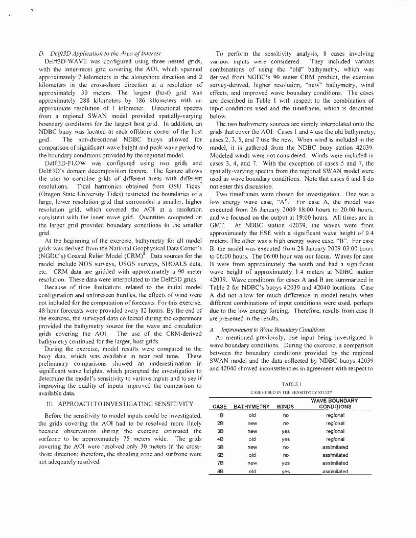
conditions. During the demonstration, offshore wave conditions measured at National Data Buoy Center's (NDBC's) station 42040 showed significant wave heights ranging from 0.5 meters to nearly 2 meters and peak wave periods of 3-8 seconds (Fig. 1).

A. Bathymetry Collection An integral part of any littoral model is the bathymetry.

Wave breaking and nearshore circulation patterns are known to be dependent on depth. During the training exercise, single and multi-beam acoustic survey techniques were employed by The Naval Oceanographic Office's (NAVO's) Fleet Survey Team to collect bathymetric data in the AOI. Single beam surveys were collected from a jet-ski platform. The surveys covered the alongshore extent of the AOI and from the coastline out 700 meters, to a depth of approximately 18 meters. The alongshore line spacing was 25 meters. The multi-beam survey was collected from a boat with a sounding resolution of less than 1 meter. It, too, covered the alongshore extent of the AOI. In the cross-shore direction, it overlapped the offshore 100 meters of the single beam survey and extended out to the offshore boundary of the AOI, roughly 2 kilometers from shore. The single and multi-beam surveys were merged. B. Wave Data

Three types of directional wave buoys were deployed as part of the training exercise. The first, developed at Scripps Institute of Oceanography, is a mini buoy with a diameter of only about 0.2 meters. Although it was originally designed to be a free-floating buoy, preliminary tests were performed, and it was determined that the buoy could perform as a moored platform. The mini buoy will be referred to as Buoy 1 from here forward; it was deployed closest to shore at a depth of approximately 5 meters. Depths given in this section relate to the surveyed bathymetry. Buoy 1 collected data from 27-29 January 2009. Further offshore, but still along the 5 meter

'LM^ 01/27 01/28 01/29 01/30

Time 2009 (mm/dd. GMT)

Figure 1. Comparison of offshore (a) wind speed (meters/second), (b) significant wave height (meters), and (c) peak wave period (seconds) as a

function of time at the NDBC Station 42040. Buoy measurements are represented by the blue line. Model boundary conditions are represented by red x's. The left vertical line represents case A, and the black vertical line to

the right represents case B.

depth contour, a Triaxys buoy was deployed. It will be referred to as Buoy 2. With a diameter of 0.6 meters and a weight of less than 100 kg, it is 2-man deployable. Buoy 2 collected data from 27-31 January 2009, but only significant wave heights will be addressed with respect to Buoy 2. The final wave buoy, referred to as Buoy 3, is a wave sentry buoy developed by QuinetiQ North America. Like Buoy 1, it is in a research and development stage. It is a discus buoy with a diameter of 0.75 meters and is also 2-man deployable. Buoy 3 collected data from 27 January - 5 February 2009. Although some of the buoys remain under development, we consider the data to be truth because the measurements are consistent despite being collected by various platforms. Buoy locations are shown in Fig. 2 with respect to a historical bathymetry referred to as Coastal Relief Model derived; it will be discussed in section D. C. DelftiD in General

The training exercise was an opportunity to test and further develop techniques used to apply Delft3D in an automated, operational fashion. To determine wave conditions, the Simulating Waves Nearshore (SWAN) model is used3'4; it is the wave module of Delft3D (Delft3D-WAVE). SWAN is a spectral wave model that predicts the propagation and transformation of waves and can be used at coarser, regional scales or at higher resolution in littoral environments. The flow module of Delft3D (DelfOD-FLOW) determines the circulation patterns based on the wave averaged Navier-Stokes equations under the shallow water and Boussinesq assumptions5'6. The wave and circulation models are coupled in Delft3D allowing for wave-current interactions and resulting in tidally- and wave-driven currents. Although Delft3D is a 3 dimensional model, our exercise application is in 2 dimensions.

5 14 5 15 5 16 5 17 5

Figure 2. Depths in the area of interest given the old bathymetry. Horizontal and vertical axes represent UTM Eastings (m) and Northings (m), respectively.

The black box shows the region that will be discussed in the results section. Buoy locations are given by three smaller, white shapes—Buoy I: square;

Buoy2: circle; Buoy 3: triangle.

D. Delft3D Application to the Area of Interest Delft3D-WAVE was configured using three nested grids,

with the inner-most grid covering the AOI, which spanned approximately 7 kilometers in the alongshore direction and 2 kilometers in the cross-shore direction at a resolution of approximately 30 meters. The largest (host) grid was approximately 288 kilometers by 186 kilometers with an approximate resolution of 1 kilometer. Directional spectra from a regional SWAN model provided spatially-varying boundary conditions for the largest host grid. In addition, an NDBC buoy was located at each offshore corner of the host grid. The non-directional NDBC buoys allowed for comparison of significant wave height and peak wave period to the boundary conditions provided by the regional model.

Delft3D-FLOW was configured using two grids and DelfOD's domain decomposition feature. The feature allows the user to combine grids of different areas with different resolutions. Tidal harmonics obtained from OSU Tides7

(Oregon State University Tides) restricted the boundaries of a large, lower resolution grid that surrounded a smaller, higher resolution grid, which covered the AOI at a resolution consistent with the inner wave grid. Quantities computed on the larger grid provided boundary conditions to the smaller grid.

At the beginning of the exercise, bathymetry for all model grids was derived from the National Geophysical Data Center's (NGDC's) Coastal Relief Model (CRM)8. Data sources for the model include NOS surveys, USGS surveys, SHOALS data, etc. CRM data are gridded with approximately a 90 meter resolution. These data were interpolated to the Delft3D grids.

Because of time limitations related to the initial model configuration and unforeseen hurdles, the effects of wind were not included for the computation of forecasts. For this exercise, 48-hour forecasts were provided every 12 hours. By the end of the exercise, the surveyed data collected during the experiment provided the bathymetry source for the wave and circulation grids covering the AOI. The use of the CRM-derived bathymetry continued for the larger, host grids.

During the exercise, model results were compared to the buoy data, which was available in near real time. These preliminary comparisons showed an underestimation in significant wave heights, which prompted the investigation to determine the model's sensitivity to various inputs and to see if improving the quality of inputs improved the comparison to available data.

III. APPROACH TO INVESTIGATING SENSITIVITY

Before the sensitivity to model inputs could be investigated, the grids covering the AOI had to be resolved more finely because observations during the exercise estimated the surfzone to be approximately 75 meters wide. The grids covering the AOI were resolved only 30 meters in the cross- shore direction; therefore, the shoaling zone and surfzone were not adequately resolved.

To perform the sensitivity analysis, 8 cases involving various inputs were considered. They included various combinations of using the "old" bathymetry, which was derived from NGDC's 90 meter CRM product, the exercise survey-derived, higher resolution, "new" bathymetry, wind effects, and improved wave boundary conditions. The cases are described in Table 1 with respect to the combination of input conditions used and the timeframe, which is described below.

The two bathymetry sources are simply interpolated onto the grids that cover the AOI. Cases 1 and 4 use the old bathymetry; cases 2, 3, 5, and 7 use the new. When wind is included in the model, it is gathered from the NDBC buoy station 42039. Modeled winds were not considered. Winds were included in cases 3, 4, and 7. With the exception of cases 5 and 7, the spatially-varying spectra from the regional SWAN model were used as wave boundary conditions. Note that cases 6 and 8 do not enter this discussion.

Two timeframes were chosen for investigation. One was a low energy wave case, "A". For case A, the model was executed from 26 January 2009 18:00 hours to 20:00 hours, and we focused on the output at 19:00 hours. All times are in GMT. At NDBC station 42039, the waves were from approximately the ESE with a significant wave height of 0.4 meters. The other was a high energy wave case, "B". For case B, the model was executed from 28 January 2009 03:00 hours to 06:00 hours. The 06:00 hour was our focus. Waves for case B were from approximately the south and had a significant wave height of approximately 1.4 meters at NDBC station 42039. Wave conditions for cases A and B are summarized in Table 2 for NDBC's buoys 42039 and 42040 locations. Case A did not allow for much difference in model results when different combinations of input conditions were used, perhaps due to the low energy forcing. Therefore, results from case B are presented in the results.

A. Improvement to Wave Boundary Conditions As mentioned previously, one input being investigated is

wave boundary conditions. During the exercise, a comparison between the boundary conditions provided by the regional SWAN model and the data collected by NDBC buoys 42039 and 42040 showed inconsistencies in agreement with respect to

TABLE I

CASES USED IN THE SENSITIVITY STUDY

WAVE BOUNDARY CASE BATHYMETRY WINDS CONDITIONS

1B old no regional

2B new no regional

3B new yes regional

4B old yes regional

5B new no assimilated

6B old no assimilated

7B new yes assimilated

8B old yes assimilated

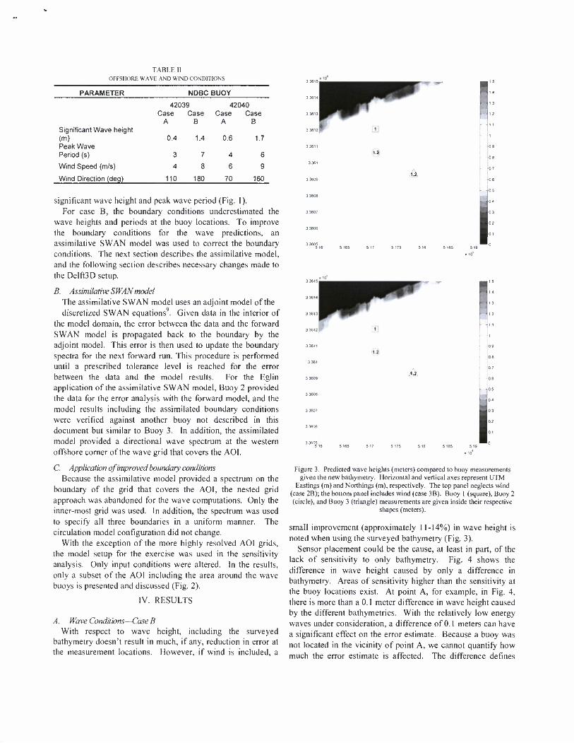
TABLE II OFFSHORE WAVE AND WIND CONDITIONS

PARAMETER NDBC BUOY

42039 42040 Case Case Case Case

A B A B Significant Wave height (m) 0.4 1.4 0.6 1.7 Peak Wave Period (s) 3 7 4 6

Wind Speed (m/s) 4 8 6 9

Wind Direction (deg) 110 180 70 160

significant wave height and peak wave period (Fig. 1). For case B, the boundary conditions underestimated the

wave heights and periods at the buoy locations. To improve the boundary conditions for the wave predictions, an assimilative SWAN model was used to correct the boundary conditions. The next section describes the assimilative model, and the following section describes necessary changes made to the DelfOD setup.

B. Assimilative SWAN model The assimilative SWAN model uses an adjoint model of the discretized SWAN equations9. Given data in the interior of

the model domain, the error between the data and the forward SWAN model is propagated back to the boundary by the adjoint model. This error is then used to update the boundary spectra for the next forward run. This procedure is performed until a prescribed tolerance level is reached for the error between the data and the model results. For the Eglin application of the assimilative SWAN model, Buoy 2 provided the data for the error analysis with the forward model, and the model results including the assimilated boundary conditions were verified against another buoy not described in this document but similar to Buoy 3. In addition, the assimilated model provided a directional wave spectrum at the western offshore corner of the wave grid that covers the AOI.

C. Application of improved boundary conditions Because the assimilative model provided a spectrum on the

boundary of the grid that covers the AOI, the nested grid approach was abandoned for the wave computations. Only the inner-most grid was used. In addition, the spectrum was used to specify all three boundaries in a uniform manner. The circulation model configuration did not change.

With the exception of the more highly resolved AOI grids, the model setup for the exercise was used in the sensitivity analysis. Only input conditions were altered. In the results, only a subset of the AOI including the area around the wave buoys is presented and discussed (Fig. 2).

IV. RESULTS

A. Wave Conditions—Case B With respect to wave height, including the surveyed

bathymetry doesn't result in much, if any, reduction in error at the measurement locations. However, if wind is included, a

„

5 17 5 175 5t

I ,:,

• Jo

5 17 5 175 5 18

Figure 3. Predicted wave heights (meters) compared to buoy measurements given the new bathymetry. Horizontal and vertical axes represent UTM

Eastings (m) and Northings (m), respectively. The top panel neglects wind (case 2B); the bottom panel includes wind (case 3B). Buoy 1 (square), Buoy 2 (circle), and Buoy 3 (triangle) measurements are given inside their respective

shapes (meters).

small improvement (approximately 11-14%) in wave height is noted when using the surveyed bathymetry (Fig. 3).

Sensor placement could be the cause, at least in part, of the lack of sensitivity to only bathymetry. Fig. 4 shows the difference in wave height caused by only a difference in bathymetry. Areas of sensitivity higher than the sensitivity at the buoy locations exist. At point A, for example, in Fig. 4, there is more than a 0.1 meter difference in wave height caused by the different bathymetries. With the relatively low energy waves under consideration, a difference of 0.1 meters can have a significant effect on the error estimate. Because a buoy was not located in the vicinity of point A, we cannot quantify how much the error estimate is affected. The difference defines

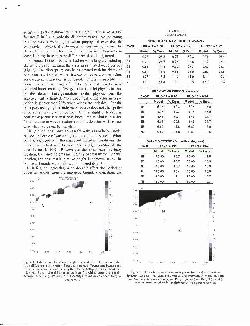
sensitivity to the bathymetry in this region. The same is true for area B in Fig. 4, only the difference is negative indicating that the waves were higher when propagated over the old bathymetry. Note that differences in coastline as defined by the different bathymetries cause the extreme differences in wave heights; these extreme differences should be ignored.

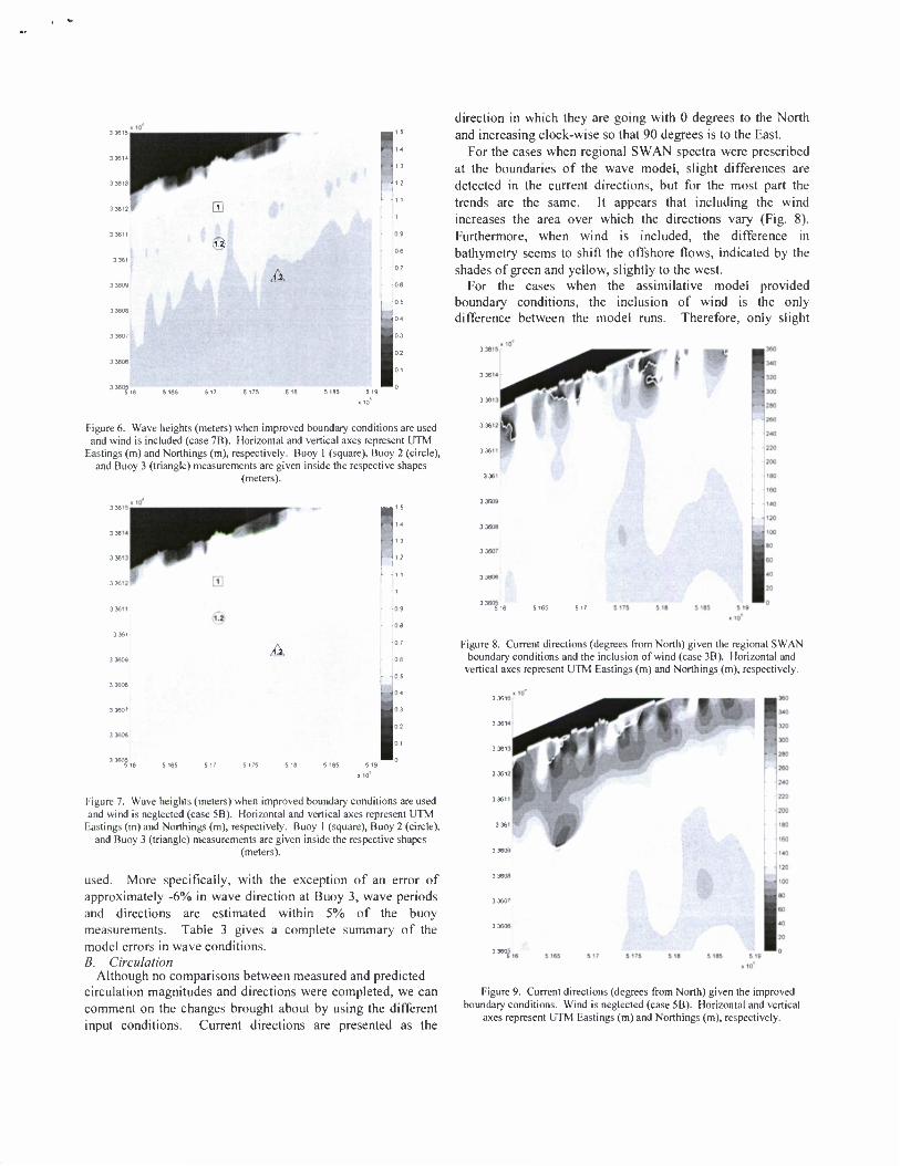
In contrast to the effect wind had on wave heights, including the wind greatly increases the error in estimated wave periods (Fig. 5). The discrepancy can be associated with instability of nonlinear quadruplet wave interaction computations when wave-current interaction is activated. Similar instability has been observed by Rogers10. The presented results were obtained based on using first-generation model physics instead of the default third-generation model physics, but the improvement is limited. More specifically, the error in wave period is greater than 20% when winds are included. For the most part, changing the bathymetry source does not change the error in estimating wave period. Only a slight difference in peak wave period is seen at only Buoy 1 when wind is included. No difference in wave direction results is detected with respect to winds or surveyed bathymetry.

Using directional wave spectra from the assimilation model reduces the error of wave height, period, and direction. When wind is included with the improved boundary conditions, the model agrees best with Buoys 2 and 3 (Fig. 6) reducing, the error by nearly 20%. However, at the most nearshore buoy location, the wave heights are actually overestimated. At this location, the best result in wave height is achieved using the improved boundary conditions and no wind (Fig. 7).

Including or neglecting wind doesn't affect the period or direction results when the improved boundary conditions are

TABLE 111 PERCENT ERRORS

Of I"

SIGNIFICANT WAVE HEIGHT (meters)

CASE BUOY1 =1.00 BUOY 2 = 1.23 BUOY 3 = 1.22

Model % Error Model % Error Model % Error

1B 0.73 27.5 0.74 39.3 0.78 36.4

2B 0.71 28.7 0.75 38.8 0.77 37.1

3B 0.85 14.8 0.89 27.7 0.92 24.3

4B 084 16.5 0.88 28.5 0.92 24.5

5B 1.08 -7.8 1.10 11.9 1.11 10.3

7B 1.13 -11.4 1.15 6.8 1.16 5.3

PEAK WAVE PERIOD (seconds)

CASE BUOY1 = 6.40 BUOY 3 = 6.74

Model % Error Model % Error

1B 5.74 10.3 5.74 14.8

2B 5.74 10.3 5.74 14.8

3B 4.47 30.1 4.47 33.7

4B 5.07 20.8 4.47 33.7

5B 6.50 -1.6 6.50 36

7B 6.50 -1.6 6.50 3.6

WAVE DIRECTIONS (nautical degrees)

CASE BUOY1 = 191 BUOY 3 = 184

Model % Error Model % Error

1B 165.00 15.7 155.00 18.6

2B 165.00 15.7 155.00 18.6

3B 165.00 15.7 155.00 18.6

4B 165.00 15.7 155.00 18.6

5B 185.00 3.1 195.00 -5.7

7B 185.00 3.1 195.00 -5.7

.

I 5 175 5 18 5 185 5 19

Figure 4. A difference plot of wave heights (meters). The difference is related to the difference in bathymetry. Note that extreme differences are because of a difference in coastline as defined by the different bathymetries and should be ignored. Buoy 1, 2, and 3 locations are identified with a square, circle, and

triangle, respectively. Points A and B identify areas of increased sensitivity to bathymetry.

* T

' 6.4 1

(

«:,

5 18 5 165 (

Figure 5. Shows the errors in peak wave period (seconds) when wind is included (case 3B). Horizontal and vertical axes represent UTM Eastings (m)

and Northings (m), respectively, and Buoy I (square) and Buoy 3 (triangle) measurements are given inside their respective shapes (seconds).

3 3612 E

33611

© .1 361

3 3609 A

3 3608

3 3607

3 3606

3 3605 6 5 165 5 17 5 175 5 18 5 185 5

Figure 6. Wave heights (meters) when improved boundary conditions are used and wind is included (case 7B). Horizontal and vertical axes represent UTM

Eastings (m) and Northings (m), respectively. Buoy 1 (square), Buoy 2 (circle), and Buoy 3 (triangle) measurements are given inside the respective shapes

(meters).

• l3

A

2

- 1 1

-

direction in which they are going with 0 degrees to the North and increasing clock-wise so that 90 degrees is to the East.

For the cases when regional SWAN spectra were prescribed at the boundaries of the wave model, slight differences are detected in the current directions, but for the most part the trends are the same. It appears that including the wind increases the area over which the directions vary (Fig. 8). Furthermore, when wind is included, the difference in bathymetry seems to shift the offshore flows, indicated by the shades of green and yellow, slightly to the west.

For the cases when the assimilative model provided boundary conditions, the inclusion of wind is the only difference between the model runs. Therefore, only slight

5 165 5 17

Figure 8. Current directions (degrees from North) given the regional SWAN boundary conditions and the inclusion of wind (case 3B). Horizontal and

vertical axes represent UTM Eastings (m) and Northings (m), respectively.

5 16 5 165 517 5 175 5 18 5 185 5 19

• io'

Figure 7. Wave heights (meters) when improved boundary conditions are used and wind is neglected (case 5B). Horizontal and vertical axes represent UTM

Eastings (m) and Northings (m), respectively. Buoy 1 (square). Buoy 2 (circle), and Buoy 3 (triangle) measurements are given inside the respective shapes

(meters).

used. More specifically, with the exception of an error of approximately -6% in wave direction at Buoy 3, wave periods and directions are estimated within 5% of the buoy measurements. Table 3 gives a complete summary of the model errors in wave conditions. B. Circulation

Although no comparisons between measured and predicted circulation magnitudes and directions were completed, we can comment on the changes brought about by using the different input conditions. Current directions are presented as the

Figure 9. Current directions (degrees from North) given the improved boundary conditions. Wind is neglected (case 5B). Horizontal and vertical

axes represent UTM Eastings (m) and Northings (m), respectively.

differences are noted in the current directions. The trends in these currents are very different than the trends in the cases discussed in the previous paragraph. Here the variability is more cross-shore than long-shore (Fig. 9). Rather than long shore flow to the west in deeper water with alternating areas of onshore and offshore flow in the very nearshore, here we see long shore flow to the west in deeper water and long shore flow to the east in the nearshore. The two areas are separated by a region of offshore currents. In the very nearshore, there are a couple of small areas of onshore flow.

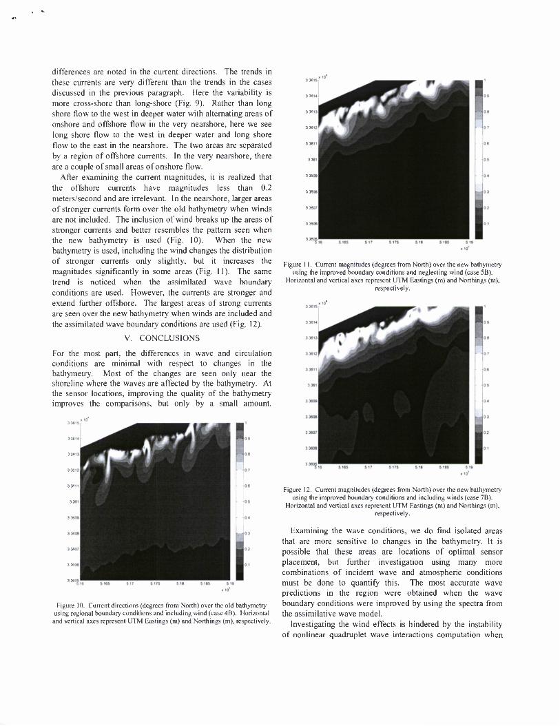
After examining the current magnitudes, it is realized that the offshore currents have magnitudes less than 0.2 meters/second and are irrelevant. In the nearshore, larger areas of stronger currents form over the old bathymetry when winds are not included. The inclusion of wind breaks up the areas of stronger currents and better resembles the pattern seen when the new bathymetry is used (Fig. 10). When the new bathymetry is used, including the wind changes the distribution of stronger currents only slightly, but it increases the magnitudes significantly in some areas (Fig. 11). The same trend is noticed when the assimilated wave boundary conditions are used. However, the currents are stronger and extend further offshore. The largest areas of strong currents are seen over the new bathymetry when winds are included and the assimilated wave boundary conditions are used (Fig. 12).

V. CONCLUSIONS

For the most part, the differences in wave and circulation conditions are minimal with respect to changes in the bathymetry. Most of the changes are seen only near the shoreline where the waves are affected by the bathymetry. At the sensor locations, improving the quality of the bathymetry improves the comparisons, but only by a small amount.

Figure 11. Current magnitudes (degrees from North) over the new bathymetry using the improved boundary conditions and neglecting wind (case 5B).

Horizontal and vertical axes represent UTM Eastings (m) and Northings (m), respectively.

Figure 10. Current directions (degrees from North) over the old bathymetry using regional boundary conditions and including wind (case 4B). Horizontal

and vertical axes represent UTM Eastings (m) and Northings (m), respectively.

Figure 12. Current magnitudes (degrees from North) over the new bathymetry using the improved boundary conditions and including winds (case 7B).

Horizontal and vertical axes represent UTM Eastings (m) and Northings (m), respectively.

Examining the wave conditions, we do find isolated areas that are more sensitive to changes in the bathymetry. It is possible that these areas are locations of optimal sensor placement, but further investigation using many more combinations of incident wave and atmospheric conditions must be done to quantify this. The most accurate wave predictions in the region were obtained when the wave boundary conditions were improved by using the spectra from the assimilative wave model.

Investigating the wind effects is hindered by the instability of nonlinear quadruplet wave interactions computation when

wave-current interaction is activated. Switching to first generation wave option improves the results only slightly. More detailed study using different quadruplet options in SWAN is underway.

Using the improved boundary conditions caused large changes in current magnitudes and directions. Because current data quality control was not completed at the time of manuscript preparation, current measurements were not included in the discussion, and we cannot say which combinations of input conditions most accurately predicted the circulation patterns. More effort is required.

ACKNOWLEDGMENT

The authors thank the Fleet Survey Team, Naval Oceanography Special Warfare Center, and David Lalejini (NRL) for support during the exercise; Eric Terrell (Scripps Institute of Oceanography), Richard Smith (QinetiQ North America), and Gretchen Dawson (NRL) for assistance with the buoys; and Alex Puffer (NRL) for general assistance.

REFERENCES

[ 1 ] Y. L. Hsu, R. R. Mettlach, and M. D. Marshall, "Validation test report for the Navy Standard Surf Model," NRL/FR/73 22-02-10008, Naval Research Laboratory, Stennis Space Center, MS, 2002.

[2] J. D. Dykes, Y. L. Hsu, J. M. Kaihatu, and R. A. Allard, "Development of a Methodology and Software for Operational Delft3D Applications," NRL/MR/7320—05-8832, Naval Research Laboratory, Stennis Space Center, MS, January 2005.

[3] N. Booij, R. C. Ris, and L. H. Holthuijsen, ""A third generation wave model for coastal region: 1. model description and validation," J. Geophys. Res., vol. 104(c4), pp. 7649-7666, 1999.

[4] R. C. Ris, L. H. Holthuijsen, and N. Booij, "A third generation wave model for coastal regions: 2. verification," J. Geophys. Res., vol. 104(c4), pp. 7667-7681, 1999.

[5] G. S. Stelling, "A non-hydrostatic flow model in cartesian coordinates: technical note," Z0901-IO, WL | Delft Hydraulics, The Netherlands, January 1996.

[6] G. R. Lesser, J. A. Roelvink, J. A. T. M van Kester, and G. S. Stelling, "Development and validation of a three-dimensional morphological model," Coastal Engineering, vol. 51, pp. 883-915, 2004.

[7] F. D. Egbert and S. Y. Erofeeva, "Efficient inverse modeling of barotropic ocean tides", J. Atmos. Oceanic Technol., vol. 19, pp. 183-204, 2003.

[8] D. L. Divins and D. Metzger, NGDC Coastal Relief Model, December 2008, http://www.ngdc.noaa.gov/mgg/coastal/coastal.html

[9] Walker, D. T., "Assimilation of SAR Imagery in a Nearshore Spectral Wave Model," GDA1S Report No. 200236, March 2006.

[10] W. R. Rogers, personal communication, August 2009.