validation of the waas mops integrity equation

Validation of the WAAS MOPSIntegrity Equation

Todd Walter, Andrew Hansen, and Per EngeStanford University

ABSTRACT

There has been widespread growth in the number ofdifferential augmentation systems for GPS underdevelopment or in operation. Such systems are beingdeveloped by both civil authorities and commercialinterests. These systems serve a variety of users andapplications including precision approach for aviation,where the system provides vertical and horizontalguidance. Precision approach has very strict requirementsfor accuracy, integrity, continuity, and availability, andthese become more stringent as the decision heightdecreases. To date, it appears that the Wide AreaAugmentation System (WAAS) will be able to meet theaccuracy requirements all the way down to a 200 ftdecision height. The primary concern for such a system isthat it always maintain integrity.

The WAAS Minimum Operational Performance Standards(MOPS) specifies how users combine error confidencesfrom the different sources to form a position bound. Theservice provider guarantees that the error at any userlocation is smaller than the respective bound with asufficiently high confidence. This paper describes thevalidation of the integrity equation. Actual data from theNational Satellite Test Bed (NSTB), a prototype forWAAS, is compared side-by-side to simulated data. Thedifference between actual and expected performance isinvestigated in detail. It is shown that compared to thereal data, the assumptions used in the integrity equationare conservative. Integrity is maintained both in thesimulated data and in the live data. The comparison of thetwo data sets provides insights as to the actual probabilitydistribution of the errors in the live data and aboutcorrelations between different error components. Thisknowledge helps to ensure that the full integri tyrequirements are always met. In the future, it may also bepossible to utilize this information to increase theavailability of the system.

INTRODUCTION

Integrity of a system is often extremely difficult to prove.One must demonstrate safe performance in the past and anexpectation of continued safe operation even in the face ofpotentially unknown threats. Past safe performance canbe demonstrated easily, but it may be difficult o rimpossible to gather enough data to meet stringentrequirements at 10-7 or 10-9 levels. In addition, there isthe question of whether all possible fault modes wereadequately tested. In fact it would not be possible toprove the integrity of any system to a true skeptic.

In order to gain confidence in any system, one must beable to predict the performance of the system under bothnominal and faulted operation. For example, if the errorshave a gaussian distribution with certain means andvariances under “fault free” and various faulted modes ofoperation, performance can be predicted if enough data iscollected to determine those values. This system mustalso be robust against general fault modes to ensure safetyin the face of unexpected errors.

The Wide Area Augmentation System (WAAS) [1]protects the users of the service by providing timelyalarms and bounds on the error in the position solution.These bounds, called protection levels, provide a nindication of the quality of service. In order for thesystem to be usable, the protection levels must be belowpredefined thresholds known as alert limits. The mostchallenging aspect of the system is to generate boundswhich are large enough to always protect the user butsmall enough to permit the operation. At the center ofthis challenge is the integrity equation.

INTEGRITY EQUATION

The WAAS MOPS integrity equation is based on theconcept that the actual pseudorange errors can beconservatively bounded at and beyond the 10-7 probability

Mauna Loa

Honolulu

Sitka

Fairbanks

Kotzebue

Bethel

Cold Bay

Stanford

Riverside

PrescottSan Angelo

Denver

Columbus

Arcata

Seattle Great Falls

WinnipegGreen Bay

Gander

BangorOttawa

Atlantic City

Miami

AndersonDayton

Greenwood

Oklahoma City

Grand Forks

Elko

Figure 1. The NSTB network. Each circle representsthe location of a reference station. The master stationsat the FAA Technical Center and Stanford University areshown as stars. [11]

level by a zero mean gaussian [2] [3]. The variance ofthis gaussian is described in the MOPS [4] and is largelybased on information broadcast to the users from thegeostationary satellite (GEO). Another principle of theintegrity equation is that the pseudorange errors areuncorrelated with one another. This is a conservativeassumption for navigation as the actual correlations appearto be negative. That is, they combine to reduce theoverall positioning error rather than increase it. Forexample, errors common to all pseudoranges will affectthe clock, but will not influence the navigation solution.Additionally, positive errors in the ionospheric estimationmay lead to negative errors in the satellite clock andephemeris terms. When these are combined, the two tendto cancel and reduce the overall error.

The integrity equation is based on covariance propagationfrom errors in the pseudorange domain, ∆∆ y , to the errorin the position domain, ∆∆x . This mapping follows fromthe navigation solution [2] and can be expressed as

∆∆ ∆∆ˆ ˆx y= ⋅ ⋅ ⋅ ⋅ ⋅( )G W G G WT T-1

(1)

where G is the observation matrix and W is theweighting matrix for the measurements. The matrix

G W GT⋅ ⋅( )-1

(2)

is the full position estimate covariance matrix which isavailable when the position solution is calculated. Thevariance of the vertical position estimate is given by thethird diagonal element of this covariance matrix,

σV

≡ ⋅ ⋅( )[ ]G W GT -1

3 3(3)

For WAAS, W is a diagonal matrix and the inverse ofthe ith diagonal element is given by the variance for thecorresponding satellite, σ

i

2 , which is defined as [4]

σ σ σ σ σi i flt i UIRE i air i tropo

2 2 2 2 2= + + +, , , ,

(4)

The four variance terms on the right represent theconfidences for the fully degraded [4] [5] [6] clock andephemeris corrections, σ

i flt,

2 , the fully degradedionospheric correction, σ

i UIRE,

2 , the contribution from theairborne receiver, σ

i air,

2 , and the tropospheric modelcorrection, σ

i tropo,

2 .

The Vertical Protection Level (VPL) is given by

VPLWAAS V

≡ ⋅κ σ( )Pr (5)

where κ ( )Pr is a constant defined in the MOPS whichdepends on the tolerable probability of having an errorgreater than this value. For a 10-7 probability,κ ( ) .Pr = 5 33. For example, if the UDREs, GIVEs,airborne receiver variance, and geometry combined tocreate a σ

V of 2 m, then VPL m

WAAS= 10 66. . This

would indicate that the aircraft would only have onechance in ten million of having a navigation error exceed10.66 meters.

NSTB DATA

The NSTB data presented here was generated using theStanford developed master station code [7]. It is anengineering prototype version of the WAAS masterstation code. It uses the stations shown in Figure 1 togenerate differential corrections applicable throughout theUnited States. The differential corrections are put into theformat specified by the WAAS MOPS [4]. Thus all thecorrection data is passed through the 250 bit per secondbandwidth constraint. The system latency is also ineffect. Although we are infrequently granted access to thegeostationary delivery channel, we always apply the samelatency as though we were.

The ability of the integrity equation to protect users hasbeen borne out over time using the NSTB. Tests includenominal fault free operation and faulted modes. Thesefaulted modes include the use of maneuvering GPSsatellites which the Master Control Segment (MCS) haddeclared “unhealthy,” but were monitored and differentiallycorrected anyway [8]. Also included are six second non-

0 5 10 15 20 250

5

10

15

20

25

σ V (

m)

4

3

2

1

0

0MI:0

MI:

epochs: 0

HMI

epochs: 0

HMI

epochs: 0MI

epochs: 0MI

Alarm Epochs: 8359

System Unavailable

Vertical Performance at Cold Bay, AK 0x2E52 (261343 seconds)

Error (m)

Alarm Epochs: 8359

System Unavailable

96.135%IPV Operation96.135%IPV Operation

epochs: 0MI

epochs: 0MI

90.196%CAT I Oper.90.196%CAT I Oper.

VP

L WA

AS (

m)

Num

ber

of P

oint

s pe

r P

ixel

100

101

102

103

Figure 2. Actual vertical performance at Cold Bay.This is a combined 2-D histogram of error and VPLshowing accuracy, integrity, and availability. The errorscaused by PRN 18 can be seen in the CAT I region.

-10 -8 -6 -4 -2 0 2 4 6 8 10

10-5

100

Cold Bay, AK 0x2E52 (259602 epochs)

Pro

b. o

f Occ

urre

nce

Vertical position error (m)

mean = 0.049238 (m)95% < 1.8 (m)

99.9% > 10 (m)

-5 -4 -3 -2 -1 0 1 2 3 4 5

10-5

100

Pro

b. o

f Occ

urre

nce

Vertical Ratio (Error / σ)

mean = 0.0123595% < 1.299.9% < 1.8

0 5 10 15 20 25

10-5

100

mean = 8.3076 (m)95% < 16 (m)99.9% > 25 (m)

Pro

b. o

f Occ

urre

nce

Vertical Protection Level (m)

Figure 3. Actual vertical performance at Cold Bay.These three histograms show the accuracy, integrity, andavailability separately. Cold Bay had the worstavailability of all our reference stations on these days.

0 5 10 15 20 250

5

10

15

20

25

σ V (

m)

4

3

2

1

0

0MI:0

MI:

epochs: 0

HMI

epochs: 0

HMI

epochs: 0MI

epochs: 0MI


Error (m)

epochs: 0MI

epochs: 0MI

VP

L WA

AS (

m)

Num

ber

of P

oint

s pe

r P

ixel

100

101

102

103

Alarm Epochs: 8359

System Unavailable

Alarm Epochs: 8359

System Unavailable



99.9

%

95%

68%

Figure 4. Simulated vertical performance at Cold Bay.The errors are generated independently for each time andsatellite. For reference, the lines of constant expectedprobability are shown.

-10 -8 -6 -4 -2 0 2 4 6 8 10

10-5

100


Pro

b. o

f Occ

urre

nce


mean = 0.0065192 (m)95% < 3.6 (m)99.9% > 10 (m)

-5 -4 -3 -2 -1 0 1 2 3 4 5

10-5

100

Pro

b. o

f Occ

urre

nce


mean = 0.004344395% < 299.9% < 3.3

0 5 10 15 20 25

10-5

100

mean = 8.3076 (m)95% < 16 (m)99.9% > 25 (m)

Pro

b. o

f Occ

urre

nce


Figure 5. Simulated vertical performance at Cold Bay.Each point is independently generated following agaussian distribution. The center histogram shows theclose agreement between the simulated values (bars) andthe theoretical distribution (solid line).

standard code outages [9] and accelerations larger than thespecification in the Standard Positioning Service (SPS)[10]. In addition several days of solar storms have beenrecorded. Despite these events, the integrity equation wascapable of protecting all users investigated.

It is easy to look at a data set after the fact and describe itscharacteristics. It is more difficult to predict futurebehavior, particularly the integrity of the system. Wehave developed tools to help us examine our data andrapidly identify problems. In particular we have differentways of representing the data. Figure 2 shows a resultfrom three days in June of 1998. This figure shows a twodimensional histogram of the vertical navigation data.The error-VPL space is divided into 25 cm by 25 cm bins.

For every position solution the error is determined bycomparing that solution to the pre-surveyed location ofthe antenna along with the VPL. These two values arequantized to within 25 cm values and the appropriate binof the histogram is incremented. The bins whichcontained one or more data points are shown at theirappropriate location in the error-VPL space. Matlabroutines for generating these figures as well as exemplarcode for formatting the data are available at our web site[12].

We commonly refer to these plots as VPL or “triangle”charts. The chart is broken into three main sections: anunavailable region where the VPL is too large to support

the desired navigation procedure, an unsafe region wherethe VPL supports the operation but the error is largeenough to create Hazardously Misleading Information(HMI), and a usable region where both the VPL and theactual error are below the Vertical Alert Limit (VAL) sothe system is usable and safe. However, it should benoted in normal operation mobile users do not have accessto the actual error. They are entirely dependent on theaccuracy of the VPL. The usable and unavailable regionsare further divided. Above the diagonal line in the trianglechart, the VPL is always larger than the actual error whichis the desired outcome. In the lower right hand regionsthe error has exceeded the VPL and provides MisleadingInformation (MI). Operationally, these regions are notnecessarily hazardous. In the unavailable region, theprocedure will not be flown since the VPL exceeds theVAL, while in the usable region the error is small enoughto keep the aircraft within the obstacle clearance region.Despite these operational considerations, from a systemsstandpoint, the master station and/or integrity equationhave failed to protect the navigation solution if the errorbecomes larger than the VPL. Thus all points should beabove the diagonal line. As can be seen in Figure 2, allpoints are above the diagonal, so for these days, at ColdBay, the integrity requirement was met.

The two most stringent applications for WAAS will beCategory I precision approach (CAT I) and the stillevolving instrument approach with vertical guidance(IPV). These operations have VALs of 12 and 20 meters,respectively. Thus we have further subdivided the usableregion by these two values. If the VPL is below 12meters then the system is usable for CAT I. If it is below20 meters the system will support IPV. If the VPL islarger than 20 meters the system is unavailable for thesestringent applications but may still be usable for non-precision approach, terminal, and en route operations.

This data is typical of the performance we see with ourTestbed Master Station (TMS). It was taken at Cold Bay,which was chosen because it had the worst availability ofall of our reference stations. This is helpful because acommon question on the behavior of our system is theperformance when the VPL is large (low availability). Onthese days, CAT I operations could have proceeded morethan 90% of the time and IPV more than 96%. All otherstations had higher availability, most better than 99.9%for both CAT I and IPV. Again, Cold Bay was chosen forillustrative purposes.

Figure 3 is another way of representing the data. Hereinstead of a two-dimensional histogram we have threeseparate one-dimensional distributions. They show, fromtop to bottom, the accuracy, integrity, and availability ofthe system. As with Figure 2 the probabilities are plotted

on a logarithmic scale. The logarithmic scales are used toemphasize the tails of each distribution. We already havegreat confidence in the TMS operation the vast majorityof the time. We are now interested in exceptions. Themiddle histogram is of primary interest. It shows theratio of actual error to the one sigma value in Equation 3.For reference, a gaussian curve is also shown. Thisparabola would be applicable if all the errors weregaussian, zero mean, and independent. As can be seen, theerrors are more tightly distributed than the gaussianreference. All but seven of the 259,602 data points havevalues less than 2.5. These seven points can also be seenin Figure 2 with a corresponding VPL of roughly 8.5meters.

These seven points clearly belong to a differentdistribution and represent the greatest concern. Thesepoints do not follow the same probability distribution asthe bulk of the errors. Upon investigation it wasdetermined that these points were caused by excessivephase noise on a satellite. Our investigation is stillongoing, but the preliminary evidence is that on June25th, 1998 around 5:19 UTC, SVN 18 (also PRN 18)exhibited phase noise some twenty times larger than thenominal value. All 23 of the NSTB receivers that wereable to track this satellite saw identical effects on their L1and L2 carrier phase measurements. These rapidfluctuations caused the clock error to vary more quicklythan the fast corrections could track, leading to errors thatwere several meters in magnitude. Our prototype softwaredoes not currently have a trap for error sources of thistype. All that is required is a simple clock accelerationcheck which both the WAAS and LAAS systems willhave. However, we have not implemented such traps, inpart to determine and characterize the effects of such errors.It should be noted that this error persisted for more than anhour yet only seven points were driven off of the maindistribution and no errors were larger than theircorresponding VPLs. More detail on this anomaly will bepresented at the end of this paper.

SIMULATED DATA

The real NSTB data described above was used to generate adistribution of observation and weighting matrices. Byusing the same lines of sight, UDREs, GIVEs a n dairborne variances, we could create simulated errors foridentical conditions as experienced with real data. The truerange was defined by taking the known antenna locationsand corrected satellite locations. To this true range weadded simulated noise.

Initially we started with independently distributed zeromean gaussian noise. Each measurement is independent

of all others whether for another satellite or for a differenttime. This result is not intended to reflect actualperformance but to simulate the conditions which areassumed by the integrity equation. As will be seen, thissituation is more conservative than the actualperformance. These results are shown in Figures 4 and 5.

One of the most common questions regarding the trianglecharts is why the data points do not fill in the wholeupper left hand triangular region. This pure gaussian dataset points to part of the answer. Here, as can be seen inFigure 5, the errors are truly gaussian in distribution andfill in the tails as expected yet the distribution of errorsdoes not seem to get much larger as the VPL gets worse.The reason behind this phenomenon is that there are fewerpoints sampled at large VPL. When the VPL is between5 and 11 meters, there are greater than 2,000 data pointsper row. The number of data points per row rapidly dropsdown below 300 for VPLs above 15 meters. Thus thereason the tails seem to decrease at higher VPLs is notbecause the higher VPLs are overly conservative, butrather there are fewer data points in this area. More than95% of the data has a VPL below 16 meters. Themaximum likelihood value for a zero mean gaussian iszero, 68% of the points are contained within one sigma,95% within two sigma and 99.9% within 3.29 sigma.For reference, these lines are shown in Figure 4.

The reference probability lines further illustrate why theupper points tend to be nearer to zero than intuitionexpects. These lines all converge at the origin. Sincetheir slopes are greater than the diagonal line, there ismore space between the 99.9% line and the 10-7 line asthe VPL becomes larger. Thus there is a larger regionwith fewer points going into it resulting in a sparselyfilled appearance. In reality, as many points are in theregion as would be expected given the distribution.

The empty appearance in the upper right part of the saferegion is not due to overcautiousness when the VPLbecomes large. We are not discarding availability in theface of uncertainty. Rather, we are undersampling theregion, and as always, the errors are more likely to besmall than they are to be large. The comparativelysmaller number of points we have at these upper VPLs aremost likely to be distributed near zero. Even if the VPLswere uniformly distributed from 5 to 25 meters, the bulkof the data points would still appear to pull away from thediagonal line at the top as a consequence of the increasingseparation of the lines of constant probability (68%, 95%and 99.9%) from the diagonal line. Only if each discreteVPL level had greater than 107 points (an impossiblylarge number for real data and nearly so for simulated)would the distribution of data appear to fill in the wholeof the upper triangular region.

Temporal Correlations

Correlations in the data will also affect the shape of thedistribution. The real NSTB data contains correlationsacross both time and satellite corrections. To betterunderstand the distribution of the correction errors and anycorrelations between them, we studied the pseudorangeerrors from our real time master station. One difficultywith this method is the lack of a precise truth source.Although we know the location of our reference antennasvery accurately, it is difficult to translate this into precisepseudorange errors. Instead we must contend with errorsin the “truth” reference which may be larger than the errorsin the differential corrections. We separated the correctionerrors into two effects: clock and ephemeris correctionerrors and ionospheric correction errors. The errorcontribution from the user receiver is included in the“truth” reference.

Clock and Ephemeris Correction Errors

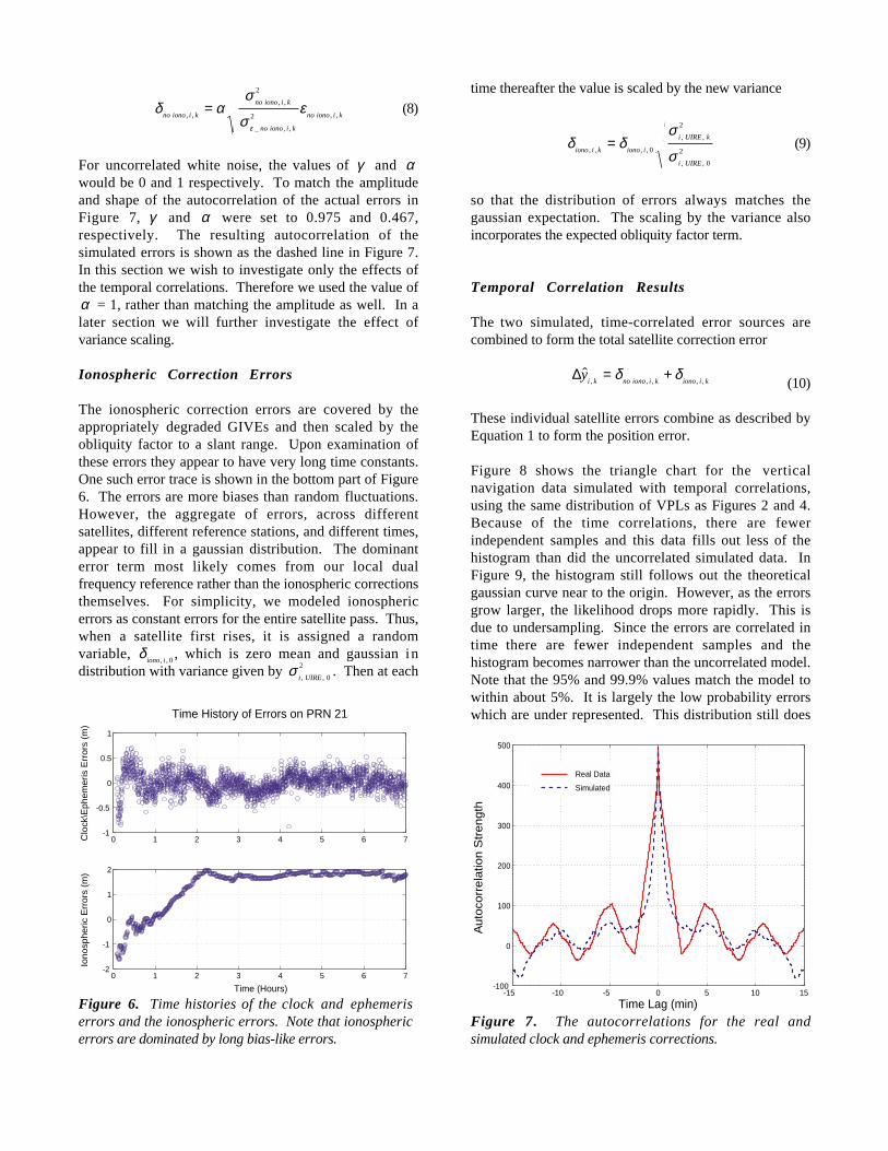
The clock and ephemeris correction errors are covered bythe appropriately degraded UDRE terms in addition to theuser receiver variance. In our case the user is not anairborne receiver, but a static ground receiver at a knownlocation. Even though the reference pseudorangemeasurement can be smoothed using dual frequency carrierphase measurements in post processing, there is still anon-negligible error left. This data for one satellite traceis shown in the top part of Figure 6. The data wasexamined for correlations in time. Common mode errors,as would be expected from the reference clock wereremoved. Figure 7 shows the autocorrelation for the realdata as a solid line. It is clear that the errors are correlatedfor times less than 150 seconds.

In order to simulate this temporal correlation, we used afirst order Gauss-Markov process. The errors weregenerated using

ε γ ε

σ σ γ σε ε

no iono i k no iono i k no iono i k

no iono i k no iono i k no iono i k

w, , , , , ,

_ , , , , _ , ,

= +

= +

−

−

1

2 2 2

1

2(6)

where σno iono i k, ,

2 is given by

σ σ σ σno iono i k flt i k trop i k air i k, , , , , , , ,

2 2 2 2≡ + + (7)

and wno iono i k, ,

is zero mean gaussian variable with variancegiven by σ

no iono i k, ,

2 . The subscript k denotes time. Theactual error applied to the satellite, δ

no iono i k, ,, is scaled to

have the correct variance by

0 1 2 3 4 5 6 7-1

-0.5

0

0.5

1

0 1 2 3 4 5 6 7-2

-1

0

1

2

Time History of Errors on PRN 21

Clo

ck\E

phem

eris

Err

ors

(m)

Iono

sphe

ric

Err

ors

(m)

Time (Hours)

Figure 6. Time histories of the clock and ephemeriserrors and the ionospheric errors. Note that ionosphericerrors are dominated by long bias-like errors.

δ ασ

σε

ε

no iono i k

no iono i k

no iono i k

no iono i k, ,

, ,

_ , ,

, ,=

2

2(8)

For uncorrelated white noise, the values of γ and αwould be 0 and 1 respectively. To match the amplitudeand shape of the autocorrelation of the actual errors inFigure 7, γ and α were set to 0.975 and 0.467,respectively. The resulting autocorrelation of thesimulated errors is shown as the dashed line in Figure 7.In this section we wish to investigate only the effects ofthe temporal correlations. Therefore we used the value ofα = 1, rather than matching the amplitude as well. In alater section we will further investigate the effect ofvariance scaling.

Ionospheric Correction Errors

The ionospheric correction errors are covered by theappropriately degraded GIVEs and then scaled by theobliquity factor to a slant range. Upon examination ofthese errors they appear to have very long time constants.One such error trace is shown in the bottom part of Figure6. The errors are more biases than random fluctuations.However, the aggregate of errors, across differentsatellites, different reference stations, and different times,appear to fill in a gaussian distribution. The dominanterror term most likely comes from our local dualfrequency reference rather than the ionospheric correctionsthemselves. For simplicity, we modeled ionosphericerrors as constant errors for the entire satellite pass. Thus,when a satellite first rises, it is assigned a randomvariable, δ

iono i, , 0, which is zero mean and gaussian in

distribution with variance given by σi UIRE, , 0

2 . Then at each

-15 -10 -5 0 5 10 15-100

0

100

200

300

400

500

Auto

corr

ela

tion S

trength

Time Lag (min)

Real Data

Simulated

Figure 7. The autocorrelations for the real andsimulated clock and ephemeris corrections.

time thereafter the value is scaled by the new variance

δ δσ

σiono i k iono i

i UIRE k

i UIRE

, , , ,

, ,

, ,

=0

2

0

2(9)

so that the distribution of errors always matches thegaussian expectation. The scaling by the variance alsoincorporates the expected obliquity factor term.

Temporal Correlation Results

The two simulated, time-correlated error sources arecombined to form the total satellite correction error

∆ˆ, , , , ,

yi k no iono i k iono i k

= +δ δ(10)

These individual satellite errors combine as described byEquation 1 to form the position error.

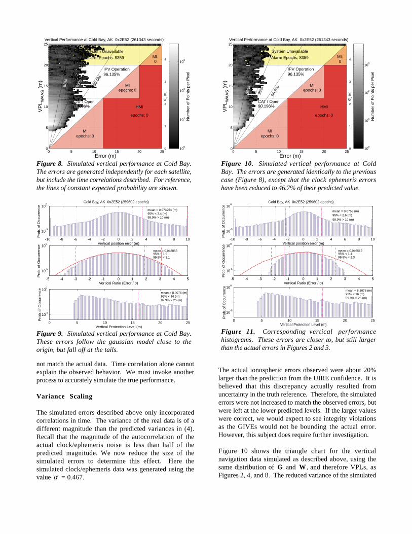
Figure 8 shows the triangle chart for the verticalnavigation data simulated with temporal correlations,using the same distribution of VPLs as Figures 2 and 4.Because of the time correlations, there are fewerindependent samples and this data fills out less of thehistogram than did the uncorrelated simulated data. InFigure 9, the histogram still follows out the theoreticalgaussian curve near to the origin. However, as the errorsgrow larger, the likelihood drops more rapidly. This isdue to undersampling. Since the errors are correlated intime there are fewer independent samples and thehistogram becomes narrower than the uncorrelated model.Note that the 95% and 99.9% values match the model towithin about 5%. It is largely the low probability errorswhich are under represented. This distribution still does

0 5 10 15 20 250

5

10

15

20

25

σ V (

m)

4

3

2

1

0

0MI:0

MI:

epochs: 0

HMI

epochs: 0

HMI

epochs: 0MI

epochs: 0MI


Error (m)

epochs: 0MI

epochs: 0MI

VP

L WA

AS (

m)

Num

ber

of P

oint

s pe

r P

ixel

100

101

102

103

Alarm Epochs: 8359

System Unavailable

Alarm Epochs: 8359

System Unavailable



99.9

%

95%

68%

Figure 8. Simulated vertical performance at Cold Bay.The errors are generated independently for each satellite,but include the time correlations described. For reference,the lines of constant expected probability are shown.

-10 -8 -6 -4 -2 0 2 4 6 8 10

10-5

100


Pro

b. o

f Occ

urre

nce


mean = 0.073254 (m)95% < 3.4 (m)99.9% > 10 (m)

-5 -4 -3 -2 -1 0 1 2 3 4 5

10-5

100

Pro

b. o

f Occ

urre

nce


mean = 0.04885395% < 1.999.9% < 3.1

0 5 10 15 20 25

10-5

100

mean = 8.3076 (m)95% < 16 (m)99.9% > 25 (m)

Pro

b. o

f Occ

urre

nce


Figure 9. Simulated vertical performance at Cold Bay.These errors follow the gaussian model close to theorigin, but fall off at the tails.

not match the actual data. Time correlation alone cannotexplain the observed behavior. We must invoke anotherprocess to accurately simulate the true performance.

Variance Scaling

The simulated errors described above only incorporatedcorrelations in time. The variance of the real data is of adifferent magnitude than the predicted variances in (4).Recall that the magnitude of the autocorrelation of theactual clock/ephemeris noise is less than half of thepredicted magnitude. We now reduce the size of thesimulated errors to determine this effect. Here thesimulated clock/ephemeris data was generated using thevalue α = 0.467.

0 5 10 15 20 250

5

10

15

20

25

σ V (

m)

4

3

2

1

0

0MI:0

MI:

epochs: 0

HMI

epochs: 0

HMI

epochs: 0MI

epochs: 0MI


Error (m)

epochs: 0MI

epochs: 0MI

VP

L WA

AS (

m)

Num

ber

of P

oint

s pe

r P

ixel

100

101

102

103

Alarm Epochs: 8359

System Unavailable

Alarm Epochs: 8359

System Unavailable



99.9

%

95%

68%

Figure 10. Simulated vertical performance at ColdBay. The errors are generated identically to the previouscase (Figure 8), except that the clock ephemeris errorshave been reduced to 46.7% of their predicted value.

-10 -8 -6 -4 -2 0 2 4 6 8 10

10-5

100


Pro

b. o

f Occ

urre

nce


mean = 0.0758 (m)95% < 2.6 (m)99.9% > 10 (m)

-5 -4 -3 -2 -1 0 1 2 3 4 5

10-5

100

Pro

b. o

f Occ

urre

nce


mean = 0.04651295% < 1.499.9% < 2.3

0 5 10 15 20 25

10-5

100

mean = 8.3076 (m)95% < 16 (m)99.9% > 25 (m)

Pro

b. o

f Occ

urre

nce


Figure 11. Corresponding vertical performancehistograms. These errors are closer to, but still largerthan the actual errors in Figures 2 and 3.

The actual ionospheric errors observed were about 20%larger than the prediction from the UIRE confidence. It isbelieved that this discrepancy actually resulted fromuncertainty in the truth reference. Therefore, the simulatederrors were not increased to match the observed errors, butwere left at the lower predicted levels. If the larger valueswere correct, we would expect to see integrity violationsas the GIVEs would not be bounding the actual error.However, this subject does require further investigation.

Figure 10 shows the triangle chart for the verticalnavigation data simulated as described above, using thesame distribution of G and W , and therefore VPLs, asFigures 2, 4, and 8. The reduced variance of the simulated

-40 -30 -20 -10 0 10 20 30 4010

15

20

25

30

-40 -30 -20 -10 0 10 20 30 40-10

0

10

20

30

40

PRN 16: Nominal Operation

PRN 18: Faulted Operation

Time - June 25, 1998 05:19:45 UTC (sec)

Clo

ck E

rror

(m

)C

lock

Err

or (

m)

Calculated Clock ErrorSimulated WAAS MessageExtrapolated Correction

Figure 12. Normal satellite behavior shown up top forPRN 16 and excessive accelerations shown below forPRN 18. Also shown are the simulated effects on theWAAS fast correction messaging. Not shown is thealarm response of the system.

noise decreases the error in the navigation solution. Thetriangle chart for this data looks much more like the actualdata in Figure 2. However, as can be seen in Figure 11,the distribution of errors is still more than 20% larger.The temporal correlations for these simulated data areconservative compared to the actual data. Theclock/ephemeris terms match closely, but we assumedworse correlations for the ionospheric corrections. Also,the magnitudes of the errors either match (for clockephemeris) or are smaller than the real data (forionospheric corrections). Despite this, the resultingsimulated position solution is still worse than the realdata! This discrepancy arises because we have onlyincorporated correlations in time. There are obviouslycorrelations between the different error sources which tendto reduce the overall position error.

SATELLITE ANOMALY

The integrity equation works because the errors are eitheruncorrelated or beneficially correlated. Thus they do nottend to combine in a worst possible fashion. Theanomalous points in the real data shown in Figures 2 and3 reflect a failure mode on a single satellite. SVN 18exhibited large accelerations and jerk in its clock signal.As mentioned, all 23 stations viewing the satelliteobserved identical behavior in their L1 and L2 carrierphases.

Figure 12 shows the time history of clock error asdetermined by our TMS for both PRN 16 and PRN 18.Notice that PRN 16 exhibits the expected behavior forselective availability. In this figure we have also placed asimulated WAAS message. A fast correction message isgenerated every 6 seconds and is based on 18 seconds ofprevious data which is then forward predicted to accountfor a 4 second latency [5]. Each correction is alsodiscretized by 0.125 meters and then used to extrapolatethe simulated WAAS correction shown by the solid line.As can be seen, this process provides a correction for PRN16 accurate to better than a meter. However, for PRN 18,the large accelerations and sudden sign changes combinedwith the message rate and latency result in a very poorcorrection message. Here the errors can be off by as muchas 10 meters.

In the region between -5 and 10 seconds, the clockacceleration changes from greater than 200 mm/s2 to lessthan -150 mm/s2 and back greater than 170 mm/s2.Remember that the Standard Positioning Service (SPS)specification for the magnitude of the clock acceleration isnot to exceed 19 mm/s2 [13]. Thus we have accelerationsgreater than 10 times the specification and rapid changesas well. This is more than the WAAS messaging system

can keep up with. If we had implemented a moresophisticated acceleration trap, as will be in place for theoperational WAAS and LAAS systems, we could haverecognized and flagged this problem before data wastransmitted to the user. As it was, our TMS recognized aproblem and broadcast fast clock corrections more oftenthan every six seconds to mitigate this problem. Thus,within the required six second time to alarm, when oursystem recognized that the user would suffer anunacceptably large error, it sent out an emergencycorrection message (not shown in Figure 12).Operationally there were no ill effects as the VPL alwayscovered the actual error. However, we feel the system canbe made to perform better if we installed the kind of errorhandling that will be present in the operational system.In this case, the seven anomalous points will either berecognized and removed beforehand, or the UDRE will besufficiently increased to account for this unusual satellitebehavior. Again it should be noted that this anomalousbehavior persisted for hours yet only seven points departedfrom the nominal distribution and no points led tointegrity violations.

CONCLUSIONS

This paper has addressed two key assumptions of theintegrity equation: the position errors can be overboundedat the tails by a zero mean gaussian with specifiedvariance, σV, and the errors do not combine in a worst casefashion. The data in Figures 2 and 3 demonstrate that thereal errors are always bounded by the VPL. In addition,the data is more tightly distributed than the reference

gaussian curve. We have seen these effects at everyreference station, over numerous data sets spanning manyyears.

The weighting matrix for the integrity equation i sdiagonal, meaning that any correlations between thesatellites are ignored. Also the variances for the individualerror components for a single satellite are combinedassuming independence (4). We have asserted that this isa conservative assumption because in reality they arecorrelated in such a manner so as to reduce the overallerror. This has been demonstrated via the simulated data.Figures 10 and 11 incorporated conservative assumptionsabout correlations in time and the magnitudes of the errorcomponents yet the resulting distribution is still largerthan the actual one. We did not simulate correlationsbetween the satellites. At a minimum such correlationsdo not appear to inflate the error and all of the evidence todate suggests that they in fact reduce it. This is theexpected outcome from analysis as well, given thatcommon errors affect only the clock, and an error in onepart of a satellite’s correction will tend to create anoffsetting error in another part.

The anomalous points in the real data lead to a weaknessin the Stanford generated UDREs and not in the integrityequation itself. Although the errors were subsequentlycorrected within the six second time to alarm, a nalgorithm exists which could have prevented theirtransmission altogether. It is important to note thatdespite having clock errors on PRN 18 much larger thanwhat is protected by the UDRE, these errors combinedwith other satellites to create a small overall positionerror. Thus, even in a faulted mode, the errors combinedin a beneficial manner.

The real data shows the VPLs to be nearly twice as largeas they need to be. Unfortunately we are already using thelowest possible values for UDRE and have reduced thedegradation parameters as well. However, the observedvariance of the errors appears to be significantly lowerthan the MOPS allows the master station to predict.Unfortunately the broadcast UDREs are also coarselydiscretized and for safety the master station must broadcastthe next larger value. Thus the MOPS forces much ofthis conservatism. However, some of it is a reflection ofconservatism on the part of our master station.

Ideally, as these error sources become better understood wewill be able to reduce the UDREs and GIVEs and hencethe VPLs for the users. This will increase availability atstations such as Cold Bay, our worst station, and increasethe margin of availability and continuity at other stationsalready having high availability.

ACKNOWLEDGMENTS

This work was sponsored by the FAA GPS Product Team(AND-730). We would also like to thank our colleaguesat the Wide Area Differential GPS lab at StanfordUniversity for their many contributions to this work.

REFERENCES

[1] Loh, R., Wullschleger, V., Elrod, B., Lage, M., andHaas, F., “The U.S. Wide-Area Augmentation System(WAAS),” NAVIGATION, Fall 1995.

[2] Walter, T., Enge, P., and Hansen, A., “A ProposedIntegrity Equation for WAAS MOPS,” in proceedings ofION GPS-97, pp. 475-484, Kansas City, MO, September1997.

[3] Walter, T., Enge, P., and Hansen, A., “IntegrityEquations for WAAS MOPS,” in Global PositioningSystem: Papers Published in NAVIGATION Volume VI,to be published 1999.

[4] RTCA Special Committee 159 Working Group 2,“Minimum Operational Performance Standards for GlobalPositioning System / Wide Area Augmentation SystemAirborne Equipment,” RTCA Document Number DO-229A June 1998.

[5] Walter, T., “WAAS MOPS: Practical Examples,” inproceedings of ION National Technical Meeting, SanDiego, CA, Janurary 1999.

[6] Slattery, R., Peck, S., Anagnost, J., and Moon, M.,“Guaranteeing Integrity for all Users of Active Data,” inGlobal Positioning System: Papers Published inNavigation Volume VI to be published 1999.

[7] Enge, P., Walter, T., Pullen, S., Kee, C., Chao,Y.C., Tsai, Y.J., “Wide Area Augmentation of the GlobalPositioning System,” in Proceedings of the IEEE, Vol.,84, No. 8, August 1996.

[8] Tsai, Y. J., “Wide Area Differential Operation of theGlobal Positioning System: Ephemeris and ClockAlgorithms,” Stanford University Ph. D. Dissertation,June 1999.

[9] Cobb, H. S., Lawrence, D., Christie, J., Walter, T.,Chao, Y. C., Powell, J. D. and Parkinson, P., “ObservedGPS Signal Continuity Interruptions,” in Proceedings ofION GPS-95, Palm Springs, CA, September 1995.

[10] Hansen, A., Walter, T., Lawrence, D., and Enge, P.,“GPS Satellite Clock Event of SV#27 and Its Impact onAugmented Navigation Systems,” in proceedings of IONGPS-98, Nashville, TN, September 1998.

[11] Wessel, P. and Smith, W. H. F., “New Version ofthe Generic Mapping Tools Released,” EOS Trans. Amer.Geophys. U., Vol. 76, pp 329, 1995.

[12] http://waas.stanford.edu

[13] Global Positioning System Standard PositioningService Signal Specification, June 1995.

validation of the waas mops integrity equation

Documents